Air Changes for Healthy Indoor Ambiences under Pandemic Conditions and Its Energetic Implications: A Galician Case Study


1
Department of Nautical Science and Marine Engineering, E.T.S.N. y M., University of A Coruña, Paseo de Ronda 51, 15011 A Coruña, Spain
2
Beneficiary of an AXA Research Fund Postdoctoral Grant, Research Leaders Fellowships, AXA SA 25 Avenue Matignon, 75008 Paris, France
3
LEMA, ArGEnCo Department, University of Liège, 4000 Liège, Belgium
*
Author to whom correspondence should be addressed.
Appl. Sci. 2020, 10(20), 7169; https://doi.org/10.3390/app10207169
Submission received: 16 September 2020
/
Revised: 10 October 2020
/
Accepted: 12 October 2020
/
Published: 14 October 2020
(This article belongs to the Special Issue Efficiency and Optimization of Buildings Energy Consumption: Volume II)
Abstract
:Featured Application
An analysis of the optimal ventilation level in naturally ventilated classrooms under COVID-19 pandemic requirements.
Abstract
The present paper aims to show a mathematical understanding of the effect of ventilation rate over building energy consumption. Moreover, as a case study to show this methodology, a proposal was analyzed of modifying the teaching period to reach a maximum increase of air changes in school buildings, to allow adherence to the COVID-19 pandemic requirements in the Galicia region, with lower energy consumption. In this sense, to analyze the energetic implication of this proposal, the building construction was defined, modeled in accordance with the ISO Standard 13790 and implemented in accordance with the Monte Carlo method. Results showed the probability of energy consumption as a Weibull model. Furthermore, a map of different Weibull models in accordance with different ventilation rates was developed. The constants of the Weibull models allow to identify normal distributions of the probability density functions of energy consumption, especially the ones with lower energy consumption. As a consequence, these constants are a better parameter to identify the optimal ventilation rate for each season in search of a healthy indoor ambience, which is of interest for a future design guide. Finally, the main results showed a reduction of energy consumption at a higher ventilation rate in the summer season. As a consequence, the necessity of modifying teachings periods, as an adequate procedure to prevent more COVID infections, is concluded.
1. Introduction
Indoor ambiences are controlled to reach an adequate thermal comfort, ensuring healthy conditions. In this sense, in mild climates with high relative humidity, such as in the Galicia region, there is no need of complex Heating Ventilation and Air Conditioning Systems (HVAC) in most public buildings, such as schools and offices. Most of the time, solely a hot water system fed by a fuel oil boiler is employed during the coldest winter days, with an average relative humidity of 80%. Moreover, the ventilation rate is manually controlled by opening windows in accordance with common sense and the occupant’s perception of indoor air quality. This perception, in accordance with previous research works [1], depends on the time that an occupant stays in that indoor environment, which reaches the lowest perception of air quality after some minutes in that environment. As a consequence, the need for natural ventilation and air renovation arises, most of the times in public buildings, when the level of indoor quality has worsened significantly.
ASHRAE [2] has proposed increasing the ventilation rate due to the COVID-19 pandemic. In this sense, “transmission of COVID-19 through the air is sufficiently likely that airborne exposure to the virus should be controlled. Changes to building operations, including the operation of heating, ventilating, and air-conditioning (HVAC) systems, can reduce airborne exposures” [2]. All these changes must be done in agreement with the ASHRAE Standard 62.1-2019. In particular, some designer guidelines for general schools proposed by the ASHRAE recommend that relative humidity in the winter season must not decrease below 50% due to that it increases the probability of COVID-19 propagation, which is not a problem for the humid region of Galicia. Moreover [3], it recommends installing CO2 sensors at the occupied zone that warn against underventilation and, during the epidemic, to change the default limits to 800 ppm (warning) and 1000 ppm (alarm). Moreover, if mechanical ventilation is not employed, it is proposed to employ HEPA air purifiers. Despite this, an adequate air renovation and dilution of contaminants are required. As a consequence, it is recommended to ensure that the airflow patterns in classrooms are adjusted to minimize occupant exposure to particles [2]. As a consequence, different laminar air movements are required to prevent aerosols, which create a high to spread the COVID-19 through air flow [4]. Moreover, all these comments are in agreement with the World Health Organization (WHO) [5] proposing to increase ventilation when the climate allows.
Finally, energy consumption is one of the most important factors to be considered during the designing of new constructions, and these need to be improved in the existing buildings, as was shown in recent research works [6,7,8,9,10,11]. In this sense, there are a lot of software resources that can be used to estimate building energy consumption during the full year and different standards for building energetic qualification [12,13]. One of the main objectives of the International Energy Agency [14] is to obtain new methodologies for defining better alternatives for preventing energy consumption in buildings; there is currently a knowledge gap in this field. Currently, there is no real understanding of the ventilation in buildings, which reduces the options of improvement proposals. As a consequence, the aim of this work is to analyze the energetic effect of the air changes in buildings and to identify the guide parameters to increase the ventilation rate. In particular, a case study of this procedure in a Galician school building, in accordance with the pandemic requirements, was shown. In this sense, a calculation procedure based on ISO Standard 13790 was developed in accordance with the Monte Carlo method [15,16,17] with the aim to obtain an original result not shown by software resources of building energy rating; additionally, a probabilistic model for energy use was employed in accordance with a Weibull distribution [18,19,20,21,22]. Furthermore, this probabilistic model will be employed to define the expected energy consumption at different ventilation rates and weather conditions and to identify the better options to reach a healthy indoor ambience with lower energy consumption.
2. Materials
2.1. Climatic Data
Climatic data were collected through a sampling process in 50 weather stations located in central and remarkable points in Galicia. These weather stations sample temperature, relative humidity, and wind speed variables with a sampling frequency from about 5 to 10 min [12,23] and an error margin of 0.1 °C, 0.2%, and 0.1 m/s, which can be considered acceptable. Moreover, these weather stations were chosen for the purpose of this study because they ignore buildings and other conditions that could possibly interfere with the data.
2.2. School Buildings
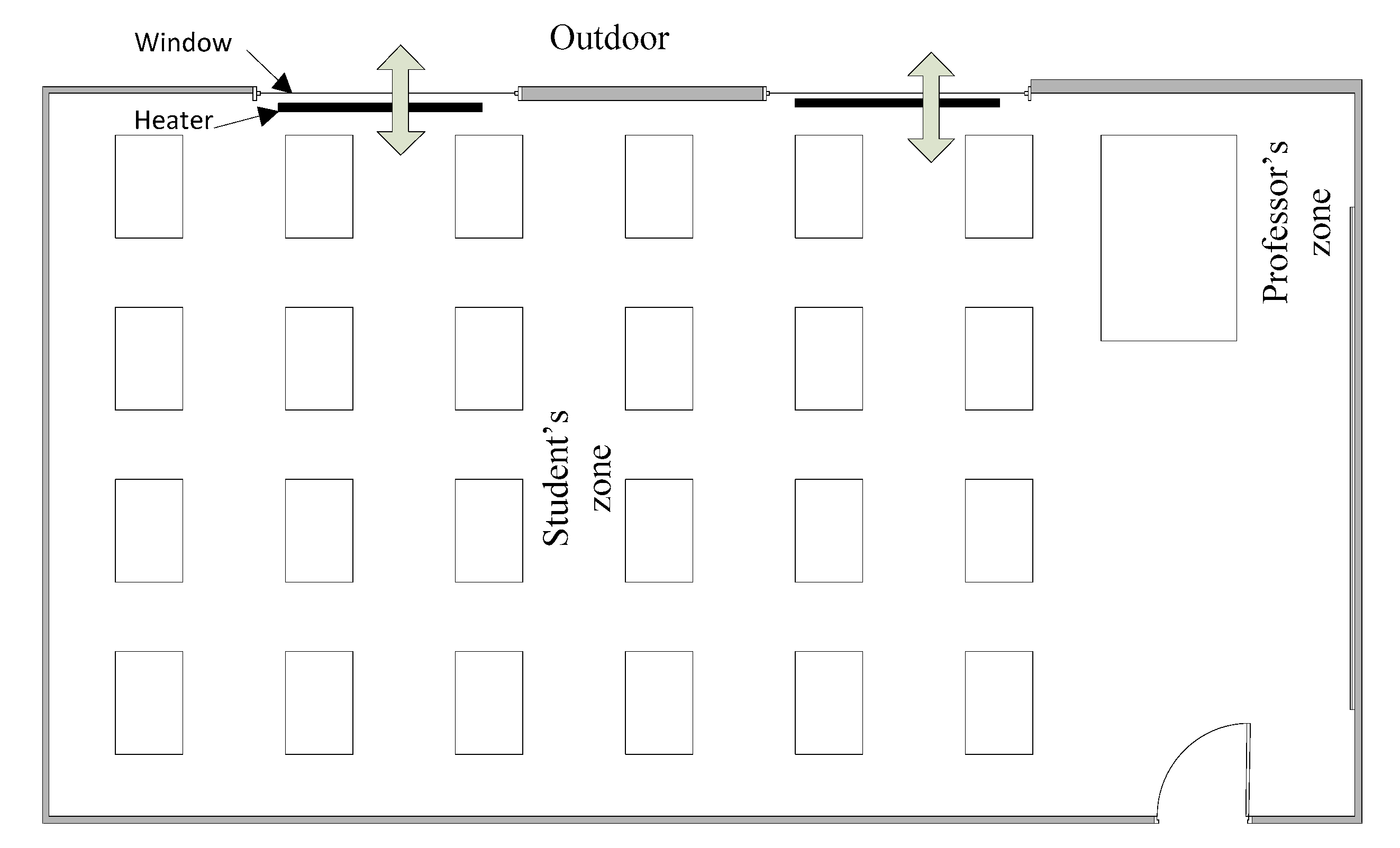
The school building selected for this case study is placed in Galicia, in the northwest of Spain. In this school building, the average classroom occupation level is 25 occupants, with an average floor area of 50 m2, in accordance with the COVID-19 pandemic requirements based on the Galician Ministry recommendations.
The school was built using concrete with walls of two brick layers thick, and an internal air barrier. The floor is in direct contact with the ground, and not insulated. Concurring with earlier research works [24], the internal heat capacity of the building was calculated in accordance with the EN ISO 13790 standard, and the resulting value was found to be 150 kJ/(m2 K). This value corresponds to a medium heavy structure. Finally, the U-value for the windows is 1.8 W/m2K, in accordance with the low emissive and double-glazed windows.
In line with previous research works on thermal inertia, typical wall constructions were defined, and minimum and maximum wall thermal inertia were defined in accordance with the standards. In light of this, values between 150 kJ/(m2 K) and 400 kJ/(m2 K) were selected to be employed in the next simulation processes.
Finally, this classroom has natural ventilation through windows that can be opened manually, reaching an average ventilation level of 0.8 air changes per hour in winter and summer seasons. This value was obtained with the tracer gas decay method, employing SF6 as sampled gas. The geometry of the typical school building is shown in Figure 1, and shows two zones: the professor’s zone and the student’s zone.
2.3. Internal Heat Gains
The proposed values of internal heat gains in the EN ISO 13790 standard can be used if no national data are available. Therefore, the simulations were adapted to the actual situation. The sum of the internal heat gains from occupants, lighting, and devices gives the annual internal heat gains, which are proposed in the standard, as constant values 5.7 W/m2 for school buildings. In our case study, concurring with previous research works [25], the real annual internal heat gain was analyzed and fixed at 44 kWh/m2 year.
2.4. HVAC System Set Point Temperature
The heating system typically employed in Galician classrooms consist of a central heating system consisting of a fuel boiler that heats water at 80 °C and, once mixed with return water, is circulated in different classrooms. In particular, the building objective of this study is heated continuously for about 4 h, which represents part of the working period. In this sense, in accordance with the ISO Standard recommendations for this region, the set point of heating and cooling is 18 °C and 23 °C, respectively, to maintain better thermal comfort while maintaining low energy consumption.
3. Methods
As was commented before, the methodology employed in the present study aims to define the probability density function of energy consumption during the winter and summer seasons in buildings. With this information, different ventilation levels of the classroom in the Galician region will be analyzed to identify the real effects and requirements of a COVID-19 pandemic situation.
Despite the fact that all the methods are explained in this section, an in-depth definition of the Monte Carlo method over ISO 13790, taking as reference some residential building, can be seen in previous work [26]. Moreover, in this previous research, the results obtained with this methodology were validated with respect to the certified energy rating software resources.
3.1. ISO 13790 Standard
This ISO 13790 Standard was developed by the European Committee for Standardization (CEN), in collaboration with the International Organization for Standardization (ISO) to define the calculation methodology of the energy consumption and carbon dioxide emissions in buildings. Despite the fact that ISO employs different levels of calculation complexity, for the present paper, the annual energy use method was employed.
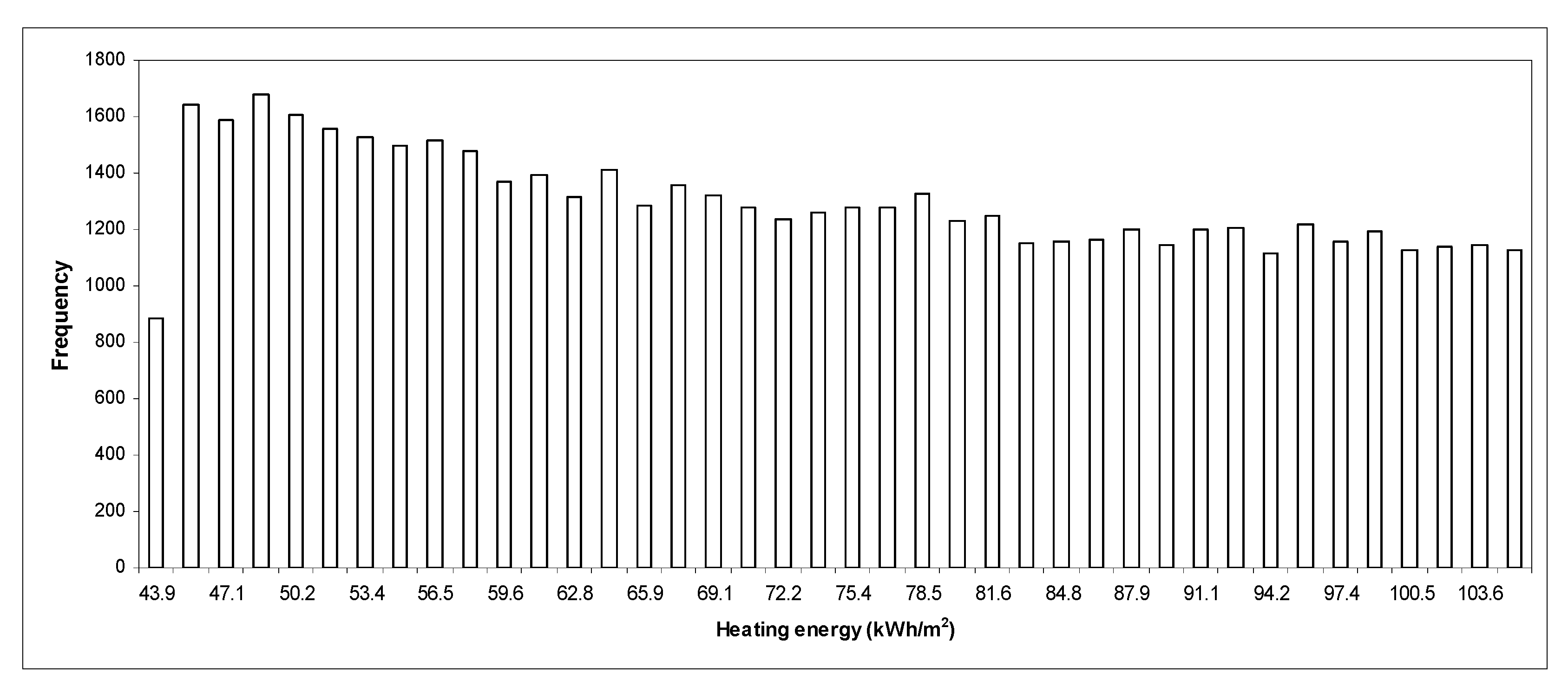
The process begins with a selection of the main variables that must be considered in the building’s energy consumption. In this sense, variables such as indoor air temperature in winter and summer seasons, building thermal inertia, air changes and the number of occupants were selected in accordance with ISO Standard 13790 and adjusted to the values of a real building [27,28,29,30,31,32,33]. From any modification of these values, when the outdoor air temperature is entered in a random way in accordance with the Monte Carlo Method procedure, the probability distribution of the expected energy consumption due to each building modification is obtained. In the base case, the number of air changes was 0.8, thermal inertia was 150 kJ/m2 K, and the number of occupants was 25. At the same time, the average outdoor temperature conditions were defined in accordance with the ISO Standard indications for the region objective of this study. The heating and cooling systems, with set point temperatures of 18 °C and 23 °C, were identified with energy performance indices of 0.7 and 2.55, respectively. Subsequently, once the random input data were entered, the corresponding histograms were developed, as shown in Figure 2, and the probability density function of heating and cooling energy consumption for different air change values was defined, as shown in Figure 3, Figure 4, Figure 5, Figure 6, Figure 7 and Figure 8. Finally, it is of interest to highlight that, as shown in previous works, the effect of thermal inertia does not exist in these kinds of yearly studies about energy consumption.
3.2. Calculation Process: Number of Iterations
The random process was developed in Visual Basic for Applications for each different curve to obtain an adequate determination factor during the curve fitting process. In this sense, the Monte Carlo method predicts the estimation of the total error (ε), which is proportional to the number of iterations, by Equation (1):
where σ is the standard deviation of the random variable and N is the number of iterations.
For instance, in the present case study, the standard deviation of the outdoor temperature was 1.45 °C in the summer and 2.09 °C in the winter season and the minimum number of iterations required for an error less than 2% was calculated. As a consequence, the minimum number of iterations proposed for each season was 166 in winter and 86 in summer season. Due to the fact that the ISO procedure needs few calculations and the curve fitting needs the highest number of values possible, an iterative process was developed with more than 60,000 iterations.
However, after a curve fitting in accordance with more than 60,000 mathematical models, a Weibull density distribution was selected in accordance with the determination factor obtained. The curve fitting process was done with the CFtool of Matlab software. Despite this, the codification was implemented by the authors to develop this task automatically, and to order the obtained curves by its determination factor. Within the 10 more accurate equations obtained, the Weibull model was selected due to its well-known relation with processes that change its probability density function during its life, as it used to be in maintenance models.
As a consequence, this adequate curve fitting could be identified by a determination factor of 0.90 between the simulated data and the values defined by the Weibull model of Equation (2):
where x is the input variable and a0, b0, c0, d0, and e0 are the model constants.
4. Results and Discussion
Once the Monte Carlo Method was applied in the calculation procedure defined by the building Standard ISO 13790, with more than 60,000 runs, the frequency of each different value was defined, as shown in Figure 2.
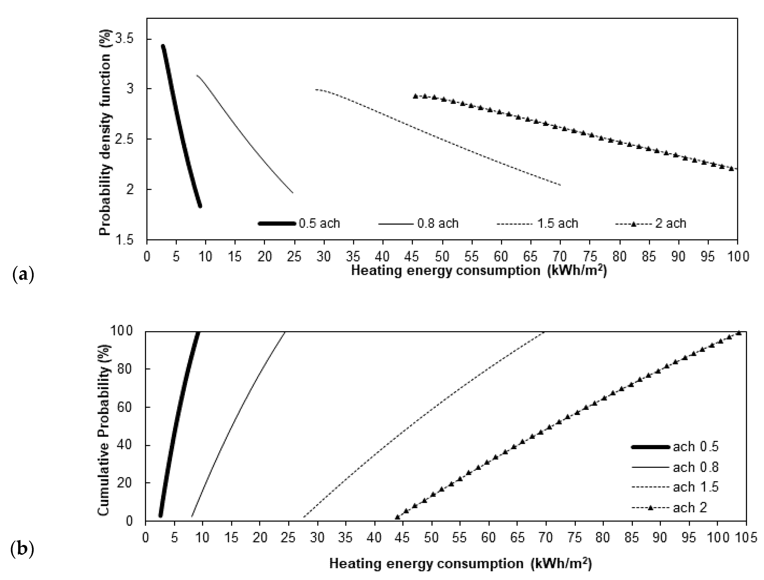
This histogram could be curve fitted for each different study in accordance with the Weibull distribution model of Equation (2) with an adequate determination factor, as can be observed in Figure 3.
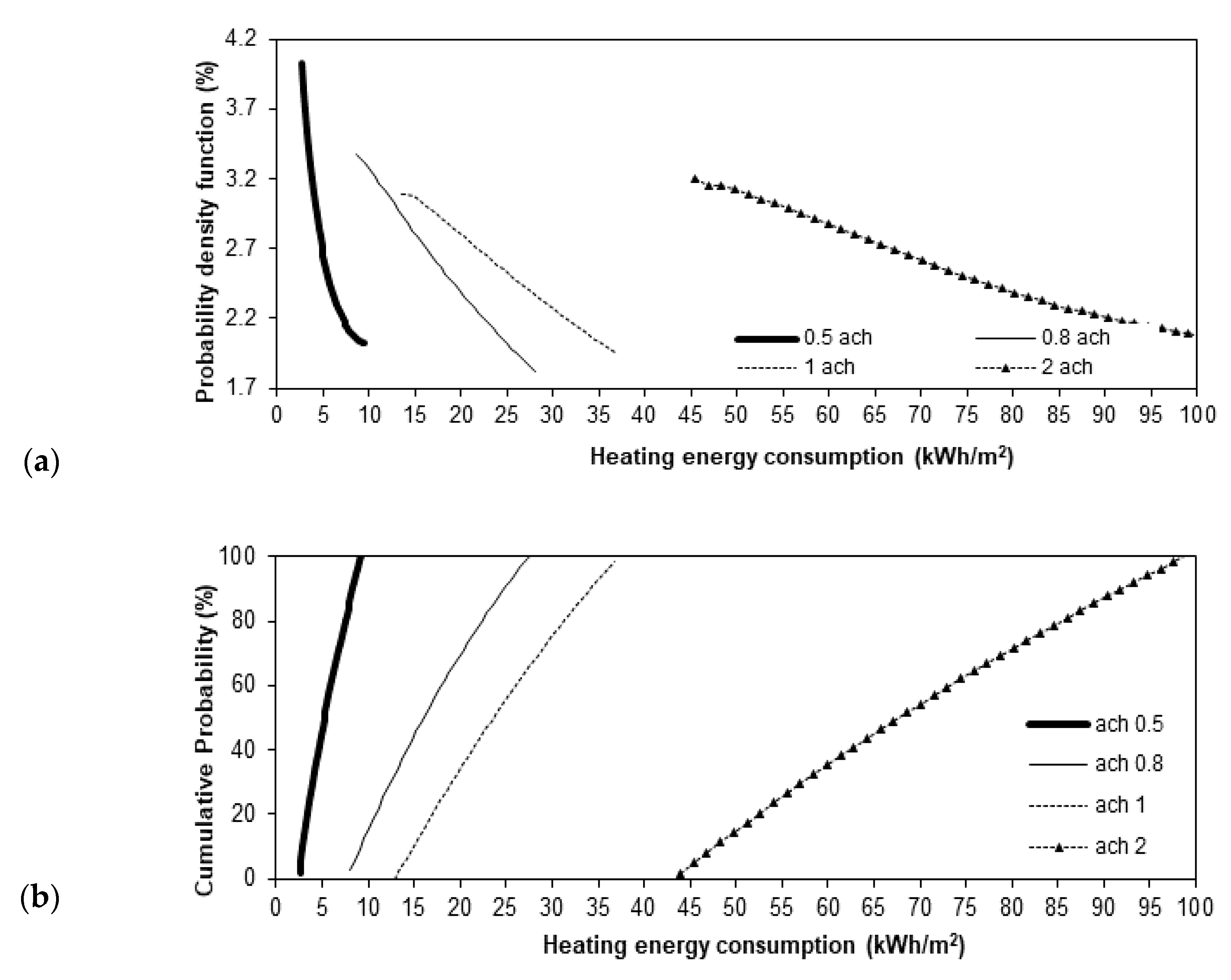
After simulating the actual conditions, based on the values obtained from weather stations in Galicia and ISO 13790 standards indications, and in accordance with the yearly variation of the average temperature in winter and summer season of 0.5 °C and 1 °C [34], the Monte Carlo method was applied again with this temperature increase in the mean outdoor temperature. As a consequence, Figure 4, Figure 5, Figure 6, Figure 7 and Figure 8 were obtained.
As an initial comparative parameter between Weibull models, we can use the value of the model constants shown in Table 1 and Table 2 obtained from a curve fitting process for heating and cooling seasons at different average air temperatures and air changes. At the same time, the point of maximum probability value of each cumulative curve is of real interest, due to that it is the highest energy consumption possible; moreover, the maximum of the probability density function has been analyzed, as it represents the more frequent value of energy consumption.
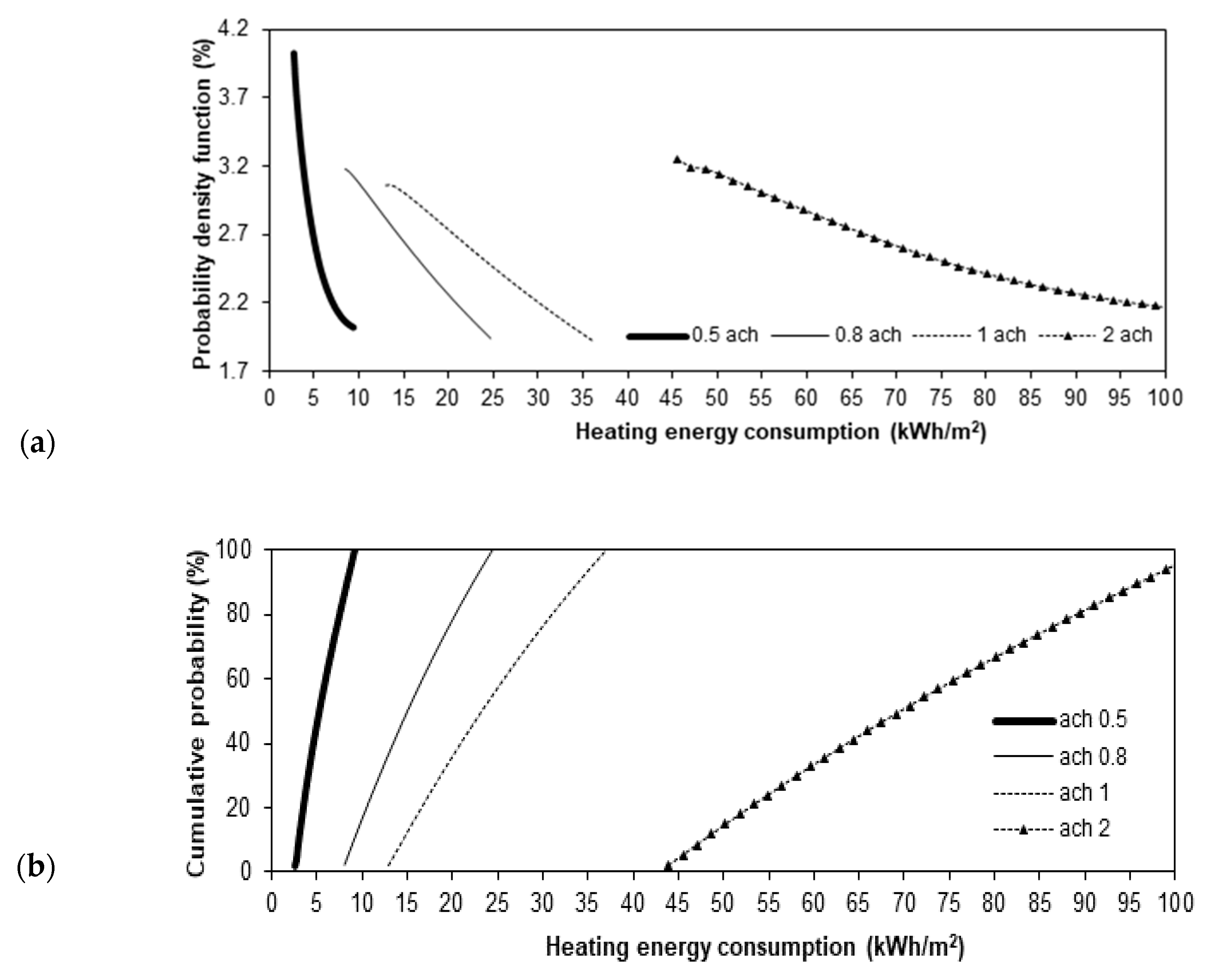
In this sense, in Figure 3a the curve of the probability density function of the heating energy consumption after a 0.5 ach shows a more probable energy consumption of 2.89 kWh/m2 with a frequency of 3.39% of the cases. Despite this, the energy consumption may reach 9.03 kWh/m2, as we can see at the end of this same curve. If we now employ the cumulative curve of Figure 3b and we locate the cut of the 0.5 ach curve with the 100% cumulative probability, it can be concluded that all the energy consumption after a 0.5 ach will be equal to or lower than 9.03 kWh/m2.
Despite the fact that these are really interesting parameters, a representative value is needed. As a consequence, numerical integration of the probability density functions led us to define the average energy consumption for each case. If we analyze the effect of the augmentation of 0.5 °C of the outdoor air temperature over this initial situation, see Figure 5 and Figure 6 and Table 1, low modification can be observed with respect to the base case of the heating energy consumption under 0.5 ach. In particular, from these figures it can be observed that the highest energy consumption for the lowest air changes of 0.5 °C is about 9.03 kWh/m2, like in previous cases. Despite this, its probability is reduced as outdoor temperature increases. For example, it is about 4.02% when the outdoor air increase from 0.5 °C to 1 °C. Thus, it can be concluded that this effect is being diffused when the number of air changes increases.
When we analyze the effect of air changes over the heating energy consumption, we can conclude from Figure 4a that when the number of air changes increases, the heating energy consumption increases. For example, in Figure 4a, we can see that the most probable energy consumption for 0.5 air changes is about 2.72 kWh/m2 for a probability of 3.65%. At the same time, for two air changes, we have a probability of 3.09% for a heating energy consumption of 14.15 kWh/m2.
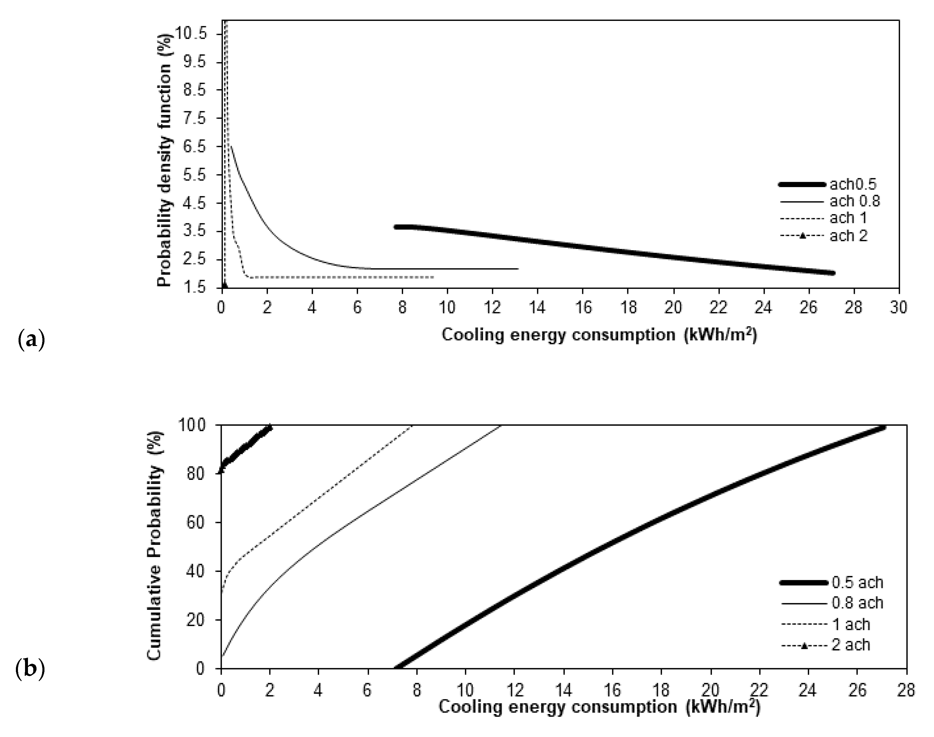
Despite the fact that the summer season is a holiday, cooling systems may be added to classrooms due to the expected need to reduce pandemic infections in this hot period. As a consequence, the cooling energy demand estimated for that period was defined.
From Table 1 and Table 2, it can be concluded that for the heating season, the energy consumption increases when the air changes increase. At the same time, the increment of outdoor temperature implies a reduction of the heating energy. In the cooling season, the energy consumption decreases at the same time that air changes increase. Moreover, it can be observed that energy consumption will increase at the same time that outdoor temperature increases. Despite this, the cooling energy consumption is, overall, reduced for that climatic region. Therefore, it might be interesting to consider changing part of the winter teaching period to the summer season due to the high energy saving and reduced possibility of contagion.
As the aim of this work is to define the optimal moment and the exact increment of the number of air changes to lower energy consumption, this will be solved numerically and by the proposed Weibull model constants. To solve it numerically, two models were obtained by curve fitting from the information shown in Table 1 and Table 2. The first model, Equation (3), is for the heating period (HE) and was obtained with a determination factor of 0.95:
where ACH refers to the air changes (h−1) and Δt is the increase in temperature with regards to the seasonal average value (°C).
When the minimum of this function was solved numerically, a minimum energy consumption of 6.20 kWh/m2 was obtained during the winter when the air changes are 0.52 h−1 and there is an increment of 0.60 °C with respect to the average seasonal value. The maximum of this function, with 77 kWh/m2, was obtained at the average winter temperature and the number of air changes is 2 ach. This maximum energy consumption corresponds with the proposed option to prevent COVID infections during the winter season. As a consequence, since the objective is to increase the number of air changes, the same analysis was done in the summer season to define the cooling energy (CE) model, defined by Equation (4). This model was obtained with a determination factor of 88.15:
where ACH refers to the air changes (h−1) and Δt is the increase in temperature with regards to the seasonal average value (°C).
Based on this cooling model, the minimum energy consumption is identified with an increment of 0.15 °C of the seasonal average temperature and with 1.67 ach air changes. As a consequence, this is the better solution for a compatible increment of air changes in accordance with COVID requirements and a lower energy consumption.
The previous resolution is just a numerical resolution of the problem, but it does not let researchers understand the reason why this is the optimal ventilation period compared to alternative options. As a consequence, an analysis of the Weibull model constants was done.
From Table 1 and Table 2, it can be observed that most of the determination factors present a high value, showing a good agreement between the Weibull model and the probability of energy consumption. In this sense, it can be observed that the constants “e0” and “e1” (shape parameter) can be related with each type of curve and, as a consequence, its corresponding energy consumption. In particular, when the “e” constant reaches a zero value, the curve is exponential and, when it is near to 3.5, a normal distribution is expected and the energy consumption is at a minimum. This is due to that the area below the curve is smaller in a normal distribution with respect to an exponential or a lognormal curve. Finally, if the “e” constant increases to a value over 3.5, the energy consumption tends to increase.
Another interesting conclusion that can be obtained from these tables is that a temperature increase of 0.5 °C or 1 °C in winter season makes the “e0” constant grow towards a normal distribution and, as a consequence, the energy consumption is reduced. The inverse effect is observed in the summer season, when the temperature increase reduces the “e1” value and, as a consequence, increases energy consumption.
Based on this analysis, the optimal ventilation rate is identified when the “e” constant is near 3 in two cases in the summer season. These two cases are at an average outdoor temperature condition and 2 and 1 ach, respectively. As a consequence, these two are the first and second optimal energetic solutions for this problem, since in these cases a normal distribution is expected, and the exact ventilation rate must be selected in accordance with the ventilation needs. It is interesting to highlight that this normal distribution is due to a high number of iterations with a reduced difference between outdoor and indoor conditions. As a consequence, this objective can be obtained with different building design parameters, and can thus function as a new way to guide HVAC operators and designers to produce more optimized buildings.
This result is in agreement with the previous numerical resolution and, as a consequence, it can be concluded that these constants are a good guide to define the conditions with a lower energy consumption in accordance with different requirements.
In our particular case study, it is of interest to the autonomous community of Galicia to calculate the exact energy saving if they do change the teaching periods. In particular, the increase of the heating energy consumption when the air changes increase from their actual 0.8 ach to 2 ach in the winter season. As a consequence, if we employ the more unfavorable increase of energy consumption in the winter season, identified as the highest augmentation in energy consumption defined by Table 1, 57.24 kWh/m2 is obtained. This increase in energy consumption does not reflect a relevant change for any outdoor air temperature increase. If a Heating Ventilation and Air Conditioning system (HVAC) is employed for conditioning the classes in the summer period, an increment of the energy consumption, at the time to increase the air changes from 0.8 ach to 2 ach, of 0.36 kWh/m2 was obtained. As a consequence, it can be concluded that a decrement of the energy consumption of 72.6 kWh/m2 when part of the winter teaching months is replaced to summer teaching months.
Finally, due to that the summer season are mild in the Galicia region and that this calculation considers a HVAC system to cool indoor ambience, if this equipment depreciates because it is not really employed, the energy saving will increase up to 72.96 kWh/m2. As a consequence, changing the teaching months to the summer season and increasing the air changes is an interesting method to reduce the pandemic virus. This will be improved by the fact that in the summer months, a reduced risk of contagion of COVID-19 is expected.
5. Conclusions
In the present paper, a new method to understand building energy consumption and selecting the optimal period to increase the air changes in accordance with different needs is shown. In particular, results showed that the Monte Carlo method applied over ISO 13790 standards are a useful tool to define the probability of building energy consumption. Furthermore, it was obtained that the probability of building energy consumption can be defined by a Weibull model. After analyzing these Weibull model constants, the shape factor “e” lets us identify the conditions at which the probability density function is a normal distribution. This normal distribution is one with a lower energy consumption and can be identified by an “e” of 3.5, which is a useful tool for buildings and HVAC designers.
In particular, this methodology was employed to analyze the case study of energy saving when some teaching periods are changed from winter to summer seasons. It was obtained that, due to the mild Galician climate, this alternative is an adequate proposal to prevent COVID infections.
Author Contributions
Conceptualization, J.A.O., M.K.N., and S.R.; methodology, J.A.O. and M.K.N.; software, S.R.; validation, S.R.; formal analysis, J.A.O. and M.K.N.; investigation, J.A.O., M.K.N., and S.R.; resources, J.A.O., M.K.N., and S.R.; data curation, J.A.O., M.K.N., and S.R.; writing—original draft preparation, J.A.O., M.K.N., and S.R.; writing—review and editing, J.A.O., M.K.N., C.M., and S.R.; visualization, J.A.O., M.K.N., C.M., and S.R.; supervision, J.A.O., M.K.N., and S.R.; project administration, J.A.O., M.K.N., and S.R.; funding acquisition, J.A.O., M.K.N., and S.R. All authors have read and agreed to the published version of the manuscript.
Funding
This research was funded by CYPE Ingenieros S.A. in their research project to reduce energy consumption in buildings and its certification, in collaboration with the University of A Coruña (Spain) (Grant No. 64900).
Acknowledgments
The authors wish to express their acknowledgement to Miguel Orosa García for his advice during the development of this work. Finally, this paper is dedicated to the memory of Antonio Fernández García (ETSNyM, University of A Coruña).
Conflicts of Interest
The authors declare no conflict of interest.
References
- Orosa, J.A.; Oliveira, A.C. An indoor air perception method to detect fungi growth in flats. Expert Syst. Appl. 2012, 39, 3740–3746. [Google Scholar] [CrossRef]
- ASHRAE Indications Reoupening Schools and Universities. Available online: https://www.ashrae.org/technical-resources/reopening-of-schools-and-universities (accessed on 22 September 2020).
- REHVA CO2 Sensor. Available online: https://www.rehva.eu/fileadmin/user_upload/REHVA_COVID-19_guidance_document_V3_03082020.pdf (accessed on 22 September 2020).
- How Covid Travels in Classrooms. Available online: https://cse.umn.edu/college/news/new-study-explores-how-coronavirus-travels-indoors (accessed on 22 September 2020).
- WHO. World Health Organization. Schools. Available online: https://www.who.int/publications/m/item/key-messages-and-actions-for-covid-19-prevention-and-control-in-schools (accessed on 22 September 2020).
- Nematchoua, M.K.; Mempouo, B.; Tchinda, R.; Costa, A.M.; Orosa, J.A.; Raminosoa, C.R.R.; Mamiharijaona, R. Resource potential and energy efficiency in the buildings of Cameroon: A review. Renew. Sustain. Energy Rev. 2015, 50, 835–846. [Google Scholar]
- Nematchoua, M.K.; Tchinda, R.; Orosa, J.A. Thermal comfort and energy consumption in modern versus traditional buildings in Cameroon: A questionnaire-based statistical study. Appl. Energy 2014, 114, 687–699. [Google Scholar] [CrossRef]
- Peng, L.L.H.; Jim, C.Y. Green-Roof Effects on Neighborhood Microclimate and Human Thermal Sensation. Energies 2013, 6, 598–618. [Google Scholar] [CrossRef] [Green Version]
- Jim, C.Y. Thermal performance of climber greenwalls: Effects of solar irradiance and orientation. Appl. Energy 2015, 154, 631–643. [Google Scholar] [CrossRef]
- Setiawan, A.F.; Tzu-Ling, H.; Chun-Ta, T.; Chi-Ming, L. The Effects of Envelope Design Alternatives on the Energy Consumption of Residential Houses in Indonesia. Energies 2015, 8, 2788–2802. [Google Scholar] [CrossRef]
- Parra, J.; Guardo, A.; Egusquiza, E.; Alavedra, P. Thermal Performance of Ventilated Double Skin Façades with Venetian Blinds. Energies 2015, 8, 4882–4898. [Google Scholar] [CrossRef]
- ASHRAE Handbook: HVAC Fundamentals; Spanish Edition, Editorial Index; ASHRAE: Atlanta, GA, USA, 2013; pp. 1–197.
- ISO 13790. Thermal Performance of Buildings-Calculation of Energy Use for Space Heating and Cooling; ISO/DIS 13790:2008; International Organization for Standardization: Geneva, Switzerland, 2008. [Google Scholar]
- International Energy Agency (IEA). Welcome to the International Energy Agency’s Energy in Buildings and Communities Programme. Available online: https://www.iea-ebc.org (accessed on 8 October 2020).
- Haarhoff, J.; Mathews, E.H. A Monte Carlo method for thermal building simulation. Energy Build. 2006, 38, 1395–1399. [Google Scholar] [CrossRef] [Green Version]
- Keirstead, J.; Shah, N. Calculating minimum energy urban layouts with mathematical programming and Monte Carlo analysis techniques. Comput. Environ. Urban Syst. 2011, 35, 368–377. [Google Scholar] [CrossRef] [Green Version]
- Mavrotas, G.; Florios, K.; Vlachou, D. Energy planning of a hospital using Mathematical Programming and Monte Carlo simulation for dealing with uncertainty in the economic parameters. Energy Convers. Manag. 2010, 51, 722–731. [Google Scholar] [CrossRef]
- Gang, W.; Wang, S.; Shan, K.; Gao, D. Impacts of cooling load calculation uncertainties on the design optimization of building cooling systems. Energy Build. 2015, 94, 1–9. [Google Scholar] [CrossRef]
- Ren, X.; Yan, D.; Wang, C. Air-conditioning usage conditional probability model for residential buildings. Build. Environ. 2014, 81, 172–182. [Google Scholar] [CrossRef]
- Lu, Y.; Huang, Z.; Zhang, T. Method and case study of quantitative uncertainty analysis in building energy consumption inventories. Energy Build. 2013, 57, 193–198. [Google Scholar] [CrossRef]
- Srinivasa Rao, A.S.R. On joint Weibull probability density functions. Appl. Math. Lett. 2005, 18, 1224–1227. [Google Scholar] [CrossRef] [Green Version]
- Prabhakar Murthy, D.N.; Bulmer, M.; Eccleston, J.A. Weibull model selection for reliability modelling. Reliab. Eng. Syst. Safe 2004, 86, 257–267. [Google Scholar] [CrossRef]
- MeteoGalicia. Anuario Climatolóxico de Galicia. Consellería de Medio Ambiente. Xunta de Galicia. Available online: https://www.meteogalicia.gal/observacion/informesclima/informesIndex.action?request_locale=es (accessed on 13 October 2020).
- Orosa, J.A.; Oliveira, A.C. Implementation of a method in EN ISO 13790 for calculating the utilisation factor taking into account different permeability levels of internal coverings. Energy Build. 2010, 42, 598–604. [Google Scholar] [CrossRef]
- Orosa, J.A.; García-Bustelo, E.J. Permeable coverings as a sustainable solution for indoor air thermal comfort and energy saving. Energy Edu. Sci. Technol. A 2012, 29, 583–596. [Google Scholar]
- Masdias-Bonome, A.E.; Orosa, J.A.; Vergara, D. A New Methodology for Decision-Making in Buildings Energy Optimization. Appl. Sci. 2020, 10, 4558. [Google Scholar] [CrossRef]
- Šadauskienė, J.; Paukštys, V.; Šeduikytė, L.; Banionis, K. Impact of Air Tightness on the Evaluation of Building Energy Performance in Lithuania. Energies 2014, 7, 4972–4987. [Google Scholar] [CrossRef] [Green Version]
- Fei, F.; Zhou, S.; Mai, J.D.; Li, W.J. Development of an Indoor Airflow Energy Harvesting System for Building Environment Monitoring. Energies 2014, 7, 2985–3003. [Google Scholar] [CrossRef] [Green Version]
- Nematchoua, M.K.; Tchinda, R.; Orosa, J.A.; Andreasi, W.A. Effect of wall construction materials over indoor air quality in humid and hot climate. J. Build. Eng. 2015, 3, 16–23. [Google Scholar] [CrossRef] [Green Version]
- Karlsson, F.; Fahlén, P. Impact of design and thermal inertia on the energy saving potential of capacity controlled heat pump heating systems. Int. J. Refrig. 2008, 31, 1094–1103. [Google Scholar] [CrossRef]
- Mazarrón, F.R.; Cid-Falceto, J.; Cañas, I. Ground Thermal Inertia for Energy Efficient Building Design: A Case Study on Food Industry. Energies 2012, 5, 227–242. [Google Scholar] [CrossRef]
- Orosa, J.A. Thermal inertia and ISO 13790—Have its effects on future energy consumption been fully considered? Energy Edu. Sci. Technol. 2012, 29, 339–352. [Google Scholar]
- Orosa, J.A.; Oliveira, A.C. A field study on building inertia and its effects on indoor thermal environment. Renew. Energy 2012, 37, 89–96. [Google Scholar] [CrossRef]
- MeteoGalicia. Xunta de Galicia. Consellería de Medio ambiente Teorritorio e Vivenda. Available online: https://www.meteogalicia.gal/datosred/infoweb/clima/informes/estacions/anuais/2019_es.pdf (accessed on 22 September 2020).
Publisher’s Note: MDPI stays neutral with regard to jurisdictional claims in published maps and institutional affiliations. |
Figure 1.
Typical school building plant.

Figure 2.
Histogram of energy consumption during the heating season.

Figure 3.
Probability density functions (a) and cumulative probability (b) of the heating energy consumption for different air changes (Ach = 0.5, Ach = 0.8, Ach = 1.0, Ach = 2.0).
Figure 3.
Probability density functions (a) and cumulative probability (b) of the heating energy consumption for different air changes (Ach = 0.5, Ach = 0.8, Ach = 1.0, Ach = 2.0).

Figure 4.
Probability density functions (a) and cumulative probability (b) of the heating energy consumption for an increment of +0.5 °C in the outdoor temperature.
Figure 4.
Probability density functions (a) and cumulative probability (b) of the heating energy consumption for an increment of +0.5 °C in the outdoor temperature.

Figure 5.
Probability density functions (a) and cumulative probability (b) of the heating energy consumption for an increment of +1 °C in the outdoor temperature.
Figure 5.
Probability density functions (a) and cumulative probability (b) of the heating energy consumption for an increment of +1 °C in the outdoor temperature.

Figure 6.
Probability density functions (a) and cumulative probability (b) of the cooling energy consumption for different air changes (Ach = 0.5, Ach = 0.8, Ach = 1.0, Ach = 2.0).
Figure 6.
Probability density functions (a) and cumulative probability (b) of the cooling energy consumption for different air changes (Ach = 0.5, Ach = 0.8, Ach = 1.0, Ach = 2.0).

Figure 7.
Probability density functions (a) and cumulative probability (b) of the cooling energy consumption for an increment of +0.5 °C in the outdoor temperature.
Figure 7.
Probability density functions (a) and cumulative probability (b) of the cooling energy consumption for an increment of +0.5 °C in the outdoor temperature.

Figure 8.
Probability density functions (a) and cumulative probability (b) of the cooling energy consumption for an increment of +1 °C in the outdoor temperature.
Figure 8.
Probability density functions (a) and cumulative probability (b) of the cooling energy consumption for an increment of +1 °C in the outdoor temperature.


Table 1.
Curve fitting of probability density function during the heating season.
| Average Heating Energy Consumption (kWh/m2) | ACH (h−1) | Outdoor Temp. (°C) | a0 | b0 | c0 | d0 | e0 | r2 |
|---|---|---|---|---|---|---|---|---|
| 5.44 | 0.5 | Average | 3.363271 | 2.661263 | 9.437849 | 1.011474 | 0 | 0.92 |
| 5.10 | 0.5 | +0.5 °C | 1.854899 | 2.080979 | 2.565297 | 2.295291 | 1.007102 | 0.97 |
| 4.80 | 0.5 | +1 °C | 1.854899 | 2.080979 | 2.565297 | 2.295291 | 1.007102 | 0.97 |
| 15.72 | 0.8 | Average | 3.090611 | 8.386542 | 32.028872 | 1.010309 | 0 | 0.93 |
| 15.68 | 0.8 | +0.5 °C | 3.304539 | 8.415014 | 29.33913 | 1.012122 | 0 | 0.90 |
| 15.65 | 0.8 | +1 °C | 3.124542 | 8.369421 | 30.40935 | 1.010302 | 0 | 0.90 |
| 46.97 | 1.0 | Average | 3.212779 | 13.38395 | 42.19215 | 1.010308 | 0 | 0.91 |
| 24.20 | 1.0 | +0.5 °C | 3.077777 | 13.48641 | 45.60571 | 1.011666 | 0 | 0.92 |
| 22.19 | 1.0 | +1 °C | 3.050013 | 13.48202 | 45.16667 | 1.011673 | 0 | 0.92 |
| 72.96 | 2.0 | Average | 2.882833 | 46.047900 | 162.5114 | 1.012475 | 0 | 0.85 |
| 70.25 | 2.0 | +0.5 °C | 1.512973 | 1.519573 | 48.13923 | 39.73227 | 1.093759 | 0.91 |
| 68.92 | 2.0 | +1 °C | 1.862788 | 1.223835 | 47.25478 | 30.64512 | 1.095933 | 0.94 |
Table 2.
Curve fitting of probability density function during the cooling season.
| Average Cooling Energy Consumption (kWh/m2) | ACH (h−1) | Outdoor Temp. (°C) | a1 | b1 | c1 | d1 | e1 | r2 |
|---|---|---|---|---|---|---|---|---|
| 15.97 | 0.5 | Average | 2.794215 | 2.479324 | 8.207154 | 5.324309 | 1.06168 | 0.91 |
| 16.34 | 0.5 | +0.5 °C | 3.618063 | 7.566651 | 29.62327 | 1.013869 | 0 | 0.83 |
| 16.94 | 0.5 | +1 °C | 3.273713 | 7.46334 | 24.62232 | 1.0127 | 0 | 0.84 |
| 5.30 | 0.8 | Average | 3.668553 | 9.12329 | −2.019566 | 3.309106 | 1.0585379 | 0.95 |
| 5.45 | 0.8 | +0.5 °C | 3.273713 | 7.46334 | 24.62232 | 1.0127 | 0 | 0.84 |
| 5.52 | 0.8 | +1 °C | 1.973009 | 4.136657 | 0.203551 | 1.313985 | 1.085427 | 0.81 |
| 1.18 | 1.0 | Average | 2.734177 | 3321.353 | −3.61981 | 3.85073 | 3.236254 | 0.99 |
| 3.16 | 1.0 | +0.5 °C | 3.077777 | 13.48641 | 45.60571 | 1.011666 | 0 | 0.92 |
| 4.38 | 1.0 | +1 °C | 3.050013 | 13.48202 | 45.16667 | 1.011673 | 0 | 0.92 |
| 0.36 | 2.0 | Average | 1.449848 | 347.4151 | −0.27093 | 0.463775 | 3.049235 | 0.99 |
| 1.15 | 2.0 | +0.5 °C | 1.512973 | 1.519573 | 48.13923 | 39.73227 | 1.093759 | 0.91 |
| 1.19 | 2.0 | +1 °C | 0.447502 | 149105.2 | −0.3577 | 1.293282 | 10.01984 | 0.99 |
© 2020 by the authors. Licensee MDPI, Basel, Switzerland. This article is an open access article distributed under the terms and conditions of the Creative Commons Attribution (CC BY) license (http://creativecommons.org/licenses/by/4.0/).
Share and Cite
MDPI and ACS Style
Orosa, J.A.; Kameni Nematchoua, M.; Reiter, S. Air Changes for Healthy Indoor Ambiences under Pandemic Conditions and Its Energetic Implications: A Galician Case Study. Appl. Sci. 2020, 10, 7169. https://doi.org/10.3390/app10207169
AMA Style
Orosa JA, Kameni Nematchoua M, Reiter S. Air Changes for Healthy Indoor Ambiences under Pandemic Conditions and Its Energetic Implications: A Galician Case Study. Applied Sciences. 2020; 10(20):7169. https://doi.org/10.3390/app10207169
Chicago/Turabian StyleOrosa, José A., Modeste Kameni Nematchoua, and Sigrid Reiter. 2020. "Air Changes for Healthy Indoor Ambiences under Pandemic Conditions and Its Energetic Implications: A Galician Case Study" Applied Sciences 10, no. 20: 7169. https://doi.org/10.3390/app10207169
Note that from the first issue of 2016, this journal uses article numbers instead of page numbers. See further details here.