
Ensemble Deep Learning for the Detection of COVID-19 in Unbalanced Chest X-ray Dataset


1
King Mongkut’s Institute of Technology Ladkrabang, School of Engineering, Bangkok 10520, Thailand
2
School of Information and Telecommunication Engineering, Tokai University, Tokyo 108-8619, Japan
*
Author to whom correspondence should be addressed.
Appl. Sci. 2021, 11(22), 10528; https://doi.org/10.3390/app112210528
Submission received: 29 September 2021
/
Revised: 23 October 2021
/
Accepted: 3 November 2021
/
Published: 9 November 2021
(This article belongs to the Special Issue Advanced Intelligent Imaging Technology Ⅲ)
Abstract
:The ongoing COVID-19 pandemic has caused devastating effects on humanity worldwide. With practical advantages and wide accessibility, chest X-rays (CXRs) play vital roles in the diagnosis of COVID-19 and the evaluation of the extent of lung damages incurred by the virus. This study aimed to leverage deep-learning-based methods toward the automated classification of COVID-19 from normal and viral pneumonia on CXRs, and the identification of indicative regions of COVID-19 biomarkers. Initially, we preprocessed and segmented the lung regions usingDeepLabV3+ method, and subsequently cropped the lung regions. The cropped lung regions were used as inputs to several deep convolutional neural networks (CNNs) for the prediction of COVID-19. The dataset was highly unbalanced; the vast majority were normal images, with a small number of COVID-19 and pneumonia images. To remedy the unbalanced distribution and to avoid biased classification results, we applied five different approaches: (i) balancing the class using weighted loss; (ii) image augmentation to add more images to minority cases; (iii) the undersampling of majority classes; (iv) the oversampling of minority classes; and (v) a hybrid resampling approach of oversampling and undersampling. The best-performing methods from each approach were combined as the ensemble classifier using two voting strategies. Finally, we used the saliency map of CNNs to identify the indicative regions of COVID-19 biomarkers which are deemed useful for interpretability. The algorithms were evaluated using the largest publicly available COVID-19 dataset. An ensemble of the top five CNNs with image augmentation achieved the highest accuracy of 99.23% and area under curve (AUC) of 99.97%, surpassing the results of previous studies.
1. Introduction
COVID-19 is a contagious disease caused by severe acute respiratory syndrome coronavirus (SARS-CoV-2). It affects people differently: most infected people will experience mild to moderate illness and recover without hospitalization and special treatment; however, some will become severely ill and need immediate medical treatment. COVID-19 can attack the upper respiratory airways and often exhausts the infected person’s immune system. Many infected people suffer short-term and long-term side effects. As of September 2021, COVID-19 has infected more than 220 million people worldwide, and more than 4 million people have died as a result of infection. Figure 1 shows the number of COVID-19-related cases and fatalities by territory and area [1,2].
Researchers around the world are intensively working on the development of accurate and reliable diagnostic tools, medical treatments, and necessary vaccines to prevent the virus from spreading, and to eventually eradicate it. Our work contributes to the development of accurate and reliable diagnostic tests. Real-time reverse transcription-polymerase chain reaction (RT-PCR) assays are used as the standard test for COVID-19 diagnosis. However, it is a time-intensive and complex process, and not widely available in some geographic regions, especially in rural communities of developing countries. Medical images such as computed tomography (CT) scans and CXRs are vital for the early diagnosis and treatment of COVID-19 and represent the main clinical resources to evaluate the extent of lung damage caused by COVID-19 [3,4]. COVID-19 patients exhibit several unique clinical and para-clinical features on radiology images, such as reciprocal, multi-focal, ground-glass opacities with a fringe or back-dissemination in the early stage, and pulmonary consolidation in the late stage. Some studies have encountered changes in CXR and CT images before the onset of COVID-19 symptoms [5]. Although CT is a sensitive technique to diagnose COVID-19 and provides greater resolution, it is a cost-intensive and highly radiating technique that carries a high risk of cross-infection among medical experts and necessitates intensive sterilization of the apparatus [6]. In contrast to CTs, CXRs are less costly and inflict a lower radiation dose and are easier to obtain without risking contamination of the imaging equipment. The imaging process can be performed with portable X-ray machines at the patient’s bedside. X-ray imaging machines are ubiquitously available worldwide and almost all hospitals have these machines; therefore, CXRs can be used to screen or triage COVID-19 without dedicated test kits, thus not incurring any overhead operational costs for data collection. Hence, CXR imagery has become a key tool to screen or triage COVID-19 patients and plays a vital role in the evaluation of lung deterioration incurred by COVID-19 [4,7].
The manual examination of CXRs is a time-intensive and subjective task and needs a high degree of expertise. There is a shortage of trained radiologists in many healthcare systems, especially in developing countries and remote areas. COVID-19 pneumonia may have similar pathology patterns with non-COVID-19 pneumonia; therefore, it is hard to discern COVID-19 CXRs from those of pneumonia, requiring extra time commitments and thereby exacerbating the shortage of competent medical experts. Moreover, COVID-19 has exhausted and caused a strain on medical experts [8]. Health services have been used to the fullest extent and sometimes to the brink of collapse due to the pandemic. These concerns necessitate the development of accessible and feasible innovative systems. With the advent of artificial intelligence (AI) and computer vision techniques, AI-assisted tools have become an adjunct tool for clinicians. They can serve as a complementary tool to human readings of medical images and aid the medical personnel in diagnoses. Thus, efficient and accurate AI-assisted tools are urgently needed to facilitate medical experts in COVID-19 diagnosis and expedite mass testing programs in high-risk areas, where many chest medical scans need to be examined. This study aimed to develop accurate and effective algorithms for the classification of COVID-19, normal, and pneumonia on CXRs using deep learning.
1.1. Related Works
Remarkable progress has been made in the automated detection of COVID-19 in CXRs [9,10,11,12,13,14,15,16,17,18,19,20,21,22,23,24]. Several studies in the literature have leveraged deep convolutional neural networks (CNNs) with and without modifications to convincingly predict COVID-19. CNNs are end-to-end learning models that use multiple processing layers to learn and discover classification patterns and features without explicitly extracting the hand-crafted features. In general, there are two types of classification—binary classification and multi-classification—to predict the prevalence of COVID-19 in CXRs. Binary classification aims to discriminate between positive and negative cases of COVID-19 [10,11,12,13,14]. Nevertheless, binary classification can lead to the misclassification of COVID-19 with other lung diseases such as non-COVID-19 pneumonia, bacterial pneumonia, and tuberculosis (TB). To remedy this issue, researchers have applied multi-classification of COVID-19 from normal, bacterial pneumonia, TB. Multi-classification methods have improved the detection accuracy of COVID-19 [9].
Hemdan et al. [10] presented deep learning-based COVIDX-Net using seven CNNs to distinguish positive COVID-19 CXRs from negative ones and obtained an F-measure of 89% for normal and 91% for COVID-19 on a dataset of 25 normal and 25 COVID-19 CXRs. However, their dataset is relatively small to build a reliable deep learning-based model. Sahlol et al. [11] presented a hybrid classifier that uses the pretrained InceptionNet model as a feature extractor and marine predators’ algorithms as the feature selection method to find the dominant features among all extracted features. They achieved 98.7% accuracy on dataset1 consisting of 200 COVID-19 positive CXRs and 1675 CXRs, and 99.6% accuracy on dataset2 consisting of 219 COVID-19 positive and 1341 negative COVID-19 CXRs. Alazab et al. [12] utilized VGG-19 based COVID-19 detection with and without image augmentation. Their algorithm attained 95% of F-measure on the original dataset consisting of 28 healthy and 70 COVID-19, and 99% of F-measure on the augmented dataset consisting of 500 healthy and 500 COVID-19 CXRs. Duran-Lopez et al. [13] proposed a deep learning-based COVID_XNet to differentiate between COVID-19 and normal CXRs and to visualize the COVID-19 pathologies. They first applied a set of image preprocessing techniques such as histogram matching, bone suppression, and contrast limited histogram equalization to reduce the image variability and enhance the image quality. Then, the preprocessed images were input to a customized deep learning architecture to identify COVID-19 CXRs. Their proposed algorithm claimed accuracy of 94.43% and AUC of 98.8% on a dataset consisting of 2589 COVID-19 and 4337 normal CXRs. Khasawneh et al. [14] presented the customized CNN, VGG-16, and MobileNet based classifiers to distinguish COVID-19 from normal CXRs. They claimed the accuracy of 98.7% on the combined public and local dataset containing 1210 COVID-19 and 1583 normal CXRs.
Several multi-classifications of COVID-19 from normal, pneumonia, and TB have been developed using deep CNNs [15,16,17,18,19,20,21]. Wang et al. [15] first introduced an open-source COVID-Net to identify COVID-19 CXRs using a customized CNN model. Using the COVIDx dataset consisting of CXRs from 266 COVID-19 cases, 8066 normal cases and 5538 cases of non-COVID-19 pneumonia patients, they claimed that COVID-Net achieved a sensitivity of over 80%. Brunese et al. [16] presented a VGG-16-based three-fold framework. The first fold classifies between normal and pneumonia CXRs using 3520 healthy and 3003 CXRs of pulmonary diseases, obtaining an accuracy of 96%. Then, the second fold is applied to differentiate COVID-19 pneumonia from non-COVID-19 pneumonia using 250 COVID-19 CXRs and 2753 CXRs of lung diseases, obtaining an accuracy of 98%. The third fold is subsequently carried out to localize the areas of COVID-19 pathologies using Gradient Class Activation Map (Grad-CAM). Ahmed et al. [17] proposed ReCoNet (residual image-based COVID-19 detection network) to classify COVID-19 CXRs from normal and non-COVID-19 pneumonia. ReCoNet is a deep learning framework that applies multi-level filtering blocks for preprocessing images followed by multilevel feature extraction layers and classification layers. Their proposed network was evaluated using a combined dataset consisting of 238 COVID-19, 8851 normal, and 6045 pneumonia CXRs, and attained an overall accuracy of 97.48%. Yoo et al. [18] introduced a deep-learning-based decision tree classifier to recognize COVID-19 CXRs from normal and pneumonia images. The first tree classified between normal and abnormal on a dataset of 585 normal and 585 abnormal CXRs and obtained an accuracy of 98%. The second decision tree further differentiated the abnormal CXRs into TB or non-TB on a dataset consisting of 492 images per class and achieved an accuracy of 80%. The final decision tree differentiated between COVID-19 and TB on a dataset of 142 images per class and attained an average accuracy of 95%. Ozturk et al. [19] presented a variant of the Darknet-19 model with fewer layers and filters to automatically predict COVID-19. Their model was trained as a binary classifier (COVID-19 vs. no findings) and a multi-class classifier (COVID-19 vs. non-findings and pneumonia). Using the dataset consisting of 125 COVID-19, 500 normal, and 500 pneumonia CXRs, the binary classifier achieved 98.08% accuracy, whereas the multi-class classifier achieved 87.02%. Ben Jabra et al. [20] compared the performance of 16 pretrained CNN models and combined the best-performing methods as an ensemble classifier to enhance the accuracy. They achieved the highest accuracy of 99% with the ensemble classifier by using majority voting on the dataset of 237 COVID-19, 1338 normal, and 1336 viral pneumonia CXRs. Shelke et al. [21] presented a three-stage COVID-19 detection and severity scoring metric. The first stage used VGG-16 to differentiate between normal, pneumonia and TB, and achieved 95.9% accuracy. Then, the second stage further classified the pneumonia CXRs into COVID-19 pneumonia and non-COVID-19 pneumonia using DenseNet-161, obtaining 98.9% accuracy. The final stage used ResNet-18 to grade the COVID-19 pneumonia CXRs into mild, medium, and severe, with a test accuracy of 76%. Except for [13,14], previous studies have applied deep learning on the dataset with a very limited number of COVID-19 CXRs, fewer than 300 images. Deep learning algorithms need massive amounts of data to learn the information and patterns for classification; therefore, using a small dataset might hinder the efficiency of these studies.
To mitigate the problem of a limited number of COVID-19 CXRs, Oh et al. [22] and Rajaraman et al. [23] proposed algorithms which work well with limited datasets. Oh et al. [22] proposed a patch-based deep learning method for the classification of COVID-19 CXRs from normal, non-COVID-19 pneumonia and TB images on a limited training dataset. Initially, the images are preprocessed, and subsequently, lung regions are segmented using FC-DenseNet. The segmented images are partitioned into small patches and fed to ResNet-18 to predict COVID-19. Finally, the heat saliency maps are superimposed on the segmented lung regions to spot biomarkers. Their algorithm was assessed on a combined dataset of six public datasets consisting of 180 COVID-19, 191 normal, 74 pneumonia and 57 TB CXRs, and attained a sensitivity of 92.5%. For multi-classification of COVID-19, pneumonia, and normal CXRs, Rajaraman et al. [23] presented several fine-tuned CNNs which were optimized with the grid search method. Lung regions were segmented and cropped using U-Net segmentation. The models were then iteratively pruned to reduce the model complexity and to deal with the limited number of images. Finally, the best-performing pruned models were combined as the ensemble classifier. Their ensemble model yielded an average accuracy of 99.01% on a combined dataset of four public datasets with 313 COVID-19, 7595 normal, and 8792 pneumonia CXRs. An exception to the neglect of unbalanced data problems by previous studies, Bridge et al. [24] presented the generalized extreme value (GEV) as the activation function of InceptionNet to handle the highly imbalanced dataset of 129 COVID-19, 5689 pneumonia, and 62,267 healthy CXRs. Compared to the classic sigmoid activation function, InceptionNet with GEV function produced better accuracy by giving an AUC of 82% on binary classification between healthy and COVID-19 and attained 73.1% AUC on the multi-classification of healthy, pneumonia, and COVID-19 images. Nishio et al. [25] proposed a VGG-16 based computer aided diagnosis system to classify COVID-19 pneumonia, non-COVID-19 pneumonia, and healthy CXRs. To prevent overfitting, they applied a composite of conventional data augmentation and mixup method on the original dataset and input it to VGG-16 for transfer learning. Their proposed method is evaluated using a dataset consisting of 215 COVID-19 pneumonia, 533 non-COVID-19 pneumonia, and 500 healthy CXRs extracted from two public datasets, and obtained the accuracy of 83.6% of three-category classification and over 90% sensitivity for COVID-19 pneumonia.
1.2. Our Contributions
From the above section, it has been shown that the limitations of the previous studies lay in three aspects: using whole CXRs, using datasets with limited availability of COVID-19 CXRs, and using highly unbalanced datasets. Most previous studies, except for [22,23], directly used the whole image without lung segmentation. CXRs contain regions other than lungs, which are irrelevant for the classification of COVID-19 from normal and pneumonia. The irrelevant regions present in the images can mislead the decision-making of CNN models and increase the computational time. Moreover, the dataset used in this study was a heterogeneous dataset curated from many different sources, such as hospitals, healthcare centers, published journals, and articles. Some COVID-19 CXRs in the dataset contain labels, texts, and pointing arrows. Deep CNNs learn from the distinguished features of images for each class; foreign and irrelevant signs may cause misclassification because only COVID-19 CXRs contain these signs. It is of the utmost importance to segment lung regions from whole CXRs. In this study, we utilized deep semantic algorithms to segment the lungs to maximize the prediction capacity of CNNs and minimize the computational time. Another major bottleneck of most prior studies is the limited availability of COVID-19 CXRs. Training data-hungry deep learning models using a small dataset will underfit the models. Another limitation that hinders the effectiveness of the previous studies is unbalanced class distribution, which can cause biased classification results. We utilized five different approaches which are alternatives to the method proposed by Bridge et al. [24], to handle the unbalanced data. In summary, the main contributions of this study can be elaborated as follows:
- Performing lung segmentation before the classification of diseases;
- Applying five different approaches which are simple, easy to implement and reproduce, yet effective, to tackle unbalanced class distribution;
- Evaluating and validating the presented algorithms using the dataset with the largest number of COVID-19 CXRs;
- Visualizing the indicative regions that highly influence CNNs’ prediction, which are deemed useful for interpretability and explainability.
First, we preprocessed the images using filtering and image enhancement. The preprocessed images were then input to DeepLabV3+ segmentation algorithm to segregate the lung regions from the whole CXRs. The cropped lung regions were then used as inputs to the classification of COVID-19 from normal and pneumonia CXRs using the deep learning methods. To overcome the unbalanced class distribution, we applied five different approaches: (i) weighted loss; (ii) image augmentation; (iii) undersampling; (iv) oversampling; and (v) hybrid sampling. The best-performing models from each approach were then combined as the ensemble classifier using voting strategies to improve the prediction accuracy. We found that an ensemble of CNNs with image augmentation achieved the highest accuracy of 99.23% and AUC of 99.97%. Finally, Grad-CAM was used to identify the indicative regions of COVID-19 biomarkers.
2. Dataset Description
In this study, we utilized version 2 of the COVID-19 Radiography Database which is the winner of COVID-19 Dataset Award by the Kaggle community [26,27]. The dataset was created, curated and made public by a group of researchers from Qatar University, Doha, and the University of Dhaka, Bangladesh, along with their collaborators from Pakistan and Malaysia in collaboration with medical doctors [26,27]. The dataset is publicly accessible at https://www.kaggle.com/tawsifurrahman/covid19-radiography-database (accessed on 30 May 2021). We acquired a total of 15,153 CXR images consisting of 10,192 normal, 3616 COVID-19, and 1345 pneumonia CXRs from the dataset. Figure 2 shows the example CXRs from the dataset, and Table 1 presents the description of the dataset.
3. Methodology
In this study, we propose ensemble deep-learning-based COVID-19 predictions from CXRs. Figure 3 presents a block diagram of the proposed study. Initially, image preprocessing was performed to reduce image variability and noise and enhance the contrast of the images. Lung segmentation was carried out using DeepLabV3+ semantic algorithm. The lung regions were cropped using the lung masks and inputted to deep learning models to classify COVID-19 CXRs from normal and pneumonia images. At first, we applied transfer learning of CNN models to classify CXRs. However, the dataset was highly unbalanced; therefore, we applied five different approaches: (i) class loss weighting; (ii) image augmentation; (iii) undersampling; (iv) oversampling; and (v) hybrid sampling, to prevent biased classifications. The best-performing models from each approach were combined as the ensemble classifier to improve the prediction accuracy. Finally, the indicative regions of COVID-19 lesions were detected by deep learning for better interpretability.
3.1. Image Preprocessing
Image preprocessing is a prerequisite in medical image analysis. It greatly influences lung segmentation and classification results [28]. The dataset we used was curated from many sources; therefore, it presents large variability among the images and contains some with noise and some with blurred contrast. Hence, we performed image preprocessing to normalize image variability and enhance the image quality. First, noise elimination was performed using a median filter, which is a nonlinear filter which reduces noise and preserves edges [29]. Then, the contrast of the image was enhanced using contrast-limited adaptive histogram equalization (CLAHE) [30]. Figure 4 shows the image preprocessing procedure.
3.2. Lung Segmentation
Segmentation is an essential step toward medical image analysis. It is used to separate the region of interest (ROI) from other less relevant regions. For the prediction of COVID-19, lung regions are considered as ROIs because COVID-19 deteriorates the lungs. Hence, we performed image segmentation to segment and crop the lung regions from the whole CXRs. In our previous study of TB detection from CXRs [31], we observed and compared several deep semantic segmentation methods for lung segmentation and found that DeepLabV3+ [32] semantic segmentation performed better than other segmentation methods. Thus, we applied the DeepLabV3+ algorithm with the XceptionNet [33] backbone to segment the lung pixels from CXRs. Figure 5 shows the lung segmentation process. DeepLabV3+ used the preprocessed CXRs as the inputs and generated lung masks as the outputs. Morphological closing and opening [34] were then used to fill the small holes in the mask and refine the boundaries. Using the areas and coordinates of the refined lung mask, we cropped the lung regions from CXRs.
3.3. Classification of COVID-19, Normal and Pneumonia Using Deep Convolutional Neural Networks
After lung regions were cropped from whole CXRs, the cropped images were used as inputs to deep CNNs to distinguish COVID-19 CXRs from normal and pneumonia images. A CNN (or ConvNet) is a specific deep learning architecture that learns from data directly without explicitly extracting the manual features. Building a CNN from scratch needs intensive computational and data resources and can lead to poor performance and overfitting on the small datasets. Another option to apply CNN is fine-tuning pretrained CNNs with transfer learning, which requires smaller datasets and fewer computational resources. Transfer learning is a type of deep learning approach in which a model that has been trained for one task is used as a starting point for a model that performs a similar task. In our study, fine-tuning the CNN models with transfer learning was carried out by transferring the weights of the pretrained network trained on millions of natural images to learn the pattern of CXRs. We employed 11 state-of-the-art deep CNNs as the pretrained models: (i) InceptionV3 [35], (ii) VGG-16, (iii) VGG-19 [36], (iv) XceptionNet [33], (v) ResNet-50 [37], (vi) ResNet-152 [37], (vii) MobileNet [38], (viii) DenseNet201 [39], (ix) InceptionResNetV2 [40], (x) EfficientNetB7 [41], and (xi) NasNetMobile [42], which were trained on ImageNet. For more details on the architectures of these CNN models, please refer to Appendix A. On top of each base model, we added a global pooling layer and sigmoid activation function to create a new fully-connected layer. The new fully-connected layer was trained on the training dataset of cropped lung images to classify between COVID-19, normal, and pneumonia. The categorical cross-entropy loss along with the Adam optimizer is used for fine-tuning the models. The categorical cross-entropy loss is used for multi-class classification and can be formatted as in Equation (1).
where T and N are the training set and its size, respectively. is the predicted probability outputs of the model for i-th samples, and is the corresponding ground-truth label. denotes the number of classes or categories. Fine-tuning CNNs models using normal categorical cross-entropy loss is regarded as Approach 0.
A problem we encountered was the unbalanced class distribution. Figure 6 plots the class distribution of the dataset. The plot shows that it is a heavily unbalanced dataset, where normal CXRs are abundant and COVID-19 and pneumonia CXRs are relatively scarce compared to it. Fine-tuning pretrained CNNs with unbalanced datasets will cause bias in the classification. It is likely to favor the majority class. To remedy the unbalanced data, we applied five simple approaches: (i) Approach 1: training CNNs with the weighted loss, (ii) Approach 2: image augmentation, (iii) Approach 3: undersampling, (iv) Approach 4: oversampling, and (v) Approach 5: hybrid sampling.
3.3.1. Approach 1: Deep Learning with Weighted Loss on an Unbalanced Dataset
Pretrained CNNs were trained on the normal cross-entropy loss to backpropagate the errors, minimizing the loss. However, using a normal cross-entropy loss with our highly unbalanced dataset will incentivize the models to prioritize the majority class, because it contributes more to the loss. Simply put, the majority class will dominate the loss. Therefore, training the deep learning models with a uniformly balanced dataset is preferred so that the positives and negatives of each training class would have an equal contribution to the loss. The first approach to balance the class distribution without altering or transforming the original dataset is to modify the loss of the CNN models. Here, we substituted the cross-entropy loss with the weighted loss to handle the unbalanced dataset. Figure 7 presents a classification of normal, pneumonia, and COVID-19 using CNN models with the weighted cross-entropy loss. The weighted loss will be replaced as the loss of every 11 pretrained CNNs.
In this approach, we applied weighting the loss on the one-class learning strategy for each class in which the samples of the particular class are considered as positive and all other samples as negatives. Suppose we would utilize the cross-entropy loss for prediction of each class: the loss of deep CNNs on the ith training sample can be formulated as Equation (2).
where and are the input features extracted from the pretrained CNNs and the label, and is the prediction output of CNN, i.e., the predicted probability value of a certain class. For every training image, either or . Therefore, only one among these terms has the contribution to the loss and the other term is multiplied by zero and becomes zero [43]. The overall cross-entropy loss for the whole training dataset T of size N can be formatted as in Equation (3).
From the above equation, it can be seen that, if the training set is largely unbalanced with a small number of positive class, the negative class will dominate the loss. The contribution of each class (i.e., positive or negative) can be computed as a summation of the contribution over all the training cases for each class, in Equations (4) and (5) [43]. As shown in Figure 8a, the contribution of each class varies significantly and is unbalanced, especially in COVID-19 and pneumonia classes.
To equalize the contribution of loss for each class, we balanced the contribution of positive and negative labels using weighted loss, which was computed by multiplying each example from each class by a class-specific weight factor, and . To ensure that the overall loss contribution of each class was equal, we performed Equation (6). The weight of each class could be computed using Equations (7) and (8). The weighted cross-entropy for each training sample is defined as Equation (9). Figure 8b plots the equally contributed frequency of each class after loss-weighting. It shows that when using the weighted loss, the positive and negative labels within each class would have the same aggregate contribution to the loss function [43].
The weighted loss computed above is substituted in the place of cross-entropy loss for fine-tuning 11 CNN models.
3.3.2. Approach 2: Deep Learning with Image Augmentation on an Unbalanced Dataset
Another simple and effective approach to handling the unbalanced class distribution is image augmentation. It is used to increase the number of images of the minority classes for training a model. Deep CNN models need a sufficient number of images with an evenly balanced dataset to make reliable predictions. Data augmentation can prevent the overfitting of CNNs as well. Figure 9 shows the flowchart for deep learning with image augmentation on an unbalanced dataset. The number of pneumonia and COVID-19 CXRs are relatively small compared to normal CXRs; therefore, we proportionally applied simple image augmentation methods such as rotation, flipping, shearing, and shifting to increase the number of images in the minority class. The augmented image examples are given in Figure 10. Only the images in the training dataset are augmented. Using the augmented training dataset, 11 CNNs are fine-tuned using categorical cross entropy loss as described in Section 3.3.
3.3.3. Approach 3: Deep Learning with Undersampling on an Unbalanced Dataset
Another naive approach to address the unbalanced class problem is random resampling. One such resampling technique is undersampling. Undersampling randomly selects the samples from the majority class, in our cases, normal CXRs, and deletes them from the training dataset until a more balanced data distribution is achieved. The purpose of resampling here is to influence the fit of the CNNs; therefore, undersampling is only applied to the training dataset [44,45]. In our cases, the normal class had the most images whereas the pneumonia class had the fewest images. We intended to resample normal and COVID-19 CXRs to balance with the pneumonia class. Therefore, we randomly discarded the samples from normal and COVID-19 classes until the normal class was nearly balanced with the pneumonia class. The flowchart of the undersampling approach is illustrated in Figure 11. Using the undersampled training dataset, 11 CNNs are fine-tuned using categorical cross entropy loss as described in Section 3.3.
3.3.4. Approach 4: Deep Learning with Oversampling on an Unbalanced Dataset
In contrast to undersampling, oversampling randomly selects samples from minority classes and then duplicates them. This process is repeated until the more desirable balanced class distribution is reached. COVID-19 and pneumonia were minority classes in our dataset; therefore, we performed oversampling on these two classes until they were nearly equal to the normal class [44,45]. As mentioned in undersampling, oversampling was also applied to the training dataset in order to fit the model. The flowchart of the oversampling approach is depicted in Figure 12. Using the oversampled training dataset, 11 CNNs are fine-tuned using categorical cross entropy loss as described in Section 3.3.
3.3.5. Approach 5: Deep Learning with Hybrid Sampling on an Unbalanced Dataset
The undersampling approach may discard valuable images and lose invaluable information while resampling. On the other hand, oversampling may cause overfitting and could increase the computation effort if a higher oversampling rate is applied. The combination of both undersampling and oversampling can improve the overall performance and avoid overfitting and information loss. A hybrid approach resamples the training set with a modest amount of oversampling to the minority class and a modest amount of undersampling to the majority class. This can result in improved overall performance compared to performing one or another of the techniques in isolation [44,45]. In our case, our dataset comprised an approximate 1:3:10 ratio of pneumonia, COVID-19 and normal images. Pneumonia was the most common minor class, whereas normal was the most common majority class. We oversampled pneumonia CXRs and undersampled the normal CXRs until they reached a quantity nearly equal to the number of COVID-19 CXRs. The hybrid sampling approach is depicted in Figure 13. Using the hybrid-sampled training dataset, 11 CNNs are fine-tuned using categorical cross entropy loss as described in Section 3.3.
3.4. Ensemble Learning
As reported in the literature, ensemble methods produced better performance than a single model. It can improve not only the classification performance but also reduce the risk of overfitting. Ensemble learning makes predictions based on the estimates made by other classifiers or models. Here, we combined the top five models from each approach to enhance the performance. We applied majority voting-based ensemble learning [46] because it is a straightforward way of making final decisions from different predictions made by single models. There are two types of majority voting methods: hard and soft voting. Figure 14, inspired by [20], depicts ensemble learning using hard and soft majority voting methods. Hard voting makes the final prediction with the largest sum of votes from the models. If there are equal votes for two different classes, we chose to assign the final label to the class with the smallest index. Soft voting sums the predicted probability of models for each class, and the class label with the largest probability is considered as the final class label.
3.5. Visualization
The interpretation and understanding of DCNN is an emerging and active research topic in machine learning, especially for medical diagnosis. A poorly interpreted model could adversely impact the diagnostic decision. To strengthen the user confidence in AI-based models and move towards integrating them into real-time clinical decision-making, we must explain how a DCNN made a decision. Therefore, visualization and interpretation to gain insights into the DCNN decision process is of utmost importance, especially for medical applications. Visualization enables us to evaluate whether the classification is based on the lesion regions or surrounding areas. Sometimes, the learning algorithm focused on another part of the context rather than the region of interests or actual lesions to make a prediction. Further, it helps to investigate reasons for misclassifications. If the model consistently misclassifies certain types of images, visualization can show the features of the image that are baffling the model. As there is no available dataset with annotated COVID-19 biomarkers, we only aim to spot the indicative regions of COVID-19. Grad-CAM is utilized to visualize the distinguishing features and areas used by CNN models to predict COVID-19 [47,48]. The visualized maps generated by Grad-CAM can guide the medical experts and point to informative patterns or features.
4. Experimental Setting, Results and Discussions
4.1. Experimental Setting and Training Strategy
We performed the experiments in the MATLAB-R2020a environment using Windows 10 with a Core i7 processor at 3.0 GHz CPU and Nvidia T1660Ti GPU, and Kaggle, the web-based data science environment. The image preprocessing, lung segmentation and image augmentation were carried out using MATLAB-2020a. Deep learning-based classification and performance evaluation were conducted using Tensorflow and Keras libraries on the Kaggle platform. For the classification of COVID-19 from normal and pneumonia, we used a public dataset containing 10,192 normal, 3616 COVID-19, and 1345 pneumonia images. As the dataset is large and contains more than 15,000 CXRs, we utilized the hold-out strategy to train and evaluate the models. As depicted in Figure 15, we initially fragmented the dataset into training and testing datasets in an 80:20 ratio. Then, a 20% of the training set is randomly allocated as the validation set. The training set contained a total of 2893 COVID-19, 8154 normal, and 1076 pneumonia CXRs which were used to train and validate the models using the training process. The testing set contains a total of 3030 CXRs with 723 COVID-19, 269 pneumonia and 2038 normal CXRs. It was used to judge the classification performance of the models. The training and testing sets are disjoint so that the same images do not represent both sets. The models are trained using the training set and its suitable parameters are selected using the validation set. Once training of the models is accomplished, the testing set is used to check how well each model performs.
4.2. Performance Metrics
Multi classification of CXRs can be regarded as a set of many binary classification problems—one for each class. Thus, the evaluation metrics for multiclass classification are computed in the context of the binary classification in which the classes are simply either positive or negative. The term “positive” and “negative” will be changed depending on the true label of a particular class of the image. In our case, for COVID-19 class, COVID-19 CXRs are considered as “positive” whereas pneumonia and normal CXRs are regarded as “negative”. The same concept straightforwardly applies to normal class and pneumonia class as well. When considering the “COVID-19” class, a true positive occurs when an actual “COVID-19” CXR is predicted as “COVID-19” class. Any other prediction of COVID-19 CXR as “pneumonia” or “normal” will be considered a false negative. This applies to every single class. For a given prediction, there are multiple classes that are considered true negatives. For instance, if we are considering “COVID-19” class, a true “COVID-19” CXR must be predicted as “COVID-19” to be a true positive. However, if we are considering the class of “COVID-19”, then the original “pneumonia” could be labeled as “pneumonia”, or “normal” as long as it is not predicted as “COVID-19” and it will still be a true negative for the class “COVID-19”.) For COVID-19 class, false positive occurs when pneumonia or normal CXRs are wrongly predicted as COVID-19.
This concept will apply to all classes. We can define TruePositive, TrueNegative, FalsePositive and TrueNegative as follows:
- TruePositive denotes the number of correctly classified CXRs in which the true label is positive and prediction is positive for the particular class.
- TrueNegative refers to the number of CXRs in which the true label is negative and prediction is negative for the particular class.
- FalsePositive represents the number of CXRs which are negative but predicted as the positive for the particular class.
- FalseNegative (FN) denotes the number of CXRs which are positive but predicted as the negative for the particular class.
From the above categories, we can derive the evaluation metrics to judge the performance of the machine learning or deep learning classifiers. In this study, the classification performance of each model was evaluated using five measures: sensitivity, specificity, accuracy, f-measure, and AUC. They are formulated as follows:
AUC of ROC is computed from the ROC curve which plots sensitivity against 1-specificity to judge the quality of the classifier. The larger AUC-ROC indicates the better prediction quality. AUC of ROC is usually computed for binary classification. To extend the ROC curves and AUC of ROC for multi classification, the outputs are binarized per class. This means that we plotted ROC for each class and computed AUC of ROC per class. The mean AUC is used as the final AUC score of each model.
4.3. Experimental Results and Discussions
Initially, we preprocessed the images using median filtering and CLAHE. Using the preprocessed images, lung regions were segmented and cropped using the DeepLabv3+ algorithm with an XceptionNet backbone. In our previous study of TB detection on CXRs, we developed and trained DeepLabV3+-based lung segmentation using a combined dataset from Montgomery (MC) [49], Shenzhen [49], and Japanese Society of Radiological Technology (JSRT) databases [50]. That trained DeepLabv3+ algorithm was reused here to segment lung ROIs. Morphological operations were then used to fill small holes and refine the lung boundaries. Using the coordinates of the segmented mask, the lung regions were cropped from the whole CXRs.
The cropped lung regions were used as inputs to deep learning models to classify between normal, pneumonia, and COVID-19. Deep learning with five different approaches was used to handle the highly unbalanced dataset. The first approach (Approach 1) was the substitution of the pre-trained network’s loss with the weighted loss, which helped to balance the distribution of positive and negative labels within each class. The second approach (Approach 2) was using image augmentation to increase the number of CXRs in the minority classes, in our cases, COVID-19 and pneumonia. We randomly applied rotation of ±10 degrees, flipping, shearing with ±20 pixels, and shifting with ±10 pixels on COVID-19 and pneumonia CXRs. Using image augmentation, we added 2500 more COVID-19 and 3288 more pneumonia CXRs. The normal class was the majority class; therefore, we maintained the same number of normal CXRs without image augmentation. The number of images in the augmented training set is listed in Table 2. The third approach (Approach 3) was the undersampling of the majority class. The normal class was the majority whereas pneumonia images were the minority; therefore, the pneumonia class remained the same and the other classes were resampled to be nearly equal with it. We performed undersampling of the training dataset by randomly discarding normal CXRs and COVID-19 CXRs. The number of CXRs in the training set after undersampling is listed in Table 2. l CXRs. In contrast to undersampling, the fourth approach (Approach 4) was oversampling, which duplicated samples from the minority class to achieve equal distribution with the majority class. The normal class was the majority here; therefore, we oversampled COVID-19 and pneumonia by randomly duplicating samples until they reached a quantity nearly equal to the normal class. The number of images in the oversampled training dataset is tabulated in Table 2. The final approach (Approach 5) was a hybrid of oversampling and undersampling. Our original training dataset contained the most images in normal (8154), with 2893 COVID-19 images, and the fewest pneumonia images, with 1076 CXRs. Undersampling discarded over seven times more normal images than pneumonia images, whereas oversampling duplicated over seven times more pneumonia images than normal images. A high undersampling rate can cause information loss, because we eliminated many normal CXRs. On the other hand, oversampling may cause overfitting, because more than seven times as many pneumonia CXRs were duplicated. To avoid extreme undersampling and oversampling, we used a combination of them as hybrid sampling. The hybrid sampling approach applied a modest amount of undersampling and oversampling. The COVID-19 class had a medium number of images; therefore, we used it as the desired number of images for hybrid sampling. Normal and pneumonia CXRs were resampled to a number nearly equal to COVID-19 CXRs. The hybrid-sampled dataset contained 2893 COVID-19, 2690 pneumonia and 2854 normal CXRs, and. The aforementioned approaches were applied only onto the training dataset in order to fit the model. The samples in the testing dataset were maintained in the original form to assess the performance of the models. Using each approach, 11 CNNs: XceptionNet, InceptionV3, VGG-16, VGG-19, ResNet50, ResNet152, InceptionR also esNetV2, MobileNetV2, DenseNet201, NasNetMobile and EfficientNetB7, were fine-tuned on the training dataset to perform the multi-classifications of normal, pneumonia and COVID-19. All CNN models were trained jointly using Adam with standard parameters listed in Table 2 [17]. Henceforth, the approach that used the unbalanced data directly is regarded as Approach 0 for simpler explainability.
Each CNN was fine-tuned with different approaches to handle the unbalanced dataset. To compare the effectiveness of those approaches, we used Approach 0 as the based approach. CNN models with each approach listed in Table 2 were evaluated on the testing dataset using the five performance measures described in Section 4.2. With Approach 0, We also evaluated the performance of CNNs using the whole CXRs (without lung segmentation) and compared with using the cropped lungs (with lung segmentation). The classification results of with and without lung segmentation using Approach 0 are tabulated in Table 3 and Table 4, respectively. The tables exhibited that with and without lung segmentation produced similar results. Most CNN models using the whole CXRs (i.e., without lung segmentation) generated slightly higher accuracy than CNN models with lung segmentation. However, this may not be precise as the whole CXRs contained irrelevant regions other than lung regions where the disease pathologies are located. Hence, we decided to use the cropped lung CXRs as the input images. For Apporach_0 with lung segmentation, XceptionNet yielded the highest accuracy of 97.40% and an AUC of 99.90%, followed by MobileNetV2 and InceptionResNetV2. InceptionNetV3, VGG nets, ResNet50 and EfficientNetB7 performed poorly, obtaining an accuracy of less than 90%. Table 5 presents the classification results of Approach 1, fine-tuning CNNs with the weighted loss. The empirical results show that using weighted loss marginally improved the overall accuracy of every CNN. InceptionV3, VGG nets, ResNet50, and EfficientB7, which performed poorly using normal loss, improved significantly using weighted loss, with an increase in accuracy of more than 7%. XceptionNet and DenseNet201 attained an accuracy of over 98%, whereas ResNet, MobileNetV2, and EfficientB7 attained an accuracy of over 97%. The classification results of Approach 2, of CNNs with image augmentation, are listed in Table 6. Image augmentation significantly improved the prediction performance of every CNN. DenseNet201, InceptionResNetV2, MobileNetV2 and NasNetMobile achieved 98.57%, 98.5%, 98.43% and 98.2% accuracy, respectively. Table 7 tabulates the classification results of each CNN with undersampling: Approach 3. This improved most CNNs’ performance, except InceptionResNetV2, compared to Approach 0. The accuracies of MobileNetV2 and InceptionResNetV2 were slightly decreased. Compared to Approach 1 and Approach 2, Approach 3 slightly decreased the classification accuracy. Many CXRs from normal and COVID-19 classes were discarded for undersampling; therefore, some CXRs with valuable information may have been lost, thereby causing noticeable information loss and underfitting the model. The classification results of Approach 4 are given in Table 8. Oversampling greatly improved the prediction accuracy of each CNN compared to Approach 0. Among all CNNs, InceptionResNetV2 and XceptionNet achieved the highest accuracies, of 98.67% and 98.63%, respectively, and outperformed Approach 1, Approach 2, and Approach 3. The performance of MobileNetV2, DenseNet201, and ResNet50 were on par with Approach 1 and Approach 2 and generated more sensitive results than Approach 3. The classification results of Approach 5, hybrid sampling, are listed in Table 9, and show significant improvements over Apporach_0, attaining comparable results with Approach 2. However, it was less sensitive than Approach 1, Approach 2 and Approach 4 and produced lower accuracy. From these empirical results, we found that CNNs with the five proposed approaches improved the overall performance of COVID-19 detection compared to Approach 0. The approaches which involved increasing the number of CXRs performed better than other approaches. Image augmentation and oversampling approaches outperformed undersampling and hybrid sampling approaches that involved the elimination of CXRs. Approach 1 (using weighted loss), which did not transform or alter the number of samples in the dataset, yielded an accuracy on par with Approach 2 and Approach 4 (adding more images), and outperformed Approach 3 and Approach 5 (elimination of images). In the literature, ensemble learning frequently outperforms single models. Inspired by those results, here, we combined the top five models from each approach as the ensemble classifier using majority soft voting and hard voting. The performance of ensemble classifiers is evaluated in Table 10. Ensemble learning improved the overall prediction and those with soft voting attained better performance compared to hard voting. The ensemble classifier of the top five models in Approach 2 (augmentation) achieved the highest accuracy, 99.23%, followed by those of Approach 4 with 99.17% and those of Approach 1 with an accuracy of 99.03%.
To graphically evaluate the ensemble classifiers, we plotted receiver operating characteristic (ROC) curves in Figure 16. ROC plots the true positive rate against the true negative rate to evaluate each class. The closer the curve to the top-left corner, the better the methods. All ensemble classifiers obtained comparable results and AUC values; therefore, all ROC visualizations were similar. Among these classifiers, the ensemble of Approach 1 and Approach 2 managed to attain the highest AUC scores: 99.9% for COVID-19, and 100% for normal and pneumonia classes. COVID-19 is a life-threatening disease that needs immediate medical attention; therefore, false-negatives (i.e., the misclassification of COVID-19 as another class, especially as normal) will seriously endanger patients’ lives. We need to determine the algorithms with the lowest false-negatives of identifying COVID-19. Therefore, we evaluated these ensemble classifiers with false-negatives of COVID-19 as well as five performance measures. The empirical results in Table 11 show that the ensemble classifier of Approach 0 returned the largest number of false-negatives, misclassifying 14 COVID-19 CXRs as other classes. The ensemble classifier of the hybrid-sampled approach returned the fewest false-negative results, only misclassifying three COVID-19 CXRs as other classes.
Finally, we computed the Grad-CAM of CNN models and overlaid those maps on CXRs to identify the indicative regions of COVID-19 biomarkers. The reddest regions imply the most impactful regions for a certain class. If an input CXR is classified as COVID-19-positive, those reddest regions refer to the regions which have a high impact on that decision and suggest the disease location. Figure 17 shows Grad-CAM maps of COVID-19 CXRs which are correctly classified by the classifier. Visualization and lesion localization were performed as a sanity check, where the prediction decisions were made on relevant clinical pathologies or on the surrounding context of the image. However, this kind of validation requires the manual annotation of COVID-19 biomarkers. At present, there is no publicly available dataset with explicit annotations of COVID-19 lesions. Although we are not able to validate COVID-19 biomarkers using these maps, they can suggest the indicative regions which could indicate the disease locations.
We have compared our proposed methods with previous studies and presented this in Table 12. Most previous studies claimed high performance values; among them, Ben Jabra et al. [20] claimed 99.31% and 100% recall. However, the common theme among them is the use of a dataset with a limited number of COVID-19 images, which was the main concern in this research. Moreover, most studies omitted to handle the unbalanced class problem, which can result in biased classifications. Rajaraman et al. [23] proposed an iterative prune method that works well on a limited number of images and achieved 99.01% accuracy; however, those methods cannot guarantee the production of similar results for larger datasets. Bridge et al. [24] proposed GEV-based deep learning to remedy unbalanced class distribution; however, their proposed method obtained an AUC of 71%, which is significantly low. In this study, we proposed alternative approaches to tackle unbalanced data using the largest dataset consisting of 3619 COVID-19 CXRs and achieved an accuracy of 99.23% and an AUC of 99.97%. It is not necessarily best to directly compare with previous studies due to the use of different datasets. Therefore, Table 10 presents a comparison of the datasets, classification methods and techniques among the existing studies and our study, rather than a comparison of the obtained results.
Here, the empirical results indicate strong evidence that of the evaluated approaches, coupling in the ensemble learning can suppress or alleviate the unbalanced class distribution problem and provided promising results, with 99.23% accuracy and a 99.97% AUC. However, there is more room for improvement, and some limitations, which should be targeted in future research. Most of the fundamental limitations arise from the dataset. The proposed models are developed and validated using the same public dataset. Characteristics of our dataset may vary from that of the real-time clinical data or other datasets. Although the proposed models achieved higher accuracy on the testing set of the related dataset, they might not provide sustained performance when externally validate using the data from different unrelated datasets. In this case, overfitting may have occurred in external validation. We need to further validate and test the robustness and generalizability of our proposed methods using the external real-time clinical data when it is publicly available. In addition, the dataset utilized did not consist of the clinical data associated with CXRs; therefore, it prevented us from incorporating inferential statistical analysis on the images. Clinical data such as age and gender, and clinical symptoms such as cough and fever could be incorporated for better diagnosis results in real practice. This will potentially be beneficial and is the aim of our future work. Due to the lack of annotated COVID-19 biomarkers, our study could not investigate whether the indicated regions used by CNN models are correctly associated with COVID-19 biomarkers. We could observe methods to determine the features of COVID-19 on CXRs using Grad-CAM maps and validate them along with medical experts. Certainly, there are many approaches yet to be explored to tackle the unbalanced data distribution and to improve upon the results presented here. Image augmentation methods significantly improved the prediction; therefore, our future work will include applying advanced image augmentation methods such as GAN. Most studies have only focused on using deep learning methods. In the future, we could exploit the radiomics features of COVID-19 CXRs using conventional feature extraction methods and machine learning methods, which are simple and require fewer computational resources than deep learning methods.
5. Conclusions
In this study, we proposed the automated classification of COVID-19 from normal and pneumonia CXRs on an unbalanced dataset. The images were first preprocessed using a median filter and CLAHE to suppress the noise and enhance the contrast. The lung regions were then segmented using the DeepLabv3+ semantic method and subsequently cropped. The cropped lungs were fed as inputs to deep CNN models. The dataset was heavily unbalanced; therefore, to tackle this concern, we employed five different approaches: (i) substituting weighted loss as the loss of CNNs; (ii) increasing the number of CXRs for the minority class using image augmentation; (iii) undersampling; (iv) oversampling; and (v) hybrid sampling for fine-tuning CNN models. The top five models from each approach formed the ensemble classifier to improve the prediction performance. We achieved the highest accuracy of 99.23% and an AUC of 99.97% using an ensemble classifier of XceptionNet, MobileNetV2, DensetNet201, InceptionResNetV2 and NasNetMobile with image augmentation. Finally, Grad-CAM was used to identify the indicative regions of COVID-19 biomarkers. We envision the proposed algorithms in this study to be a step toward the development of automated screening or triage systems to facilitate medical experts in the diagnosis of COVID-19. The promising results of our algorithms require further validation for robustness using real-time clinical data. As this study shows, deep learning with image augmentation can improve COVID-19 detection accuracy; therefore, we are keen to apply advanced image augmentation methods such as generative adversarial networks (GAN) to obtain more synthesized CXRs. We also hope to develop integrated algorithms of COVID-19 detection using X-rays and CT scans.
Author Contributions
Conceptualization, N.M. and K.Y.W.; methodology, N.M. and K.Y.W.; experiments, K.Y.W.; validation, N.M. and K.Y.W.; formal analysis, K.Y.W. and S.S.; investigation, N.M.; resources, N.M.; data curation, K.Y.W. and S.S.; writing—original draft preparation, K.Y.W. and S.S.; writing—review and editing, N.M., K.Y.W. and S.S.; visualization, K.Y.W.; supervision, N.M., K.H.; project administration, N.M.; funding acquisition, N.M. All authors have read and agreed to the published version of the manuscript.
Funding
This research was fully funded by JICA Technical Cooperation Project for ASEAN University Network/Southeast Asia Engineering Education Development Network (JICA Project for AUN/SEED-Net) under Special Program for Research against COVID-19 (SPRAC) 2020–2021.
Institutional Review Board Statement
Not applicable.
Informed Consent Statement
Not applicable.
Data Availability Statement
The data and code presented in this study are available upon reasonable request from the corresponding authors.
Acknowledgments
The authors greatly appreciate AUN/SEED-Net for funding.
Conflicts of Interest
The authors declare no conflict of interest.
Appendix A
A convolutional neural network (CNN) is a type of deep learning technique, specially designed for image analysis. A CNN model learns from data directly without explicitly extracting the manual features. The common CNN model composes of convolution layer, activation layer, pooling layer, fully connected layer or dense layer, and other optional layers such as regularization and normalization.
- The convolution layer is the core building block of a CNN, which is used to automatically extract the features from the input image and generate the feature map using the filters. Filters are applied to each training image at different resolutions, and the output of each convolved image is used as the input to the next layer. In CNN model, there are many convolutional layers that retrieve low to high-level features. Earlier layers extract the low-level features whereas the latter layers in the networks extract the high–level features. The output of the feature map relies on the input size, the filter size and its striding, and padding.
- Activation functions are non-linear functions that allow the network to learn non-linear mappings. It performs as the selection criteria to decide whether the selected neuron will activate. Only the activated features or neurons are carried forward into the next layer. Activation functions are usually embedded after the convolutional layer. The most common activation functions are sigmoid, Tanh, ReLU, and softmax.
- Pooling layer aims to simplify the output by applying nonlinear downsampling. Pooling can progressively reduce the spatial dimensions of the image, thereby reducing the number of parameters and computation in a network. It reduces the output feature map of the convolution layers by extracting important pixels and removing noise. The output of the pooling layer depends on the filter size and stride. The most common pooling layers used in CNN are max pooling and average pooling.
- The next-to-last layer of CNN is the fully connected layer, also known as the dense layer. It receives all extracted features from the previous layers as the input and used them to classify the image with the help of softmax or sigmoid function. The fully connected layer generates the vector that contains the probabilities for each class of any image being classified.
There are various architectures of CNN models. In this study, we employed fine-tuning the pretrained CNN models with the transfer learning. In this case, 11 CNN architectures: (i) InceptionV3 [35], (ii) VGG-16, (iii) VGG-19 [36], (iv) XceptionNet [33], (v) Res-Net-50 [37], (vi) ResNet-152 [37], (vii) MobileNet [38], (viii) DenseNet201 [39], (ix) InceptionResNetV2 [40], (x) EfficientNetB7 [41], and (xi) NasNetMobile [42] which are trained on ImageNet, are used as the pretrained models. Some of their properties are listed in Table A1 and each model is detailed in the following sections.

Table A1.
The properties of pretrained CNNs used in this study.
| Deep CNNs | Number of Layers | Number of Parameters | Input Size |
|---|---|---|---|
| XceptionNet | 71 | 22,910,480 | 299 × 299 |
| InceptionV3 | 48 | 23,851,784 | 299 × 299 |
| VGG16 | 16 | 138,357,544 | 224 × 224 |
| VGG19 | 19 | 143,667,240 | 224 × 224 |
| ResNet50 | 50 | 25,636,712 | 224 × 224 |
| ResNet152 | 152 | 60,419,944 | 224 × 224 |
| MobileNetV2 | 53 | 3,538,984 | 224 × 224 |
| DenseNet201 | 201 | 8,062,504 | 224 × 224 |
| InceptionResNetV2 | 164 | 55,873,736 | 299 × 299 |
| EfficientNetB7 | * | 66,658,687 | 600 × 600 |
| NasNetMobile | * | 5,326,716 | 224 × 224 |
* EfficientNetB7 and NasNetMobile architectures do not consist of a linear sequence of modules.
Appendix A.1. InceptionV3
A group of researchers at Google developed the Inception architecture with the concept of Inception module as shown in Figure A1. The convolution filter sizes of 1 × 1, 3 × 3 and 5 × 5 were used with different scales to extract the features. Inception-V3 is the third version of Inception architecture that comes with factorization. The idea of factorizing convolution is to reduce the number of connections and parameters without decreasing network efficiency. The first factorization is factorizing into smaller convolution by replacing one 5 × 5 convolution with two 3 × 3 convolutions. The second factorization is factorizing into asymmetric convolutions by replacing one 3 × 3 convolution with one 3 × 1 convolution and one 1 × 3 convolution and re-placing one 7 × 7 convolution with one 1 × 7 and one 7 × 1 convolution. InceptionV3 is 48-layers deep and takes the 299 × 299 pixel RGB image as the input.
Figure A1.
Schematic diagram of InceptionV3 (Compressed view).

Appendix A.2. VGG-16 and VGG-19
VGG-19 and VGG-19 are introduced by the researchers at researchers at Oxford’s Visual Geometry Group [36]. VGG nets use the fixed 224 × 224 pixel RGB image as input. VGG nets are formed with a stacked of the convolution layers of 3 × 3 filter with a stride 1 and same padding. After every convolution layer, ReLU activation is applied. The max pooling layers with 2 × 2 filter of stride 2 are used to reduce the dimension. It follows this arrangement of convolution and max pool layers consistently throughout the whole architecture. At the end of networks, two fully connected layers are placed with 4096 nodes and then followed by a final fully connected layer with 1000 nodes and a softmax classifier. VGG-16 and VGG-19 have a 16-layers and 19-layers depth, respectively.
Appendix A.3. Xception
The Xception architecture is a 71-layers deep CNN that was introduced by Chollet [33]. It takes the fixed 299 × 299 pixel RGB image as input. It is a linear stack of depthwise separable convolutions (3 × 3 filter) followed by a pointwise separable convolution (3 × 3 filter) with residual connections (1 × 1 filter). All convolution and separable convolutions layers are followed by batch normalization. ReLU is used as the activation function. The architecture of Xception is described in Figure A2. The data first goes through the entry flow, then through the middle flow, which is repeated eight times, and finally through the exit flow.
Figure A2.
The architecture of Xception [33].
Figure A2.
The architecture of Xception [33].

Appendix A.4. ResNet50 and ResNet152
Residual Networks (ResNet) were developed by Kaiming He et al. [37] to alleviate gradient vanishing and performance degradation for deeper networks. ResNet architectures are composed of the residual blocks with the skip connection or shortcut connection which skip one or more layers The residual blocks connect directly over the next layer to improve the learning process. ResNet architectures are formed with the convolutional layers, pooling layers, and residual blocks, and after every convolutional layer, batch normalization and ReLU are applied. The last layers consist of an average pooling, a fully connected layer and softmax. Figure A3 described the schematic diagram of ResNet architecture. In this study, we used ResNet 50 and ResNet152 which are composed of 50 and 152 layers, respectively. The number of convolutional layers and the number of training parameters of Resnet-50 and ResNet-152 are addressed in Table A1. ResNets take the 224 × 224 pixel RGB image as the input.
Figure A3.
Schematic diagram of ResNet architecture (the compressed view).

Appendix A.5. MobileNetV2
MobileNet architectures were developed by a researched team at Google for mobile vision application [38]. They are designed to reduce the number of layers and parameters by replacing a full convolutional layer with two smaller layers known as a depthwise convolution, and a pointwise convolution (1 × 1 convolution). In this study, we applied MobileNetV2 which consists of two blocks; a residual block with a stride of 1 and a block with a stride of 2 for downsizing, as described in Figure A4. Each block contains three layers; 1 × 1 convolution with ReLU6, a depth-wise convolution, and 1 × 1 convolution. It is 53 layers deep and takes the 224 × 224 pixel RGB image as the input.
Figure A4.
Blocks of MobileNetV2 architecture [38].
Figure A4.
Blocks of MobileNetV2 architecture [38].

Appendix A.6. DenseNet-201
DenseNet (densely connected convolutional networks) is a network formed with dense blocks and transition layers [39]. Figure A5 shows DenseNet architecture with three dense blocks. Each dense block consists of the convolutional layers which are sequentially placed and directed the connections to all subsequent layers. Each layer receives the feature maps of all preceding layers as the input and passes its own generated feature maps to all subsequent layers. The transition layers are the layers between two adjacent blocks and reduce the size of the feature maps using convolution and pooling. In this study, we applied DenseNet-201 which has 201 layers of depth. DenseNet-201 takes the 224 × 224 pixel RGB image.
Figure A5.
DenseNet architecture [39].
Figure A5.
DenseNet architecture [39].

Appendix A.7. InceptionResNetV2
InceptionResNetV2 architecture integrates the Inception network and residual network [40]. This hybrid architecture is 164 layers deep and takes the 299 × 299 pixel RGB image as the input.
Appendix A.8. EfficientNetB7
EfficientNets are a list of AutoML based CNNs [41]. The compound scaling method is introduced to scale up the baseline CNN model to any target resource constraints, while maintaining model efficiency. It can uniformly scale all dimensions of depth, width, and resolution using the compound coefficient. Initially, AutoML is used to build the baseline net (EfficientB0) which is based on the inverted bottleneck residual blocks along with the squeeze-and-excitation blocks. Then, the baseline net can be scaled up to EfficientNetB1-B7 using the compound scaling method.
Appendix A.9. NasNetMobile
NasNet stands for Neural Architecture Search Network and was introduced by Google [42]. It is designed for finding the best CNN architecture by searching the best combination of parameters of the given search space of filter sizes, output channels, strides, number of layers, etc. It initially searches for an architectural building block on a small dataset and then transfers the block to a larger dataset. NasNet comprises of two main cells or blocks: Normal and Reduction cell. Normal cells refer to the convolutional cells that generate a feature map of the same dimension. Reduction cells are the convolutional cells that generate the downsampled feature maps. The controller recurrent neural network is used to search the structures within the normal and reduction via two hidden states. In this study, we utilized the NasNetmobile which is suitable for mobile GPUs as well. NasNetMobile takes the 224 × 224 pixel RGB image as the input.
References
- World Health Organization. Coronavirus Disease (COVID-19). Available online: https://www.who.int/health-topics/coronavirus (accessed on 1 September 2021).
- World Health Organization. WHO Coronavirus (COVID-19) Dashboard. Available online: https://covid19.who.int (accessed on 1 September 2021).
- Axell-House, D.B.; Lavingia, R.; Rafferty, M.; Clark, E.; Amirian, E.S.; Chiao, E.Y. The estimation of diagnostic accuracy of tests for COVID-19: A scoping review. J. Infect. 2020, 81, 681–697. [Google Scholar] [CrossRef]
- Zu, Z.Y.; Jiang, M.D.; Xu, P.P.; Chen, W.; Ni, Q.Q.; Lu, G.M.; Zhang, L.J. Coronavirus disease 2019 (COVID-19): A perspective from China. Radiology 2020, 296, E15–E25. [Google Scholar] [CrossRef] [Green Version]
- Cozzi, D.; Albanesi, M.; Cavigli, E.; Moroni, C.; Bindi, A.; Luvarà, S.; Lucarini, S.; Busoni, S.; Mazzoni, L.N.; Miele, V. Chest X-ray in new Coronavirus Disease 2019 (COVID-19) infection: Findings and correlation with clinical outcome. La Radiol. Med. 2020, 125, 730–737. [Google Scholar] [CrossRef]
- Mossa-Basha, M.; Meltzer, C.C.; Kim, D.C.; Tuite, M.J.; Kolli, K.P.; Tan, B.S. Radiology department preparedness for COVID-19:Radiology scientific expert panel. Radiology 2020, 296, E106–E112. [Google Scholar] [CrossRef] [Green Version]
- Bai, H.X.; Hsieh, B.; Xiong, Z.; Halsey, K.; Choi, J.W.; Tran, T.M.L.; Pan, I.; Shi, L.; Wang, D.; Mei, J.; et al. Performance of radiologists in differentiating COVID-19 from viral pneumonia on chest CT. Radiology 2020, 296, 200823. [Google Scholar] [CrossRef]
- World Health Organization. Medical Doctors (per 10,000 Population). 2021. Available online: https://www.who.int/data/gho/data/indicators/indicator-details/GHO/medical-doctors-(per-10-000-population) (accessed on 1 September 2021).
- Rehman, A.; Iqbal, M.A.; Xing, H.; Ahmed, I. COVID-19 Detection Empowered with Machine Learning and Deep Learning Techniques: A Systematic Review. Appl. Sci. 2021, 11, 3414. [Google Scholar] [CrossRef]
- Hemdan, E.E.D.; Shouman, M.A.; Karar, M.E. Covidx-net: A framework of deep learning classifiers to diagnose covid-19 in x-ray images. arXiv 2020, arXiv:2003.11055. [Google Scholar]
- Sahlol, A.T.; Yousri, D.; Ewees, A.A.; Al-Qaness, M.A.; Damasevicius, R.; Abd Elaziz, M. COVID-19 image classification using deep features and fractional-order marine predators algorithm. Sci. Rep. 2020, 10, 15364. [Google Scholar] [CrossRef]
- Alazab, M.; Awajan, A.; Mesleh, A.; Abraham, A.; Jatana, V.; Alhyari, S. COVID-19 prediction and detection using deep learning. Int. J. Comput. Inf. Syst. Ind. Manag. Appl. 2020, 12, 168–181. [Google Scholar]
- Duran-Lopez, L.; Dominguez-Morales, J.P.; Corral-Jaime, J.; Vicente-Diaz, S.; Linares-Barranco, A. COVID-XNet: A custom deep learning system to diagnose and locate COVID-19 in chest X-ray images. Appl. Sci. 2020, 10, 5683. [Google Scholar] [CrossRef]
- Khasawneh, N.; Fraiwan, M.; Fraiwan, L.; Khassawneh, B.; Ibnian, A. Detection of COVID-19 from Chest X-ray Images Using Deep Convolutional Neural Networks. Sensors 2021, 21, 5940. [Google Scholar] [CrossRef]
- Wang, L.; Lin, Z.Q.; Wong, A. Covid-net: A tailored deep convolutional neural network design for detection of covid-19 cases from chest x-ray images. Sci. Rep. 2020, 10, 19549. [Google Scholar] [CrossRef] [PubMed]
- Brunese, L.; Mercaldo, F.; Reginelli, A.; Santone, A. Explainable deep learning for pulmonary disease and coronavirus COVID-19 detection from X-rays. Comput. Methods Programs Biomed. 2020, 196, 105608. [Google Scholar] [CrossRef]
- Ahmed, S.; Yap, M.H.; Tan, M.; Hasan, M.K. Reconet: Multi-level preprocessing of chest x-rays for covid-19 detection using convolutional neural networks. medRxiv 2020. [Google Scholar] [CrossRef]
- Yoo, S.H.; Geng, H.; Chiu, T.L.; Yu, S.K.; Cho, D.C.; Heo, J.; Choi, M.S.; Choi, I.H.; Cung Van, C.; Nhung, N.V.; et al. Deep learning-based decision-tree classifier for COVID-19 diagnosis from chest X-ray imaging. Front. Med. 2020, 7, 427. [Google Scholar] [CrossRef] [PubMed]
- Ozturk, T.; Talo, M.; Yildirim, E.A.; Baloglu, U.B.; Yildirim, O.; Acharya, U.R. Automated detection of COVID-19 cases using deep neural networks with X-ray images. Comput. Biol. Med. 2020, 121, 103792. [Google Scholar] [CrossRef]
- Ben Jabra, M.; Koubaa, A.; Benjdira, B.; Ammar, A.; Hamam, H. COVID-19 Diagnosis in Chest X-rays Using Deep Learning and Majority Voting. Appl. Sci. 2021, 11, 2884. [Google Scholar] [CrossRef]
- Shelke, A.; Inamdar, M.; Shah, V.; Tiwari, A.; Hussain, A.; Chafekar, T.; Mehendale, N. Chest X-ray classification using Deep learning for automated COVID-19 screening. SN Comput. Sci. 2021, 2, 1–9. [Google Scholar] [CrossRef]
- Oh, Y.; Park, S.; Ye, J.C. Deep Learning COVID-19 Features on CXR Using Limited Training Data Sets. IEEE Trans. Med. Imaging 2020, 39, 2688–2700. [Google Scholar] [CrossRef]
- Rajaraman, S.; Siegelman, J.; Alderson, P.O.; Folio, L.S.; Folio, L.R.; Antani, S.K. Iteratively pruned deep learning ensembles for COVID-19 detection in chest X-rays. IEEE Access 2020, 8, 115041–115050. [Google Scholar] [CrossRef]
- Bridge, J.; Meng, Y.; Zhao, Y.; Du, Y.; Zhao, M.; Sun, R.; Zheng, Y. Introducing the GEV activation function for highly unbalanced data to develop COVID-19 diagnostic models. IEEE J. Biomed. Health Inform. 2020, 24, 2776–2786. [Google Scholar] [CrossRef]
- Nishio, M.; Noguchi, S.; Matsuo, H.; Murakami, T. Automatic classification between COVID-19 pneumonia, non-COVID-19 pneumonia, and the healthy on chest X-ray image: Combination of data augmentation methods. Sci. Rep. 2020, 10, 17532. [Google Scholar] [CrossRef]
- Rahman, T.; Khandakar, A.; Qiblawey, Y.; Tahir, A.; Kiranyaz, S.; Kashem, S.B.A.; Islam, M.T.; Al Maadeed, S.; Zughaier, S.M.; Khan, M.S.; et al. Exploring the effect of image enhancement techniques on COVID-19 detection using chest X-ray images. Comput. Biol. Med. 2021, 132, 104319. [Google Scholar] [CrossRef]
- Chowdhury, M.E.; Rahman, T.; Khandakar, A.; Mazhar, R.; Kadir, M.A.; Mahbub, Z.B.; Islam, K.R.; Khan, M.S.; Iqbal, A.; Al Emadi, N.; et al. Can AI help in screening viral and COVID-19 pneumonia? IEEE Access 2020, 8, 132665–132676. [Google Scholar] [CrossRef]
- Qin, C.; Yao, D.; Shi, Y.; Song, Z. Computer-aided detection in chest radiography based on artificial intelligence: A survey. Biomed. Eng. Online 2018, 17, 113. [Google Scholar] [CrossRef] [PubMed] [Green Version]
- Huang, T.; Yang, G.; Tang, G. A fast two-dimensional median filtering algorithm. IEEE Trans. Acoust. Speech Signal Process. 1979, 27, 13–18. [Google Scholar] [CrossRef] [Green Version]
- Zuiderveld, K. Contrast limited adaptive histogram equalization. In Graphics Gems IV; Academic Press Professional, Inc.: Cambridge, MA, USA, 1994; pp. 474–485. [Google Scholar]
- Win, K.Y.; Maneerat, N.; Hamamoto, K.; Sreng, S. Hybrid Learning of Hand-Crafted and Deep-Activated Features Using Particle Swarm Optimization and Optimized Support Vector Machine for Tuberculosis Screening. Appl. Sci. 2020, 10, 5749. [Google Scholar] [CrossRef]
- Chen, L.C.; Zhu, Y.; Papandreou, G.; Schroff, F.; Adam, H. Encoder-decoder with atrous separable convolution for semantic image segmentation. In Proceedings of the Springer on European Conference on Computer Vision (ECCV), Munich, Germany, 8–14 September 2018; pp. 801–818. [Google Scholar]
- Chollet, F. Xception: Deep learning with depthwise separable convolutions. In Proceedings of the IEEE Conference on Computer Vision and Pattern Recognition, Honolulu, HI, USA, 21–26 July 2017; pp. 1251–1258. [Google Scholar]
- Soille, P. Morphological Image Analysis: Principles and Applications; Springer Science & Business Media: Berlin, Germany, 2013. [Google Scholar]
- Szegedy, C.; Vanhoucke, V.; Ioffe, S.; Shlens, J.; Wojna, Z. Rethinking the inception architecture for computer vision. In Proceedings of the IEEE Conference on Computer Vision and Pattern Recognition, Las Vegas, NV, USA, 27–30 June 2016; pp. 2818–2826. [Google Scholar]
- Simonyan, K.; Zisserman, A. Very deep convolutional networks for large-scale image recognition. arXiv 2014, arXiv:1409.1556. [Google Scholar]
- He, K.; Zhang, X.; Ren, S.; Sun, J. Deep residual learning for image recognition. In Proceedings of the IEEE Conference on Computer Vision and Pattern Recognition, Las Vegas, NV, USA, 27–30 June 2016; pp. 770–778. [Google Scholar]
- Sandler, M.; Howard, A.; Zhu, M.; Zhmoginov, A.; Chen, L.C. Mobilenetv2: Inverted residuals and linear bottlenecks. In Proceedings of the IEEE Conference on Computer Vision and Pattern Recognition, Salt Lake City, UT, USA, 18–23 June 2018; pp. 4510–4520. [Google Scholar]
- Huang, G.; Liu, Z.; Van Der Maaten, L.; Weinberger, K.Q. Densely connected convolutional networks. In Proceedings of the IEEE Conference on Computer Vision and Pattern Recognition, Honolulu, HI, USA, 21–26 July 2017; pp. 4700–4708. [Google Scholar]
- Szegedy, C.; Ioffe, S.; Vanhoucke, V.; Alemi, A.A. Inception-v4, inception-resnet and the impact of residual connections on learning. In Proceedings of the Thirty-First AAAI Conference on Artificial Intelligence, San Francisco, CA, USA, 4–9 February 2017; Volume 4, p. 12. [Google Scholar]
- Tan, M.; Le, Q. Efficientnet: Rethinking model scaling for convolutional neural networks. In Proceedings of the International Conference on Machine Learning, Long Beach, CA, USA, 24 May 2019; pp. 6105–6114. [Google Scholar]
- Zoph, B.; Vasudevan, V.; Shlens, J.; Le, Q.V. Learning transferable architectures for scalable image recognition. In Proceedings of the IEEE Conference on Computer Vision and Pattern Recognition, Salt Lake City, UT, USA, 18–23 June 2018; pp. 8697–8710. [Google Scholar]
- Rajpurkar, P. AI for Medical Diagnosis, Coursera. Available online: https://www.coursera.org/learn/ai-for-medical-diagnosis (accessed on 1 September 2021).
- Brownlee, J. Imbalanced Classification with Python: Better Metrics, Balance Skewed Classes, Cost-Sensitive Learning; Machine Learning Mastery: Vermont, Australia, 2020. [Google Scholar]
- He, H.; Ma, Y. Imbalanced Learning: Foundations, Algorithms, and Applications; Wiley-IEEE Press: Hoboken, NJ, USA, 2013. [Google Scholar]
- Witten, I.H.; Frank, E.; Mark, A. Hall Data Mining: Practical Machine Learning; Elsevier: Amsterdam, The Netherlands, 2011; ISBN 9780123748560. [Google Scholar]
- Zhou, B.; Khosla, A.; Lapedriza, A.; Oliva, A.; Torralba, A. Learning Deep Features for Discriminative Localization. In Proceedings of the CVPR, Las Vegas, NV, USA, 26 June–1 July 2016. [Google Scholar]
- Selvaraju, R.R.; Cogswell, M.; Das, A.; Vedantam, R.; Parikh, D.; Batra, D. Grad-cam: Visual explanations from deep networks via gradient-based localization. In Proceedings of the IEEE International Conference on Computer Vision, Venice, Italy, 22–29 October 2017; pp. 618–626. [Google Scholar] [CrossRef] [Green Version]
- Jaeger, S.; Candemir, S.; Antani, S.; Wáng, Y.X.J.; Lu, P.X.; Thoma, G. Two public chest x-ray datasets for computer-aided screening of pulmonary diseases. Quant. Imaging Med. Surg. 2014, 4, 475–477. [Google Scholar] [CrossRef] [PubMed]
- Shiraishi, J.; Katsuragawa, S.; Ikezoe, J.; Matsumoto, T.; Kobayashi, T.; Komatsu, K.; Matsui, M.; Fujita, H.; Kodera, Y.; Doi, K. Development of a digital image database for chest radiographs with and without a lung nodule: Receiver operating characteristic analysis of radiologists’ detection of pulmonary nodules. Am. J. Roentgenol. 2000, 174, 71–74. [Google Scholar] [CrossRef]
Figure 1.
Cumulative COVID-19 (a) confirmed cases and (b) the fatalities by territory and area [1] (accessed on 19 September 2020).
Figure 1.
Cumulative COVID-19 (a) confirmed cases and (b) the fatalities by territory and area [1] (accessed on 19 September 2020).


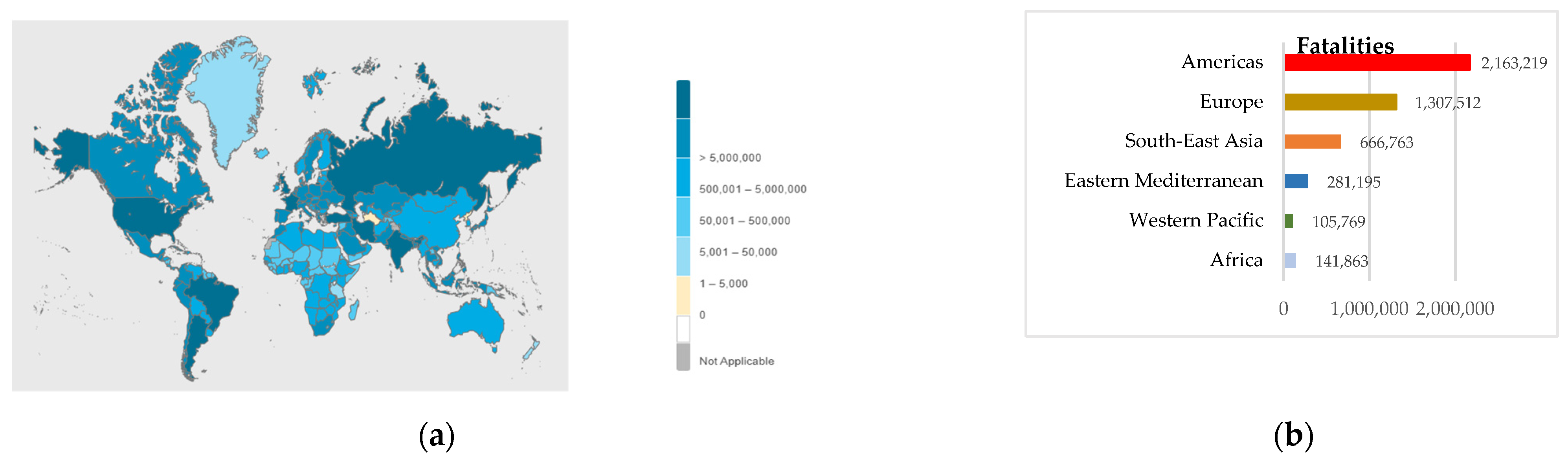
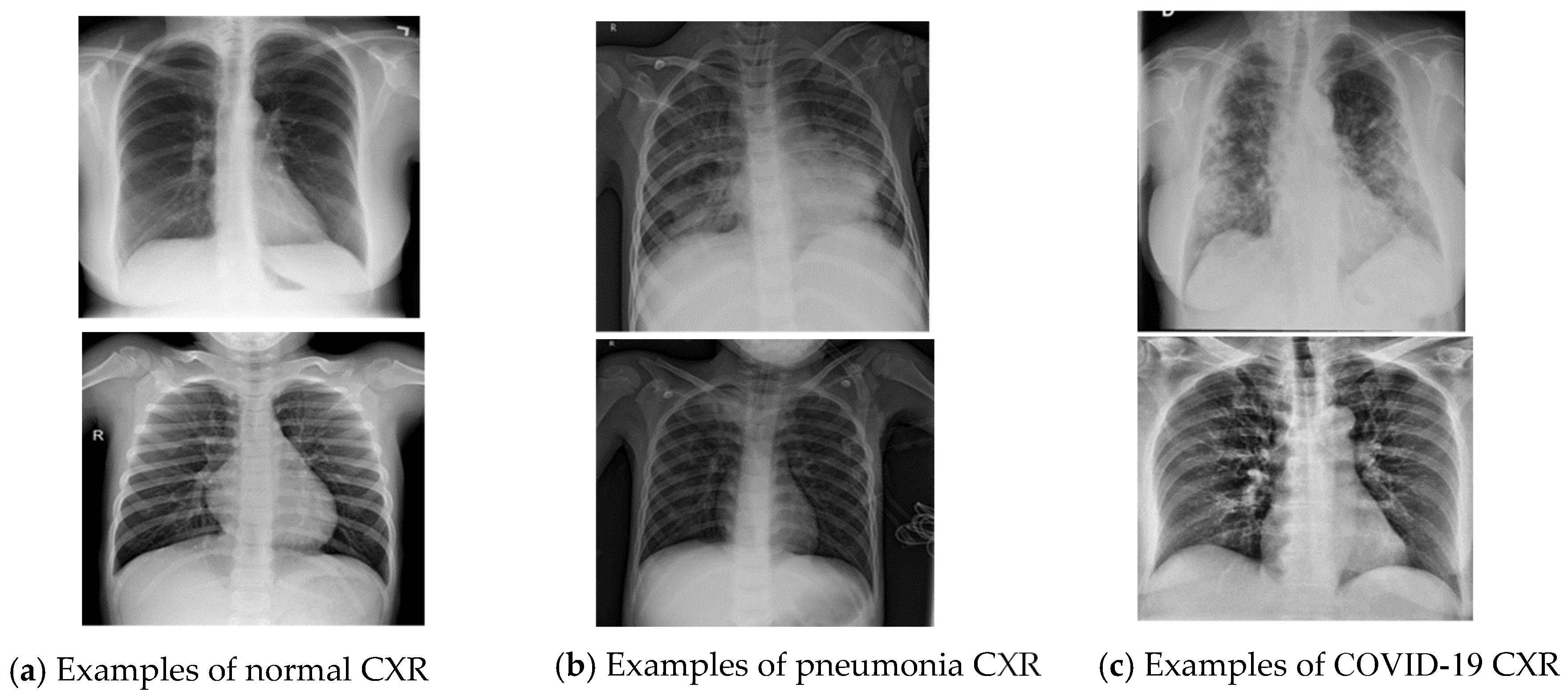
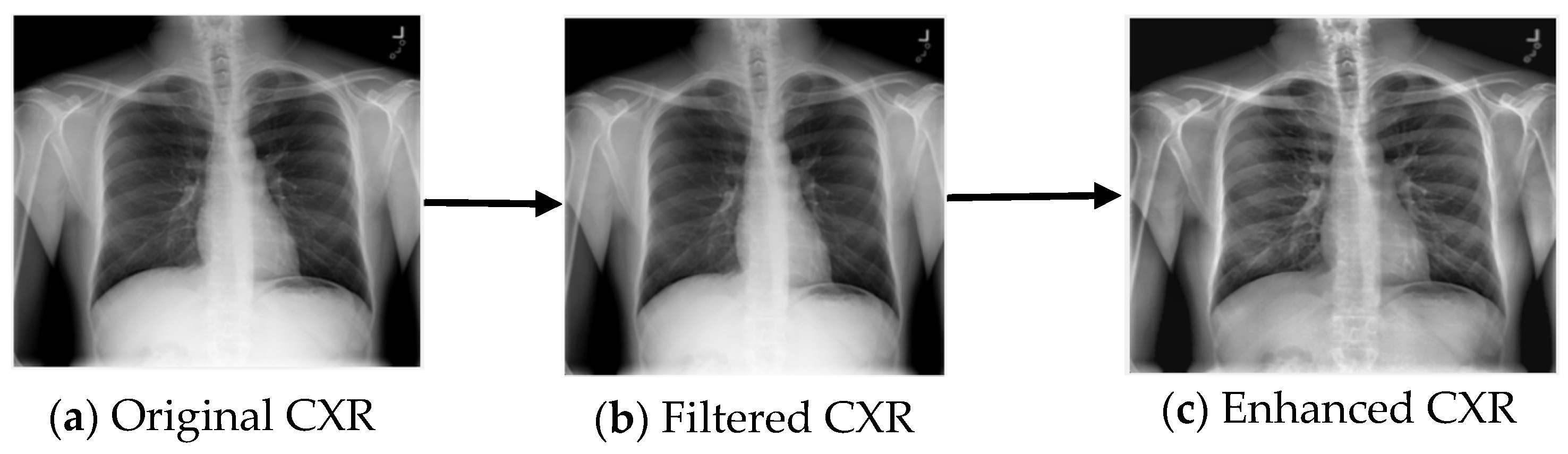
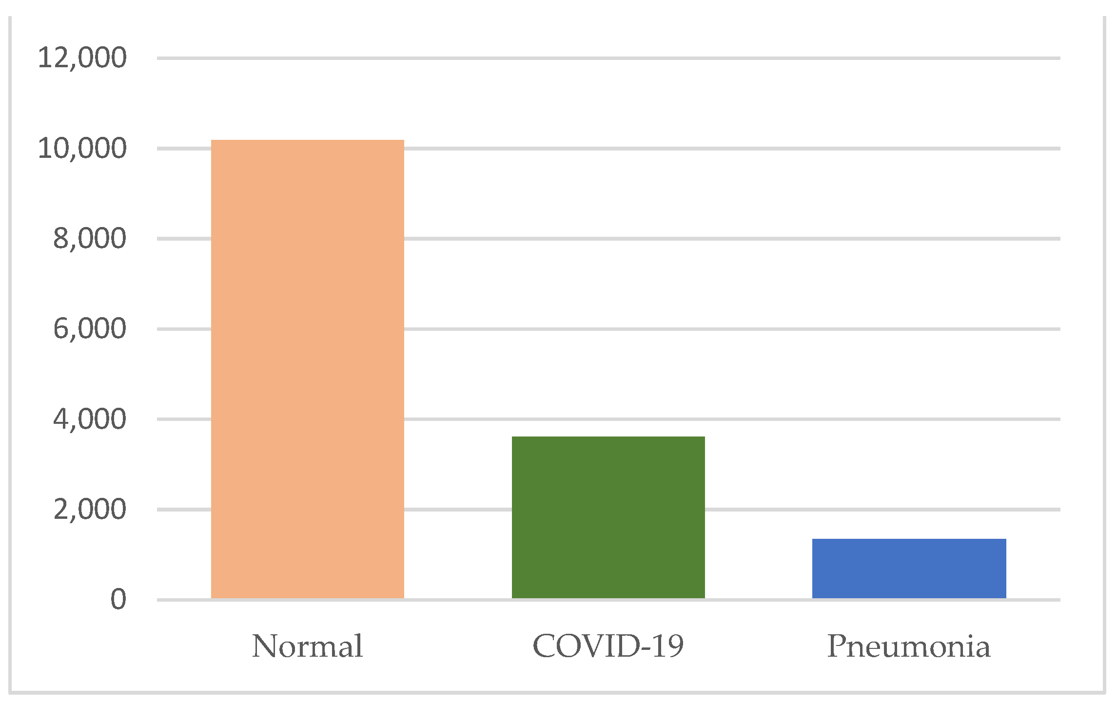
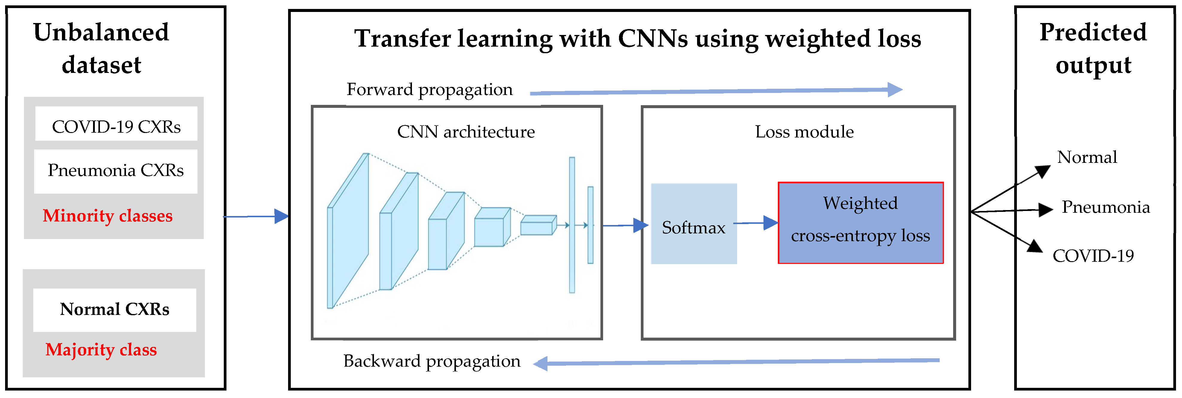
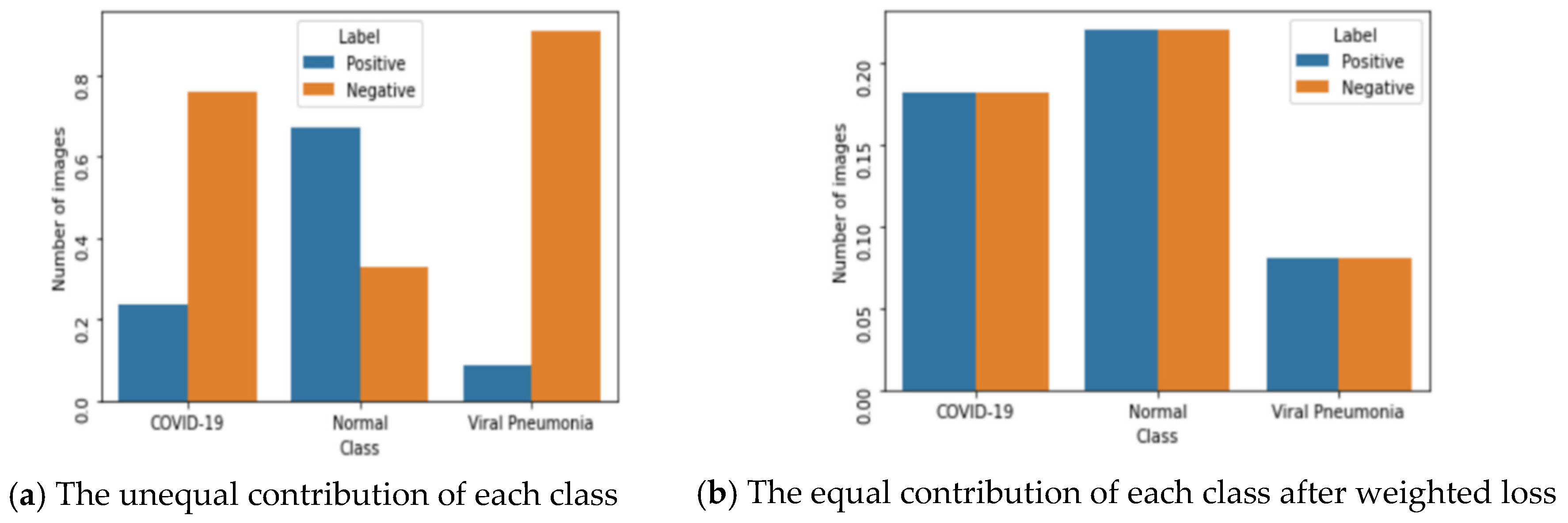
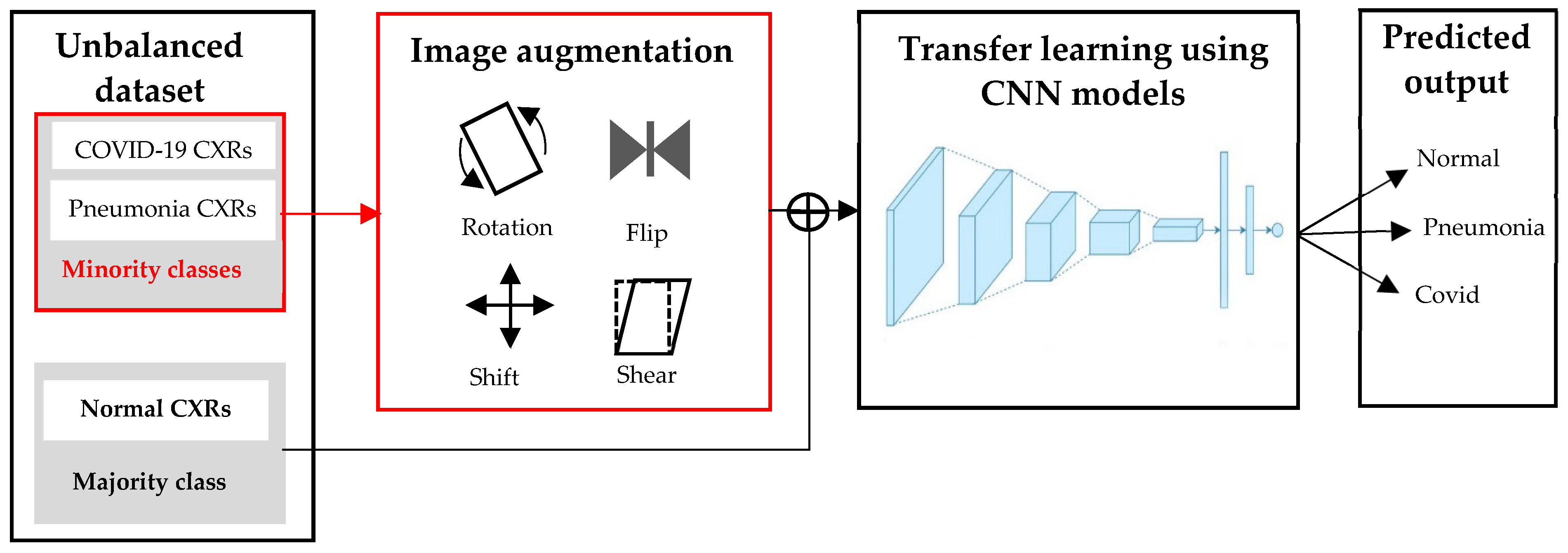
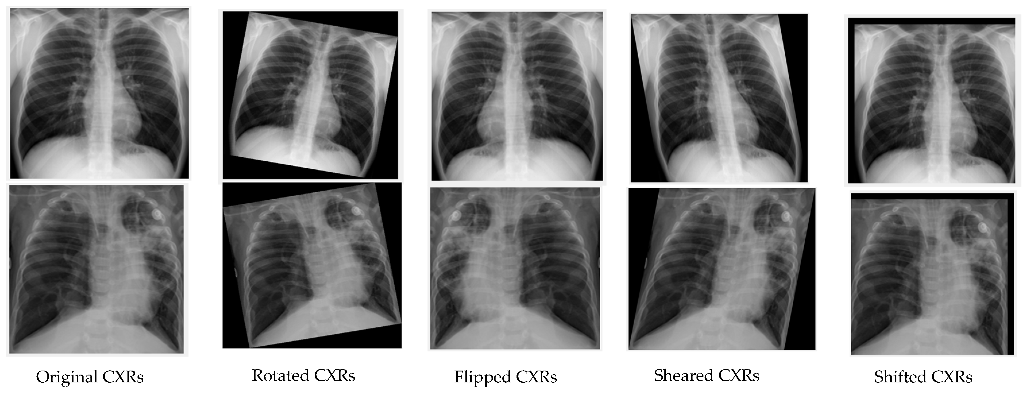
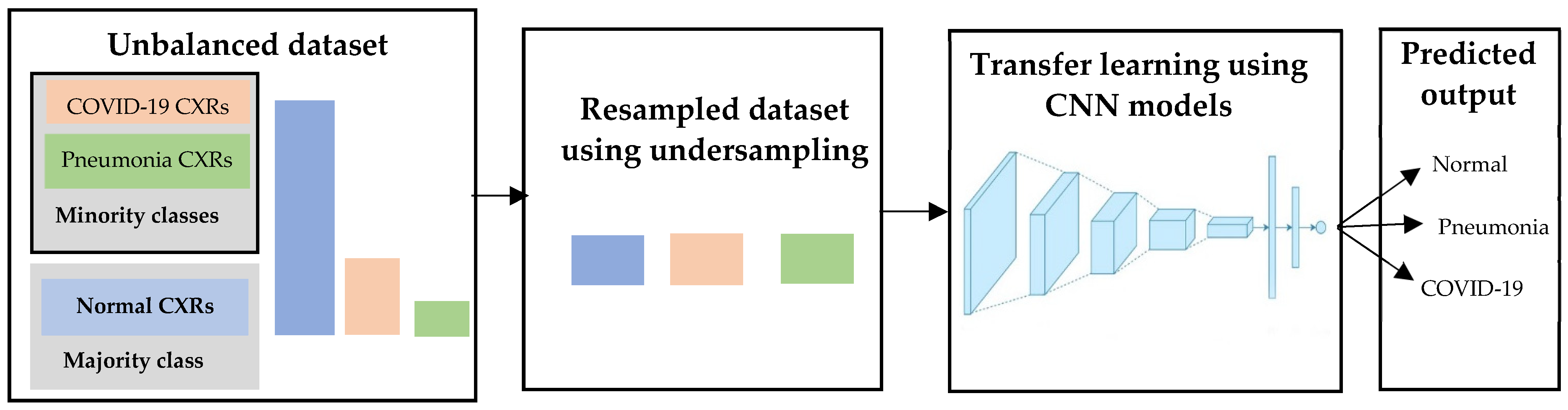
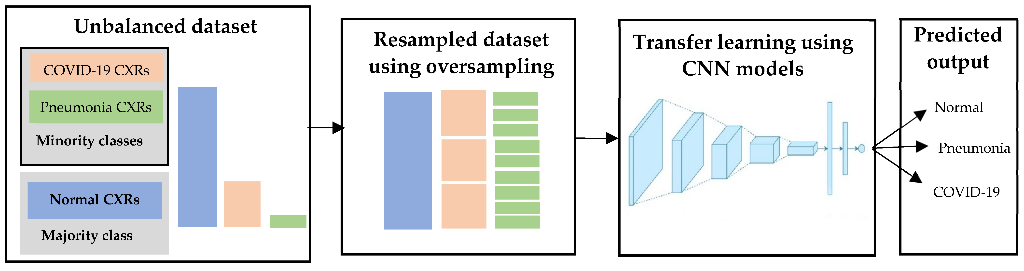
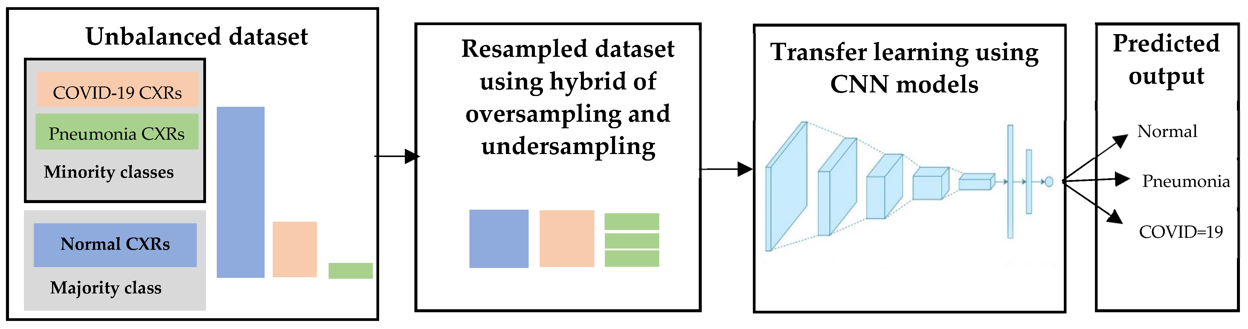
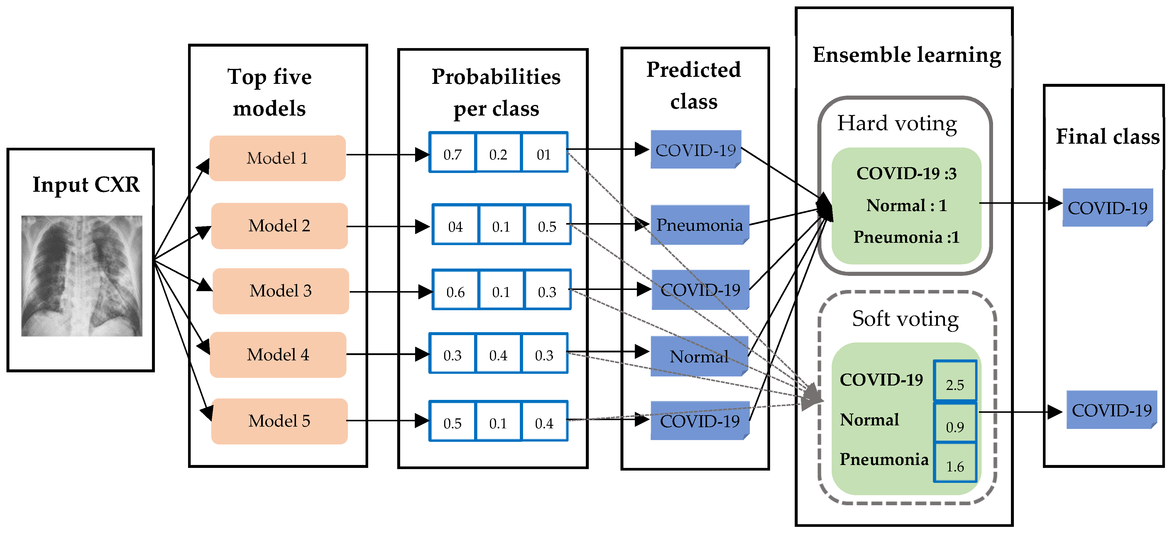
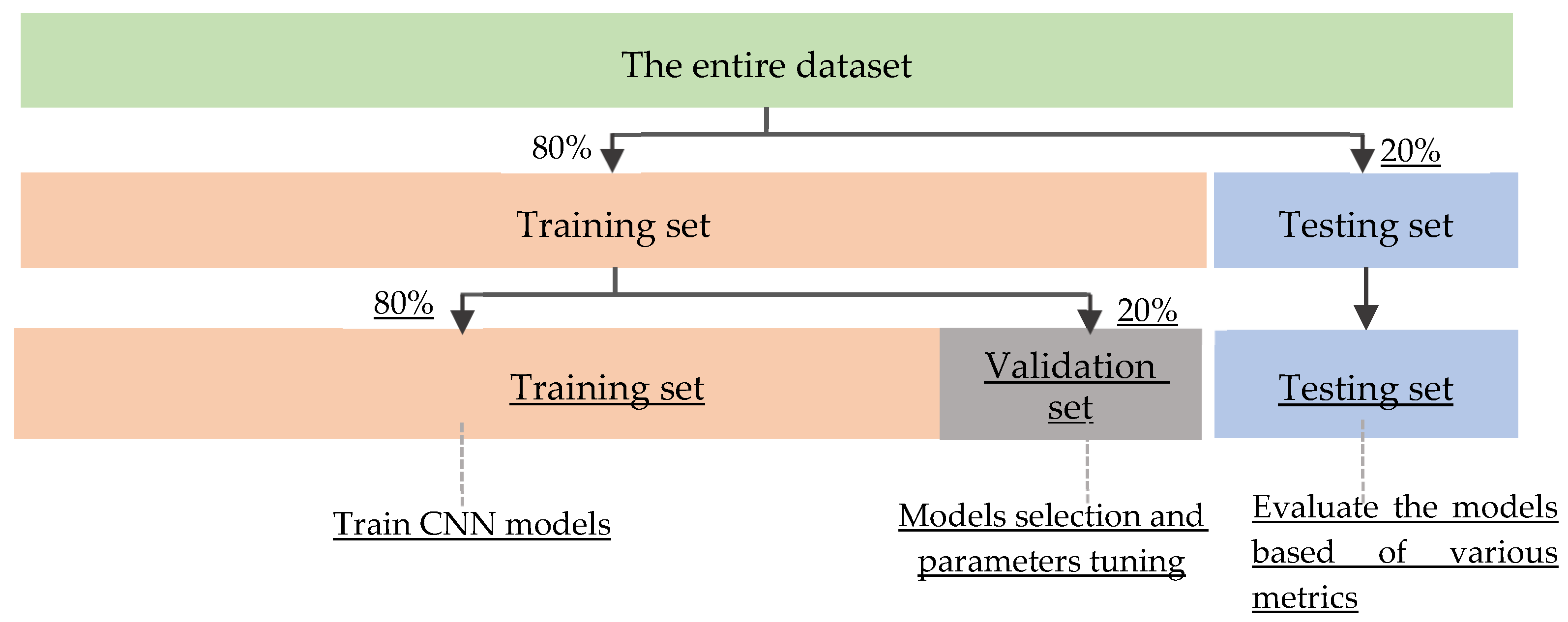
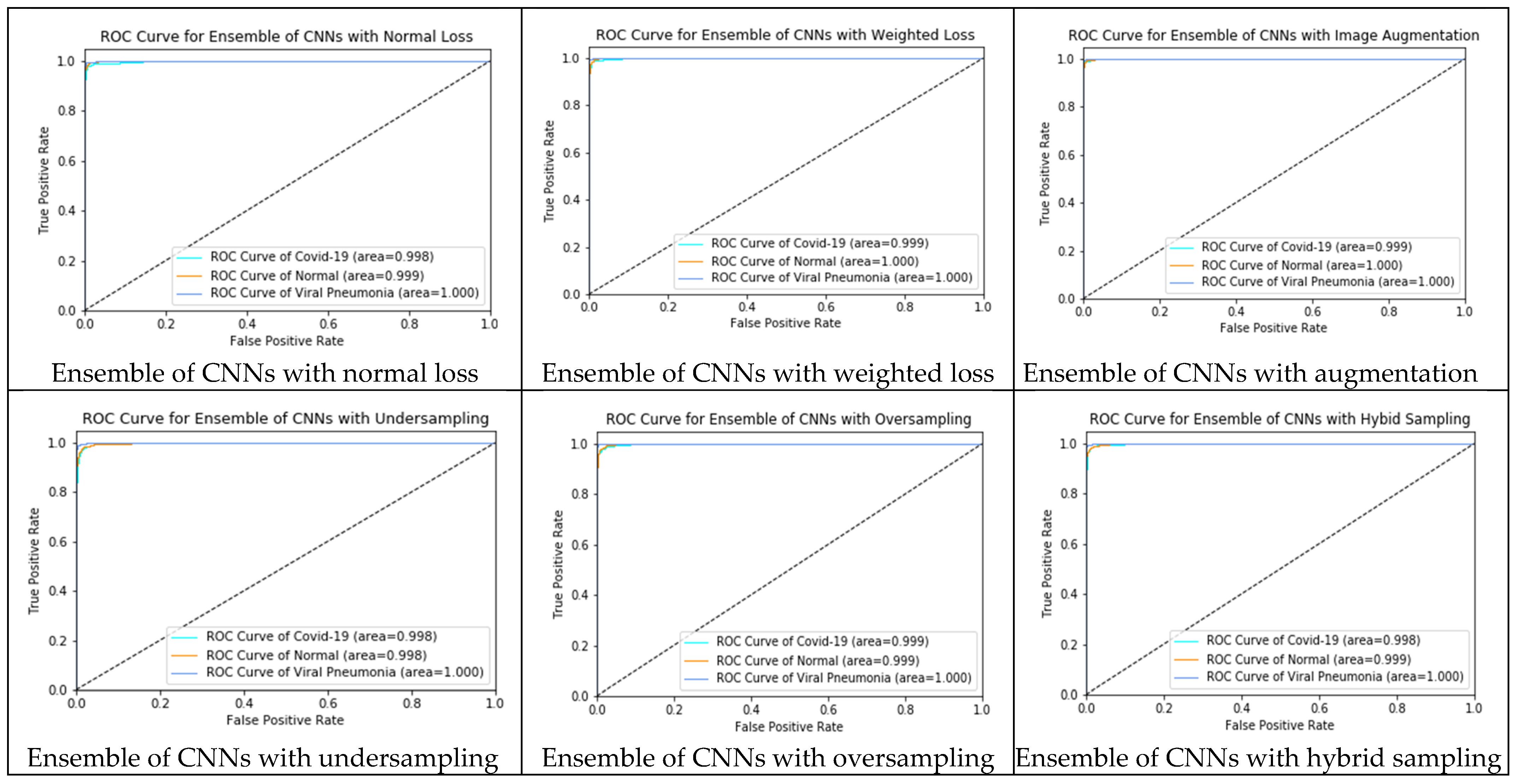
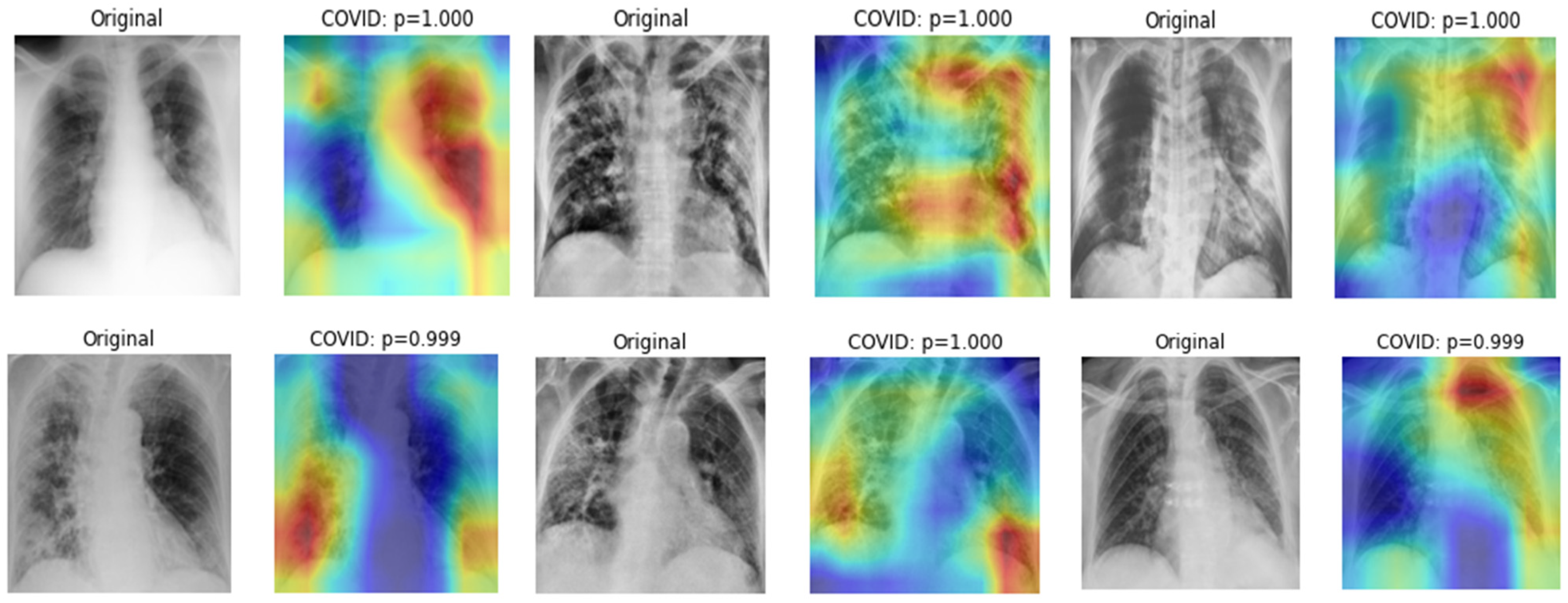
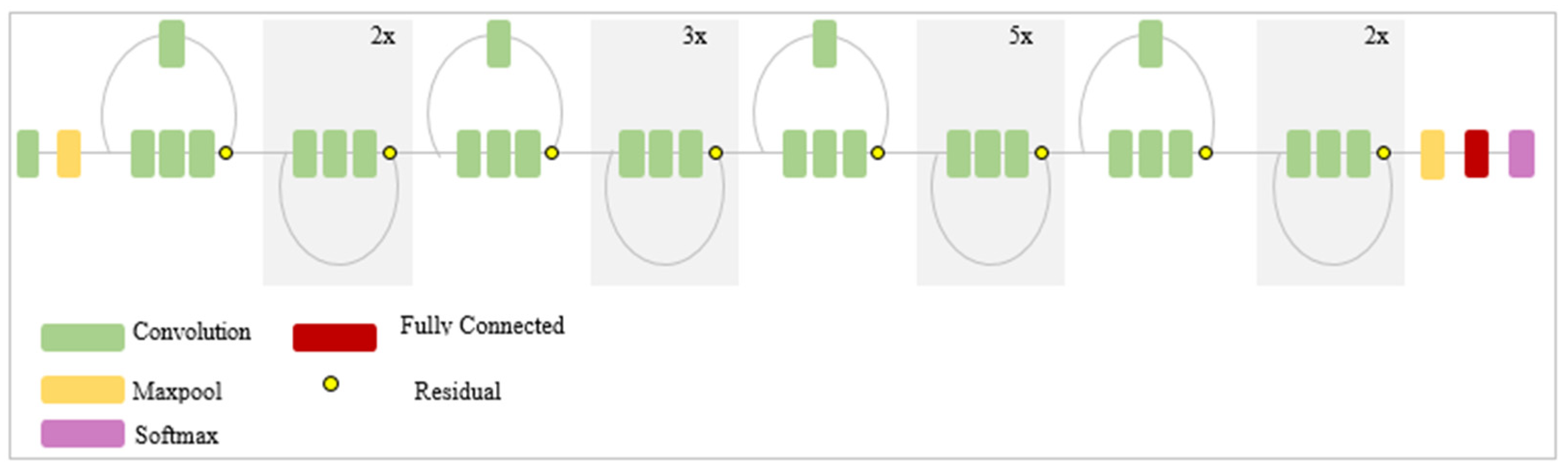
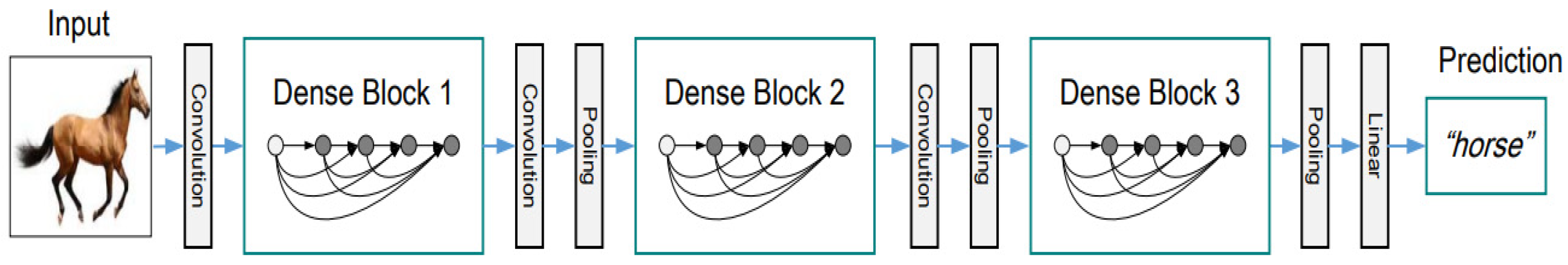
Figure 3.
Block diagram of the proposed study.

Figure 4.
Image preprocessing using median filter and CLAHE.

Figure 5.
Segmentation of lung regions using DeepLabV3+ and cropping.

Figure 6.
The unbalanced class distribution of the dataset.

Figure 7.
Transfer learning of CNNs with the weighted loss on the unbalanced dataset.

Figure 8.
The contribution of positive and negative labels within each class.

Figure 9.
Deep learning with image augmentation on the unbalanced dataset.

Figure 10.
Augmented CXRs using rotation, flipping, shearing, and shifting.

Figure 11.
Deep learning with undersampling on the unbalanced dataset. Normal and COVID-19 CXRs were randomly removed to ensure a better balance with the number of pneumonia CXRs.
Figure 11.
Deep learning with undersampling on the unbalanced dataset. Normal and COVID-19 CXRs were randomly removed to ensure a better balance with the number of pneumonia CXRs.

Figure 12.
Deep learning with oversampling on the unbalanced dataset. COVID-19 and pneumonia CXRs were randomly duplicated to ensure a better balance with the number of normal CXRs.
Figure 12.
Deep learning with oversampling on the unbalanced dataset. COVID-19 and pneumonia CXRs were randomly duplicated to ensure a better balance with the number of normal CXRs.

Figure 13.
Deep learning with hybrid resampling on an unbalanced dataset.

Figure 14.
Ensemble learning using majority hard voting and soft voting.

Figure 15.
Data partition and training of CNNs using holdout strategy.

Figure 16.
ROC curves (true positive rate vs. false positive rate) of each ensemble classifier.

Figure 17.
The indicative regions of COVID-19 biomarkers highlighted by DenseNet201.

Table 1.
COVID-19 RADIOGRAPHY DATABASE (version 2).
| Class | Number of Images | File Type | Image Resolution |
|---|---|---|---|
| Normal | 10,192 | PNG | 299 × 299 |
| COVID-19 | 3616 | PNG | 299 × 299 |
| Pneumonia | 1345 | PNG | 299 × 299 |
Table 2.
The data associated with each approach for handling unbalanced class, and hyperparameters for fine-tuning CNNs.
Table 2.
The data associated with each approach for handling unbalanced class, and hyperparameters for fine-tuning CNNs.
| Unbalanced Data Handling Approaches | Methods | Data | Hyperparameters of CNNs | ||||
|---|---|---|---|---|---|---|---|
| COVID-19 | Normal | Pneumonia | α | β_1 | β_2 | ||
| Approach 0 | Normal loss | 2893 | 8154 | 1076 | 0.001 | 0.9 | 0.999 |
| Approach 1 | Weighted loss | 2893 | 8154 | 1076 | 0.001 | 0.9 | 0.999 |
| Approach 2 | Image augmentation | 5393 | 4363 | 8154 | 0.001 | 0.9 | 0.999 |
| Approach 3 | Undersampling | 1013 | 1223 | 1076 | 0.001 | 0.9 | 0.999 |
| Approach 4 | Oversampling | 8100 | 8154 | 8070 | 0.001 | 0.9 | 0.999 |
| Approach 5 | Hybrid sampling | 2893 | 2854 | 2690 | 0.001 | 0.9 | 0.999 |
Table 3.
Classification results of normal, pneumonia, and COVID-19 on the whole CXRs using 11 CNNs (Approach 0 without lung segmentation: Unbalanced dataset).
Table 3.
Classification results of normal, pneumonia, and COVID-19 on the whole CXRs using 11 CNNs (Approach 0 without lung segmentation: Unbalanced dataset).
| Deep CNNs | Accuracy | Sensitivity | Specificity | AUC | F-Measure |
|---|---|---|---|---|---|
| XceptionNet | 97.07% | 97.13% | 92.77% | 99.80% | 96.20% |
| InceptionV3 | 95.10% | 98.57% | 93.63% | 99.57% | 91.60% |
| VGG-16 | 83.97% | 99.87% | 67.40% | 99.30% | 74.77% |
| VGG-19 | 87.60% | 97.27% | 79.87% | 97.80% | 82.80% |
| ResNet50 | 97.70% | 99.47% | 96.37% | 99.90% | 95.23% |
| ResNet152 | 95.83% | 97.27% | 91.53% | 99.53% | 93.40% |
| MobileNetV2 | 97.17% | 98.07% | 94.57% | 98.93% | 94.13% |
| DenseNet201 | 95.97% | 95.43% | 96.67% | 98.37% | 93.23% |
| InceptionResNetV2 | 96.53% | 98.67% | 94.53% | 99.70% | 93.97% |
| EfficientNetB7 | 88.43% | 89.37% | 91.50% | 98.23% | 83.80% |
| NasNetMobile | 97.97% | 98.97% | 96.03% | 99.90% | 94.90% |
Table 4.
Classification results of normal, pneumonia, and COVID-19 using the cropped lungs and 11 CNNs (Approach 0: Unbalanced dataset).
Table 4.
Classification results of normal, pneumonia, and COVID-19 using the cropped lungs and 11 CNNs (Approach 0: Unbalanced dataset).
| Deep CNNs | Accuracy | Sensitivity | Specificity | AUC | F-Measure |
|---|---|---|---|---|---|
| XceptionNet | 97.40% | 99.37% | 94.97% | 99.90% | 95.17% |
| InceptionV3 | 86.67% | 87.20% | 80.23% | 99.03% | 77.83% |
| VGG-16 | 83.90% | 99.33% | 74.07% | 98.60% | 72.77% |
| VGG-19 | 86.03% | 94.83% | 69.60% | 96.73% | 78.30% |
| ResNet50 | 86.63% | 98.83% | 76.53% | 98.87% | 83.57% |
| ResNet152 | 94.27% | 98.27% | 89.50% | 99.33% | 88.20% |
| MobileNetV2 | 97.23% | 98.33% | 95.43% | 99.67% | 94.63% |
| DenseNet201 | 95.47% | 99.40% | 89.63% | 99.67% | 93.63% |
| InceptionResNetV2 | 97.17% | 99.07% | 94.00% | 99.80% | 95.30% |
| EfficientNetB7 | 83.37% | 94.87% | 64.83% | 97.47% | 80.43% |
| NasNetMobile | 93.13% | 94.07% | 94.20% | 99.17% | 87.60% |
Table 5.
Classification results of normal, pneumonia and COVID-19 using cropped lungs and 11 CNNs with Weighted Loss (Approach 1).
Table 5.
Classification results of normal, pneumonia and COVID-19 using cropped lungs and 11 CNNs with Weighted Loss (Approach 1).
| Deep CNNs | Accuracy | Sensitivity | Specificity | AUC | F-Measure |
|---|---|---|---|---|---|
| XceptionNet | 98.17% | 98.33% | 98.53% | 99.93% | 97.07% |
| InceptionV3 | 93.50% | 95.13% | 95.23% | 99.67% | 88.47% |
| VGG-16 | 96.73% | 95.33% | 97.10% | 99.33% | 94.03% |
| VGG-19 | 91.60% | 85.50% | 88.70% | 98.07% | 83.90% |
| ResNet50 | 97.63% | 96.93% | 97.90% | 99.70% | 95.10% |
| ResNet152 | 97.40% | 96.03% | 97.53% | 99.47% | 95.33% |
| MobileNetV2 | 97.57% | 97.50% | 97.53% | 99.63% | 95.20% |
| DenseNet201 | 98.00% | 97.90% | 98.50% | 99.80% | 95.67% |
| InceptionResNetV2 | 96.63% | 95.53% | 96.10% | 99.30% | 94.17% |
| EfficientNetB7 | 97.13% | 98.10% | 97.70% | 99.87% | 92.10% |
| NasNetMobile | 95.93% | 97.13% | 92.47% | 99.77% | 93.30% |
Table 6.
Classification results of normal, pneumonia and COVID-19 using cropped lungs and 11 CNNs with Image Augmentation (Approach 2).
Table 6.
Classification results of normal, pneumonia and COVID-19 using cropped lungs and 11 CNNs with Image Augmentation (Approach 2).
| Deep CNNs | Accuracy | Sensitivity | Specificity | AUC | F-Measure |
|---|---|---|---|---|---|
| XceptionNet | 97.60% | 98.23% | 98.07% | 99.90% | 95.43% |
| InceptionV3 | 95.80% | 97.00% | 96.83% | 99.83% | 92.33% |
| VGG-16 | 95.17% | 95.90% | 96.53% | 99.50% | 92.23% |
| VGG-19 | 95.67% | 94.47% | 94.03% | 99.07% | 92.03% |
| ResNet50 | 97.13% | 97.40% | 97.57% | 99.70% | 94.97% |
| ResNet152 | 96.43% | 97.03% | 95.77% | 99.27% | 93.50% |
| MobileNetV2 | 98.43% | 98.20% | 98.23% | 99.83% | 96.20% |
| DenseNet201 | 98.57% | 98.17% | 97.40% | 99.87% | 97.70% |
| InceptionResNetV2 | 98.50% | 98.50% | 98.50% | 99.87% | 97.43% |
| EfficientNetB7 | 93.87% | 95.40% | 95.50% | 98.67% | 85.50% |
| NasNetMobile | 98.20% | 98.33% | 98.47% | 99.87% | 96.73% |
Table 7.
Classification results of normal and pneumonia and COVID-19 using cropped lungs and 11 CNNs with Undersampling (Approach 3).
Table 7.
Classification results of normal and pneumonia and COVID-19 using cropped lungs and 11 CNNs with Undersampling (Approach 3).
| Deep CNNs | Accuracy | Sensitivity | Specificity | AUC | F-Measure |
|---|---|---|---|---|---|
| XceptionNet | 97.80% | 97.93% | 97.87% | 99.77% | 96.075 |
| InceptionV3 | 96.63% | 93.13% | 94.13% | 99.37% | 93.93% |
| VGG-16 | 95.57% | 95.50% | 96.77% | 99.07% | 92.27% |
| VGG-19 | 94.67% | 93.77% | 95.37% | 98.70% | 90.60% |
| ResNet50 | 97.77% | 97.80% | 98.13% | 99.83% | 96.33% |
| ResNet152 | 96.67% | 96.67% | 97.60% | 99.60% | 93.43% |
| MobileNetV2 | 96.33% | 94.97% | 96.07% | 99.30% | 91.63% |
| DenseNet201 | 96.33% | 97.17% | 96.73% | 99.57% | 93.87% |
| InceptionResNetV2 | 96.77% | 96.67% | 97.17% | 98.50% | 94.73% |
| EfficientNetB7 | 97.57% | 95.67% | 96.20% | 99.57% | 95.83% |
| NasNetMobile | 97.40% | 95.47% | 97.17% | 99.50% | 95.50% |
Table 8.
Classification results of normal, pneumonia and COVID-19 using cropped lungs and 11 CNNs with Oversampling (Approach 4).
Table 8.
Classification results of normal, pneumonia and COVID-19 using cropped lungs and 11 CNNs with Oversampling (Approach 4).
| Deep CNNs | Accuracy | Sensitivity | Specificity | AUC | F-Measure |
|---|---|---|---|---|---|
| XceptionNet | 98.63% | 97.57% | 98.23% | 99.90% | 97.47% |
| InceptionV3 | 96.27% | 97.57% | 96.43% | 99.53% | 93.43% |
| VGG-16 | 96.27% | 96.20% | 96.83% | 99.37% | 93.73% |
| VGG-19 | 92.93% | 94.20% | 95.00% | 98.70% | 88.77% |
| ResNet50 | 97.77% | 97.27% | 97.70% | 99.63% | 96.17% |
| ResNet152 | 97.37% | 97.77% | 97.73% | 99.77% | 95.43% |
| MobileNetV2 | 97.90% | 96.10% | 97.40% | 99.77% | 95.83% |
| DenseNet201 | 98.20% | 98.07% | 97.23% | 99.77% | 97.27% |
| InceptionResNetV2 | 98.67% | 98.17% | 98.23% | 99.90% | 97.63% |
| EfficientNetB7 | 89.03% | 90.00% | 92.07% | 98.97% | 84.90% |
| NasNetMobile | 97.80% | 98.03% | 99.83% | 99.83% | 96.17% |
Table 9.
Classification results of normal, pneumonia and COVID-19 using the cropped lungs and 11 CNNs with Hybrid sampling (Approach 5).
Table 9.
Classification results of normal, pneumonia and COVID-19 using the cropped lungs and 11 CNNs with Hybrid sampling (Approach 5).
| Deep CNNs | Accuracy | Sensitivity | Specificity | AUC | F-Measure |
|---|---|---|---|---|---|
| XceptionNet | 97.36% | 97.86% | 97.70% | 99.63% | 95.80% |
| InceptionV3 | 93.23% | 95.86% | 94.70% | 99.60% | 86.40% |
| VGG-16 | 95.93% | 95.23% | 96.37% | 99.03% | 92.43% |
| VGG-19 | 95.97% | 96.13% | 96.63% | 99.30% | 93.30% |
| ResNet50 | 93.63% | 94.30% | 94.67% | 99.00% | 90.90% |
| ResNet152 | 93.60% | 90.37% | 91.70% | 94.90% | 89.50% |
| MobileNetV2 | 97.23% | 98.33% | 95.43% | 99.67% | 94.63% |
| DenseNet201 | 95.80% | 96.43% | 97.07% | 99.70% | 93.73% |
| InceptionResNetV2 | 92.23% | 92.40% | 93.83% | 96.47% | 83.73% |
| EfficientNetB7 | 93.03% | 92.93% | 94.83% | 99.67% | 88.50% |
| NasNetMobile | 96.67% | 97.40% | 97.43% | 99.77% | 94.63% |
Table 10.
Ensemble of top five models from each approach using majority soft voting and hard voting.
Table 10.
Ensemble of top five models from each approach using majority soft voting and hard voting.
| Deep CNNs | Voting Strategy | Accuracy | Sensitivity | Specificity | AUC | F-Measure |
|---|---|---|---|---|---|---|
| Ensemble of Approach 0 | Soft Voting | 97.93% | 98.43% | 98.40% | 99.90% | 96.70% |
| Hard Voting | 96.63% | 97.97% | 98.44% | N/A | 96.62% | |
| Ensemble of Approach 1 | Soft Voting | 99.03% | 98.97% | 99.20% | 99.97% | 98.23% |
| Hard Voting | 98.35% | 98.66% | 99.11% | N/A | 97.88% | |
| Ensemble of Approach 2 | Soft Voting | 99.23% | 99.27% | 99.27% | 99.97% | 98.30% |
| Hard Voting | 98.84% | 99.05% | 99.38% | N/A | 98.41% | |
| Ensemble of Approach 3 | Soft Voting | 98.00% | 98.17% | 98.37% | 99.87% | 96.53% |
| Hard Voting | 96.53% | 97.63% | 98.33% | N/A | 96.13% | |
| Ensemble of Approach 4 | Soft Voting | 99.17% | 98.87% | 98.80% | 99.93% | 98.57% |
| Hard Voting | 98.61% | 98.28% | 98.90% | N/A | 98.43% | |
| Ensemble of Approach 5 | Soft Voting | 98.00% | 99.33% | 95.93% | 99.90% | 96.63% |
| Hard Voting | 98.75% | 98.41% | 99.07% | N/A | 98.59% |
Table 11.
False-negative of COVID-19 (misclassification of COVID-19 CXRs as normal and pneumonia).
| Methods | False-Negative of COVID-19 |
|---|---|
| Ensemble of CNNs with normal loss | 14 |
| Ensemble of CNNs with weighted loss | 8 |
| Ensemble of CNNs with image augmentation | 8 |
| Ensemble of CNNs with undersampling | 7 |
| Ensemble of CNNs with oversampling | 9 |
| Ensemble of CNNs with hybrid sampling | 3 |
Table 12.
Previous studies vs. our proposed study.
| Authors | Classification Methods | Classification Strategy | Data | Performance |
|---|---|---|---|---|
| Hemdan et al. [10] | COVIDX-Net using six CNNs | Binary classification of normal and COVID-19 | COVID-19: 25 Normal: 25 | F-Measure 81% (normal) 91% (COVID-19) |
| Sahlol et al. [11] | Hybrid of InceptionNet as a feature extractor and Marine Predator as a feature selection method | Binary classification between COVID-19 and Normal | COVID-19: 200 Normal: 1675 | Accuracy 98.7% |
| COVID-19: 219 Normal: 1341 | Accuracy 99.6% | |||
| Alazab et al. [12] | VGG-16 based classification with and without data augmentation | Binary classification of healthy and COVID-19 | COVID-19: 70 Healthy: 28 (original dataset) | F-measure 95% |
| COVID-19: 500 Healthy: 500 (augmented) | F-measure 99% | |||
| Duran-Lopez et al. [13] | A customized deep learning model | Binary classification of non-findings and COVID-19 | COVID-19: 2589 Normal: 4337 | Accuracy 94.43% |
| Khasawneh et al. [14] | 2D CNN, VGG16, Mobile Nets | Binary classification of normal and COVID-19 | COVID-19: 1210 Normal: 1583 | Accuracy 98.7% |
| Wang et al. [15] | A custom deep learning algorithm | Multi-classification of normal, COVID-19 and pneumonia | COVID-19: 266 Normal: 8066 Pneumonia: 5526 | Sensitivity 80% |
| Brunese et al. [16] | VGG16 based transfer learning | Two staged binary classification:
| (i) Healthy: 3520 lung diseases: 3003 | Accuracy 96% |
| (ii) COVID-19: 250 lung diseases: 2753 | Accuracy 98% | |||
| Ahmed et al. [17] | A custom deep learning model with multiple feature extraction layers | Multi-classification of normal, COVID-19 and pneumonia | COVID-19: 238 Normal: 8851 Pneumonia: 6045 | Accuracy 97.48% |
| Yoo et al. [18] | Dee learning based decision tree classifier | Step by step binary classification:
| Normal: 558 Abnormal: 558 | Accuracy 98% |
| TB: 492 non TB: 492 | Accuracy 80% | |||
| COVID-19: 142 TB: 142 | Accuracy 95% | |||
| Ozturk et al. [19] | Modified Darknet-19 model | Binary classification of non-findings and COVID-19 | COVID-19: 125 Normal: 500 | Accuracy 98.08% |
| Multi classification of normal, COVID-19 and pneumonia | COVID-19: 125 Normal: 500 Pneumonia: 500 | Accuracy 87.02% | ||
| Ben Jabra et al. [20] | 16 state-of-the-art CNNs model and ensemble of those models using voting | Multi-classification of normal, COVID-19, and pneumonia | COVID-19: 237 Normal: 1338 Pneumonia: 1336 | Accuracy 99.31 % |
| Shelke et al. [21] | VGG-19, DenseNet-161 and ResNet-18 | Three-staged classification
| Normal: 526 Pneumonia: 605 TB: 382 | Accuracy 95.9% |
| COVID-19: 735 Pneumonia: 650 | Accuracy 98.9% | |||
| Mild: 80 Medium: 80 Severe: 80 | Accuracy 76% | |||
| Oh et al. [22] | A patch-based ResNet18 model | Multi-classification of normal, COVID-19, pneumonia and TB | COVID-19: 180 Normal: 191 Pneumonia: 74 TB: 57 | Sensitivity 92.5% |
| Rajaraman et al. [23] | Ensemble of iteratively pruned deep learning models | Multi-classification of normal, COVID-19 and pneumonia | COVID-19: 313 Normal: 7595 Pneumonia: 8792 | Accuracy 99.01% |
| Bridge et al. [24] | InceptionNet with GEV activation function | Binary classification of non-findings and COVID-19 | COVID-19: 129 Normal: 62,267 Pneumonia: 5689 | AUC 82% |
| Multi classification of normal, pneumonia and COVID-19 | AUC 73.1% | |||
| Nishio et al. [25] | Transfer learning of VGG-16 with a combination of data augmentation methods | Multi-classification of healthy, COVID-19 pneumonia, and non-COVID-19 pneumonia | COVID-19: 215 Healthy: 500 Pneumonia: 533 | Accuracy 83.6% |
| Our proposed study |
| Multi-classification of normal, COVID-19, and pneumonia | COVID-19: 3616 Normal: 10,192 Pneumonia: 1345 | Accuracy 99.23% Sensitivity 99.27% AUC 99.97 F-measure 98.3 |
Publisher’s Note: MDPI stays neutral with regard to jurisdictional claims in published maps and institutional affiliations. |
© 2021 by the authors. Licensee MDPI, Basel, Switzerland. This article is an open access article distributed under the terms and conditions of the Creative Commons Attribution (CC BY) license (https://creativecommons.org/licenses/by/4.0/).
Share and Cite
MDPI and ACS Style
Win, K.Y.; Maneerat, N.; Sreng, S.; Hamamoto, K. Ensemble Deep Learning for the Detection of COVID-19 in Unbalanced Chest X-ray Dataset. Appl. Sci. 2021, 11, 10528. https://doi.org/10.3390/app112210528
AMA Style
Win KY, Maneerat N, Sreng S, Hamamoto K. Ensemble Deep Learning for the Detection of COVID-19 in Unbalanced Chest X-ray Dataset. Applied Sciences. 2021; 11(22):10528. https://doi.org/10.3390/app112210528
Chicago/Turabian StyleWin, Khin Yadanar, Noppadol Maneerat, Syna Sreng, and Kazuhiko Hamamoto. 2021. "Ensemble Deep Learning for the Detection of COVID-19 in Unbalanced Chest X-ray Dataset" Applied Sciences 11, no. 22: 10528. https://doi.org/10.3390/app112210528
Note that from the first issue of 2016, this journal uses article numbers instead of page numbers. See further details here.