


Influence of the Demographic, Social, and Environmental Factors on the COVID-19 Pandemic—Analysis of the Local Variations Using Geographically Weighted Regression

Abstract
:1. Introduction
2. Materials and Methods
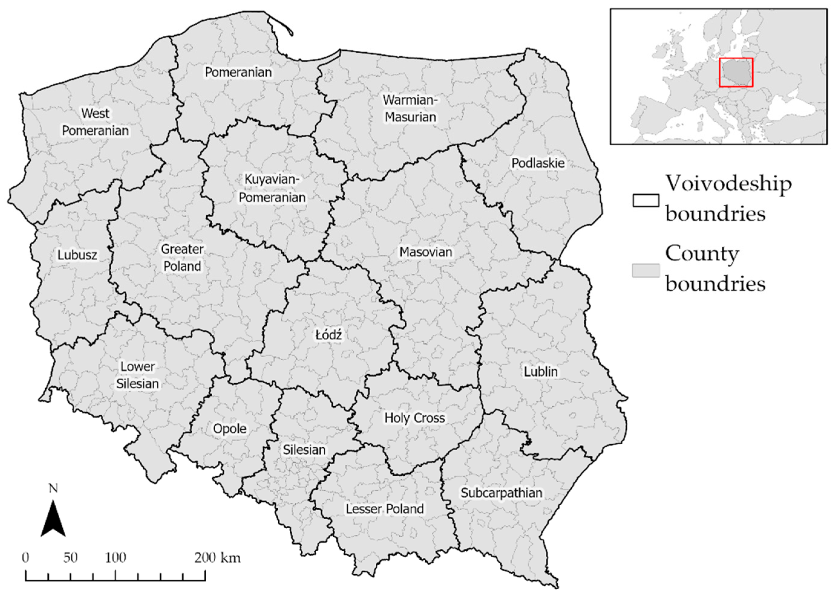
2.1. Study Area
2.2. Data Source and Processing
2.3. Research Method
- —dependent variable at location i
- —explanatory variable at location i
- —coordinate for location i
- —intercept location i
- —coefficient for explanatory variable k at location i
- —residual location i
3. Results
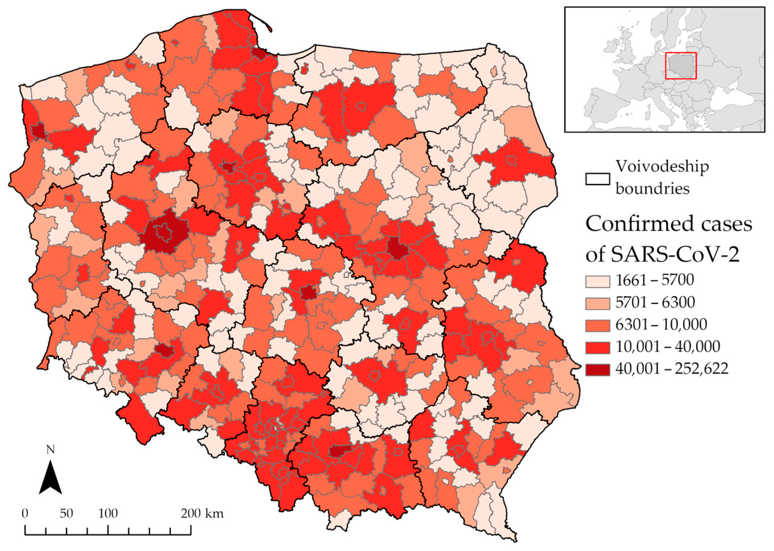
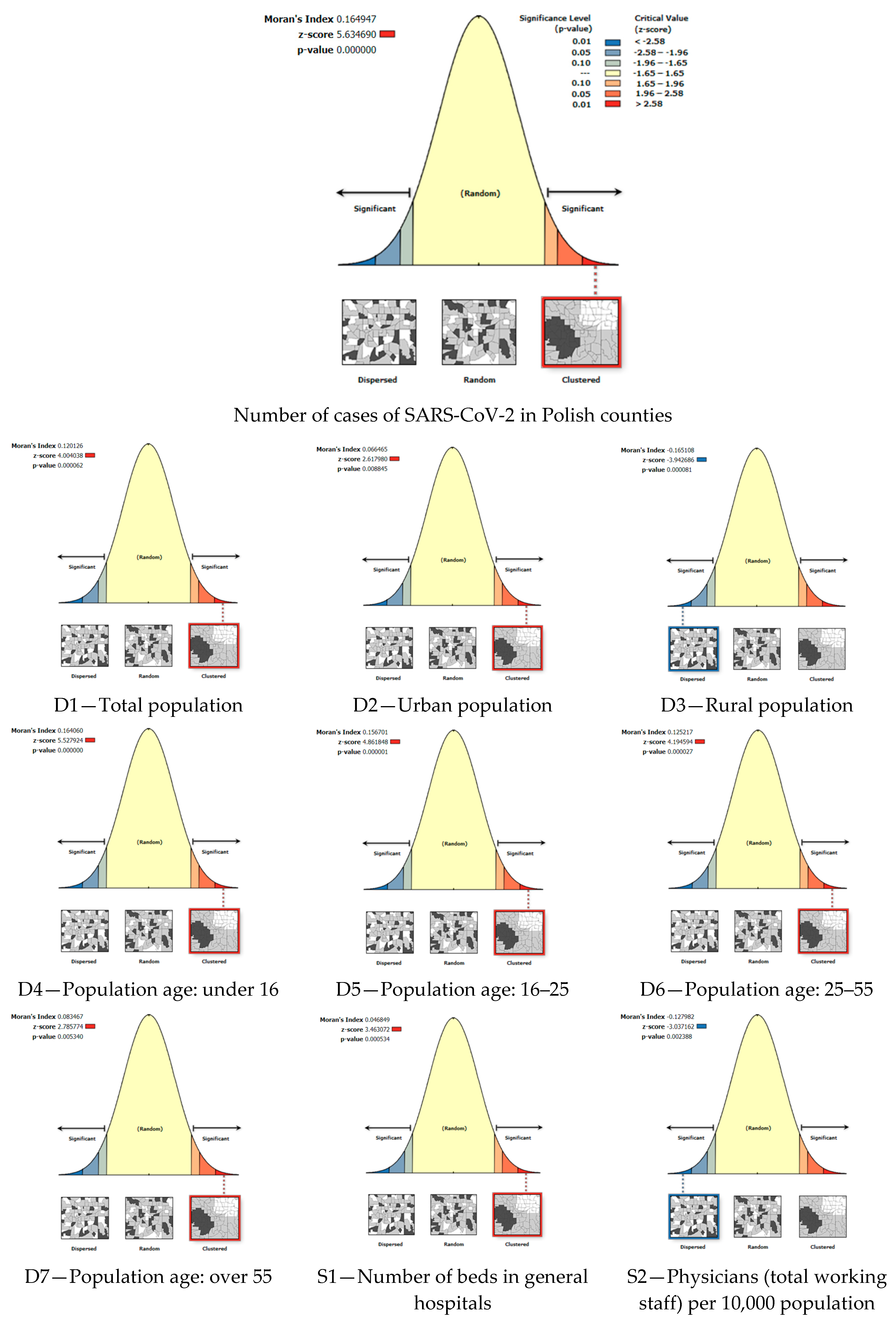
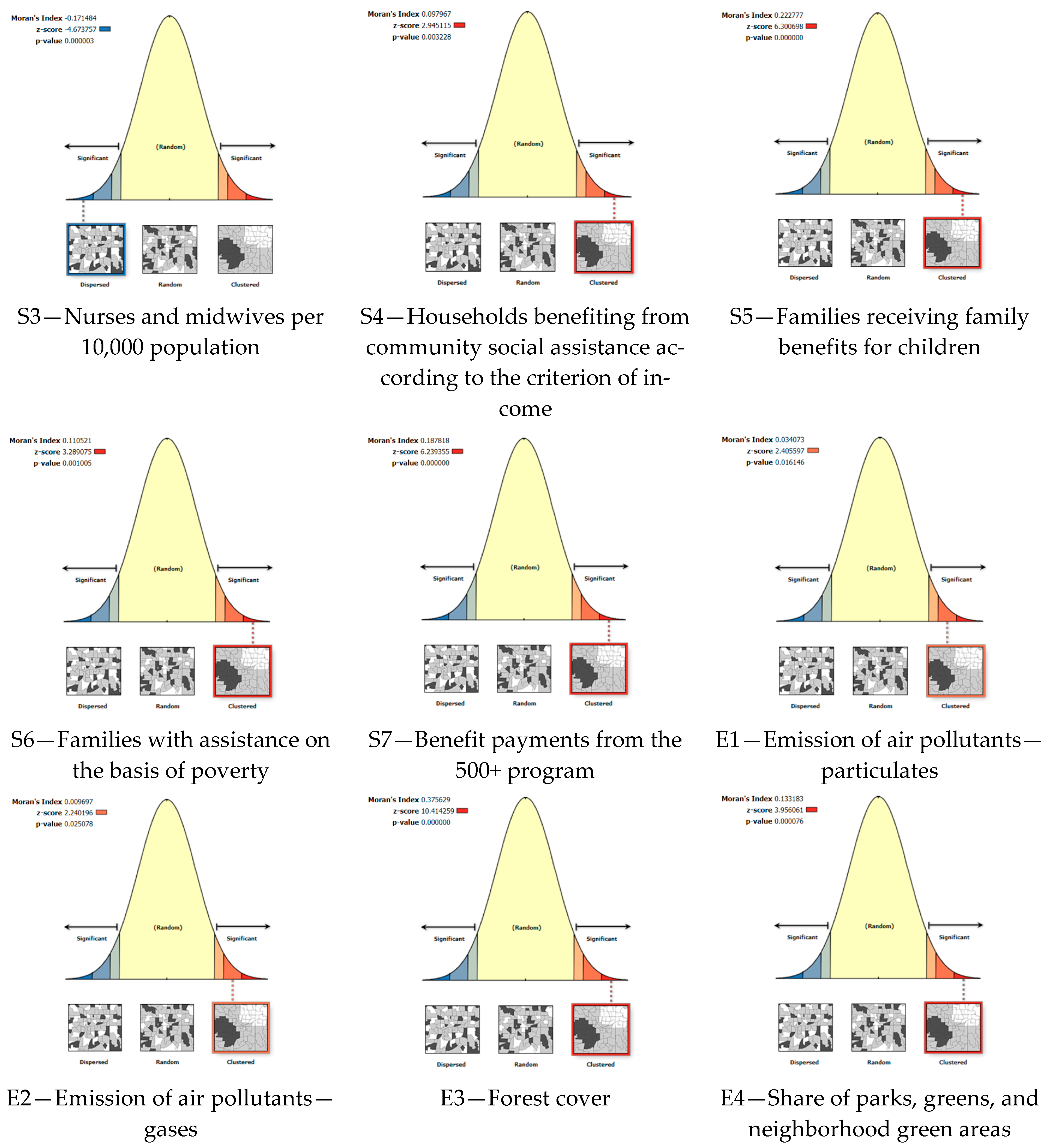
3.1. Spatial Autocorrelation Analysis
3.2. Influence of the Selected Variables on the Number of Cases of SARS-CoV-2
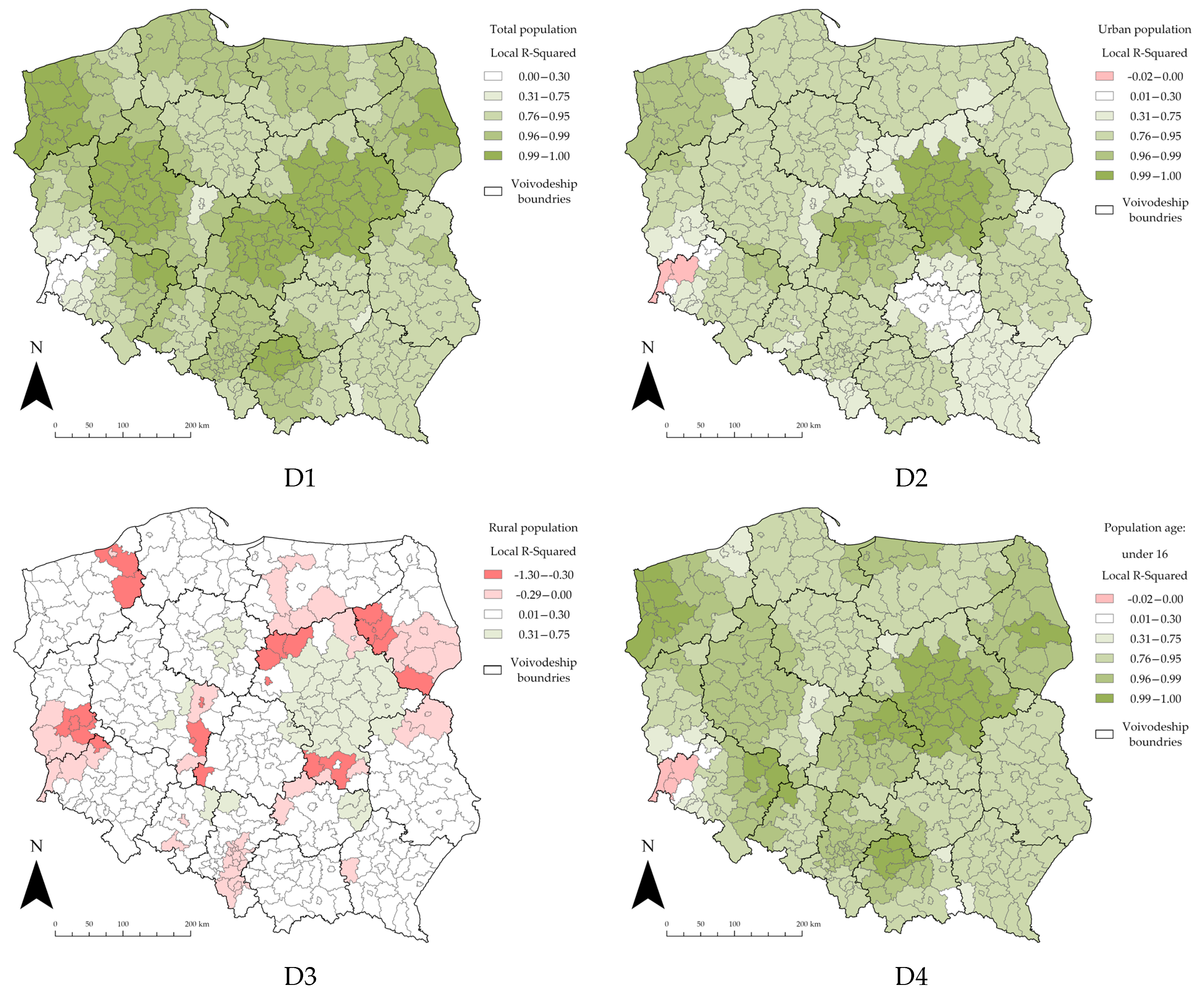
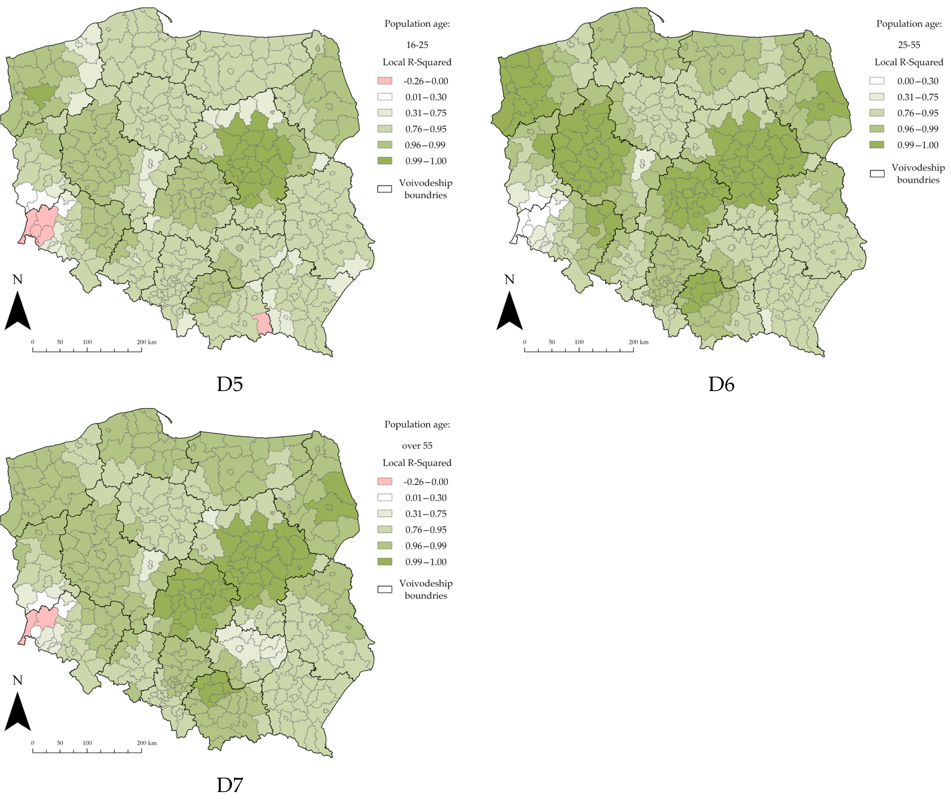
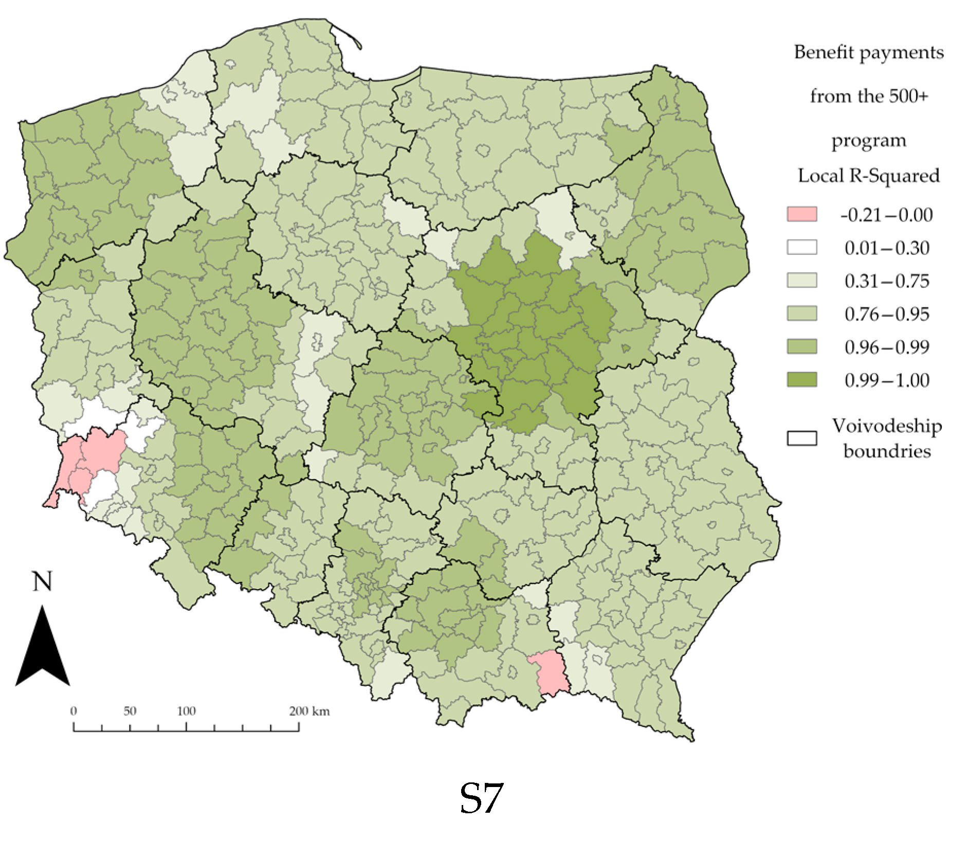
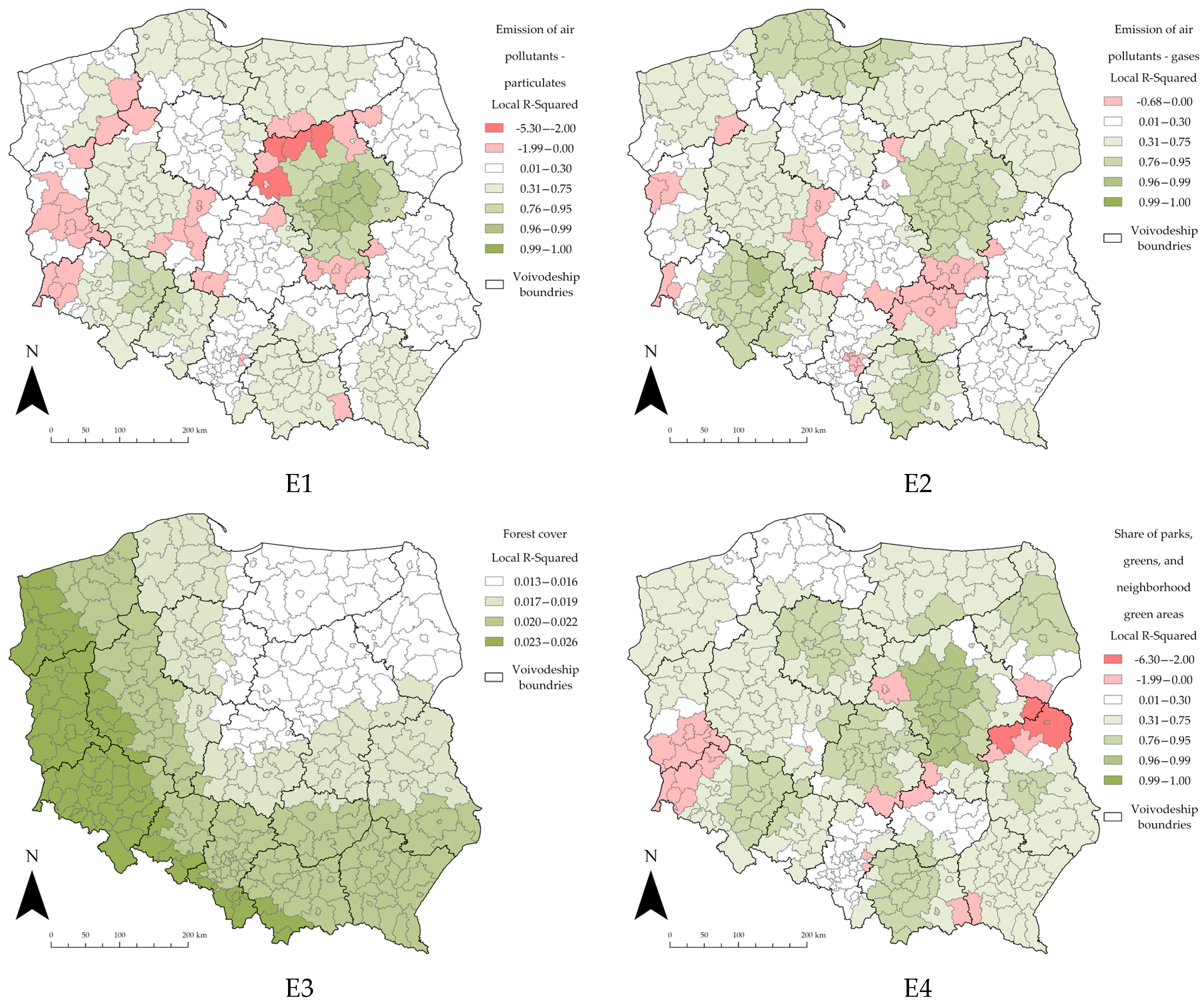
3.3. Local R2 Estimates
3.4. Residual Spatial Autocorrelation
4. Discussion
5. Conclusions
Supplementary Materials
Author Contributions
Funding
Institutional Review Board Statement
Conflicts of Interest
References
- Li, Q.; Guan, X.; Wu, P.; Wang, X.; Zhou, L.; Tong, Y.; Ren, R.; Leung, K.S.M.; Lau, E.H.Y.; Wong, J.Y.; et al. Early Transmission Dynamics in Wuhan, China, of Novel Coronavirus-Infected Pneumonia. N. Engl. J. Med. 2020, 382, 1199–1207. [Google Scholar] [CrossRef] [PubMed]
- Zhu, N.; Zhang, D.; Wang, W.; Li, X.; Yang, B.; Song, J.; Zhao, X.; Huang, B.; Shi, W.; Lu, R.; et al. A Novel Coronavirus from Patients with Pneumonia in China, 2019. N. Engl. J. Med. 2020, 382, 727–733. [Google Scholar] [CrossRef] [PubMed]
- Di Gennaro, F.; Pizzol, D.; Marotta, C.; Antunes, M.; Racalbuto, V.; Veronese, N.; Smith, L. Coronavirus diseases (COVID-19) current status and future perspectives: A narrative review. Int. J. Environ. Res. Public Health 2020, 17, 2690. [Google Scholar] [CrossRef] [PubMed]
- Wang, C.; Pan, R.; Wan, X.; Tan, Y.; Xu, L.; Ho, C.S.; Ho, R.C. Immediate psychological responses and associated factors during the initial stage of the 2019 coronavirus disease (COVID-19) epidemic among the general population in China. Int. J. Environ. Res. Public Health 2020, 17, 1729. [Google Scholar] [CrossRef] [PubMed]
- Linton, N.M.; Kobayashi, T.; Yang, Y.; Hayashi, K.; Akhmetzhanov, A.R.; Jung, S.M.; Yuan, B.; Kinoshita, R.; Nishiura, H. Incubation period and other epidemiological characteristics of 2019 novel coronavirus infections with right truncation: A statistical analysis of publicly available case data. J. Clin. Med. 2020, 9, 538. [Google Scholar] [CrossRef] [PubMed]
- Zhang, Y.; Ma, Z.F. Impact of the COVID-19 pandemic on mental health and quality of life among local residents in Liaoning Province, China: A cross-sectional study. Int. J. Environ. Res. Public Health 2020, 17, 2381. [Google Scholar] [CrossRef]
- Shekhar, R.; Sheikh, A.B.; Upadhyay, S.; Singh, M.; Kottewar, S.; Mir, H.; Barrett, E.; Pal, S. COVID-19 vaccine acceptance among health care workers in the united states. Vaccines 2021, 9, 119. [Google Scholar] [CrossRef] [PubMed]
- Zhang, Y.; Zhang, H.; Ma, X.; Di, Q. Mental health problems during the COVID-19 pandemics and the mitigation effects of exercise: A longitudinal study of college students in China. Int. J. Environ. Res. Public Health 2020, 17, 3722. [Google Scholar] [CrossRef]
- Marom, P.; Zalcman, B.G.; Dankner, R. Association between Self-Classification of COVID-19 Risk Levels and Adverse Lifestyle Changes among Physically Active Older Adults Following the Coronavirus Outbreak. Int. J. Environ. Res. Public Health 2022, 19, 7039. [Google Scholar] [CrossRef]
- Solomou, I.; Constantinidou, F. Prevalence and predictors of anxiety and depression symptoms during the COVID-19 pandemic and compliance with precautionary measures: Age and sex matter. Int. J. Environ. Res. Public Health 2020, 17, 4924. [Google Scholar] [CrossRef]
- Clemente-Suárez, V.J.; Navarro-Jiménez, E.; Jimenez, M.; Hormeño-Holgado, A.; Martinez-Gonzalez, M.B.; Benitez-Agudelo, J.C.; Perez-Palencia, N.; Laborde-Cárdenas, C.C.; Tornero-Aguilera, J.F. Impact of COVID-19 pandemic in public mental health: An extensive narrative review. Sustainability 2021, 13, 3221. [Google Scholar] [CrossRef]
- Meyer, J.; McDowell, C.; Lansing, J.; Brower, C.; Smith, L.; Tully, M.; Herring, M. Changes in physical activity and sedentary behavior in response to COVID-19 and their associations with mental health in 3052 us adults. Int. J. Environ. Res. Public Health 2020, 17, 6469. [Google Scholar] [CrossRef]
- Jin, Y.; Yang, H.; Ji, W.; Wu, W.; Chen, S.; Zhang, W.; Duan, G. Virology, epidemiology, pathogenesis, and control of COVID-19. Viruses 2020, 12, 372. [Google Scholar] [CrossRef] [PubMed]
- Lorent, D.; Nowak, R.; Roxo, C.; Lenartowicz, E.; Makarewicz, A.; Zaremba, B.; Nowak, S.; Kuszel, L.; Stefaniak, J.; Kierzek, R.; et al. Prevalence of Anti-SARS-CoV-2 Antibodies in Poznań, Poland, after the First Wave of the COVID-19 Pandemic. Vaccines 2021, 9, 541. [Google Scholar] [CrossRef] [PubMed]
- Sallam, M. COVID-19 vaccine hesitancy worldwide: A concise systematic review of vaccine acceptance rates. Vaccines 2021, 9, 160. [Google Scholar] [CrossRef]
- Sallam, M.; Dababseh, D.; Eid, H.; Al-Mahzoum, K.; Al-Haidar, A.; Taim, D.; Yaseen, A.; Ababneh, N.A.; Bakri, F.G.; Mahafzah, A. High rates of COVID-19 vaccine hesitancy and its association with conspiracy beliefs: A study in jordan and kuwait among other arab countries. Vaccines 2021, 9, 42. [Google Scholar] [CrossRef] [PubMed]
- Kolifarhood, G.; Aghaali, M.; Saadati, H.M.; Taherpour, N.; Rahimi, S.; Izadi, N.; Nazari, S.S.H. Epidemiological and Clinical Aspects of COVID-19: A Narrative Review. Arch. Acad. Emerg. Med. 2020, 8, e41. [Google Scholar]
- Hsieh, K.-Y.; Li, D.-J.; Chou, F.H.-C.; Hsu, S.-T.; Wu, H.-C.; Chou, L.-S.; Wu, P.-J.; Lin, G.-G.; Chen, W.-J.; Liu, C.-L.; et al. Relationship of Societal Adaptation with Vaccine Worries among Healthcare Workers during the COVID-19 Pandemic: The Mediating Effects of Posttraumatic Stress Disorder. Int. J. Environ. Res. Public Health 2022, 19, 9498. [Google Scholar] [CrossRef]
- Vellappally, S.; Naik, S.; Alsadon, O.; Al-Kheraif, A.A.; Alayadi, H.; Jaber Alsiwat, A.; Kumar, A.; Hashem, M.; Varghese, N.; George Thomas, N.; et al. Perception of COVID-19 Booster Dose Vaccine among Healthcare Workers in India and Saudi Arabia. Int. J. Environ. Res. Public Health 2022, 19, 8942. [Google Scholar] [CrossRef]
- Sanchez-Oliver, J.; García-Fernández, J.; Azzouzi, S.; Stratton, C.; Muñoz-Velasco, L.P.; Wang, K.; Fourtassi, M.; Hong, B.-Y.; Cooper, R.; Balikuddembe, J.K.; et al. The Impact of the COVID-19 Pandemic on Healthy Lifestyle Behaviors and Perceived Mental and Physical Health of People Living with Non-Communicable Diseases: An International Cross-Sectional Survey. Int. J. Environ. Res. Public Health 2022, 19, 8023. [Google Scholar]
- Kilani, H.A.; Bataineh, M.F.; Al-Nawayseh, A.; Atiyat, K.; Obeid, O.; Abu-Hilal, M.M.; Mansi, T.; Al-Kilani, M.; Al-Kitani, M.; El-Saleh, M.; et al. Healthy lifestyle behaviors are major predictors of mental wellbeing during COVID-19 pandemic confinement: A study on adult Arabs in higher educational institutions. PLoS ONE 2020, 15, e0243524. [Google Scholar] [CrossRef] [PubMed]
- Novita, S.; Andriani, D.; Erika; Lipowski, M.; Lipowska, M. Anxiety towards COVID-19, Fear of Negative Appearance, Healthy Lifestyle, and Their Relationship with Well-Being during the Pandemic: A Cross-Cultural Study between Indonesia and Poland. Int. J. Environ. Res. Public Health 2022, 19, 7525. [Google Scholar] [CrossRef]
- Bentlage, E.; Ammar, A.; How, D.; Ahmed, M.; Trabelsi, K.; Chtourou, H.; Brach, M. Practical recommendations for maintaining active lifestyle during the COVID-19 pandemic: A systematic literature review. Int. J. Environ. Res. Public Health 2020, 17, 6265. [Google Scholar] [CrossRef] [PubMed]
- Gualano, M.R.; Lo Moro, G.; Voglino, G.; Bert, F.; Siliquini, R. Effects of COVID-19 lockdown on mental health and sleep disturbances in Italy. Int. J. Environ. Res. Public Health 2020, 17, 4779. [Google Scholar] [CrossRef] [PubMed]
- Taff, B.D.; Rice, W.L.; Lawhon, B.; Newman, P. Who started, stopped, and continued participating in outdoor recreation during the COVID-19 pandemic in the united states? Results from a national panel study. Land 2021, 10, 1396. [Google Scholar] [CrossRef]
- Burnett, H.; Olsen, J.R.; Mitchell, R. Green Space Visits and Barriers to Visiting during the COVID-19 Pandemic: A Three-Wave Nationally Representative Cross-Sectional Study of UK Adults. Land 2022, 11, 503. [Google Scholar] [CrossRef]
- Huerta, C.M.; Utomo, A. Barriers Affecting Women’s Access to Urban Green Spaces during the COVID-19 Pandemic. Land 2022, 11, 560. [Google Scholar] [CrossRef]
- MacKinnon, M.; MacKinnon, R.; Pedersen Zari, M.; Glensor, K.; Park, T. Urgent Biophilia: Green Space Visits in Wellington, New Zealand, during the COVID-19 Lockdowns. Land 2022, 11, 793. [Google Scholar] [CrossRef]
- Feng, X.; Astell-Burt, T. Perceived Qualities, Visitation and Felt Benefits of Preferred Nature Spaces during the COVID-19 Pandemic in Australia: A Nationally-Representative Cross-Sectional Study of 2940 Adults. Land 2022, 11, 904. [Google Scholar] [CrossRef]
- Khalilnezhad, M.R.; Ugolini, F.; Massetti, L. Attitudes and behaviors toward the use of public and private green space during the COVID-19 pandemic in Iran. Land 2021, 10, 1085. [Google Scholar] [CrossRef]
- Grigoletto, A.; Loi, A.; Latessa, P.M.; Marini, S.; Rinaldo, N.; Gualdi-Russo, E.; Zaccagni, L.; Toselli, S. Physical Activity Behavior, Motivation and Active Commuting: Relationships with the Use of Green Spaces in Italy. Int. J. Environ. Res. Public Health 2022, 19, 9248. [Google Scholar] [CrossRef] [PubMed]
- Ueno, Y.; Kato, S.; Mase, T.; Funamoto, Y.; Hasegawa, K. Human Flow Dataset Reveals Changes in Citizens’ Outing Behaviors including Greenspace Visits before and during the First Wave of the COVID-19 Pandemic in Kanazawa, Japan. Int. J. Environ. Res. Public Health 2022, 19, 8728. [Google Scholar] [CrossRef]
- Han, S.; Bohannon, C.L.; Kwon, Y. How has the COVID-19 pandemic affected the perceptions of public space employees? Land 2021, 10, 1332. [Google Scholar] [CrossRef]
- Low, S.; Smart, A. Thoughts about Public Space during COVID-19 Pandemic. City Soc. 2020, 32, 1–5. [Google Scholar]
- Cheshmehzangi, A. 10 Adaptive Measures for Public Places to face the COVID-19 Pandemic Outbreak. City Soc. 2020, 32, 1–10. [Google Scholar]
- James, A.C. Don’t stand so close to me: Public spaces, behavioral geography, and COVID-19. Dialogues Hum. Geogr. 2020, 10, 187–190. [Google Scholar] [CrossRef]
- Lai, K.Y.; Webster, C.; Kumari, S.; Sarkar, C. The nature of cities and the COVID-19 pandemic. Curr. Opin. Environ. Sustain. 2020, 46, 27–31. [Google Scholar] [CrossRef]
- Bereitschaft, B.; Scheller, D. How Might the COVID-19 Pandemic Affect 21st Century Urban Design, Planning, and Development? Urban Sci. 2020, 4, 56. [Google Scholar] [CrossRef]
- Samuelsson, K.; Barthel, S.; Colding, J.; Macassa, G.; Giusti, M. Urban Nature as a Source of Resilience during Social Distancing Amidst the Coronavirus Pandemic; OSF Preprints: Belleville, WI, USA, 2020. [Google Scholar]
- Liu, L. Emerging study on the transmission of the Novel Coronavirus (COVID-19) from urban perspective: Evidence from China. Cities 2020, 103, 102759. [Google Scholar] [CrossRef]
- Iranmanesh, A.; Alpar Atun, R. Reading the changing dynamic of urban social distances during the COVID-19 pandemic via Twitter. Eur. Soc. 2021, 23, S872–S886. [Google Scholar] [CrossRef]
- Lu, H.; Xia, M.; Qin, Z.; Lu, S.; Guan, R.; Yang, Y.; Miao, C.; Chen, T. The Built Environment Assessment of Residential Areas in Wuhan during the Coronavirus Disease (COVID-19) Outbreak. Int. J. Environ. Res. Public Health 2022, 19, 7814. [Google Scholar] [CrossRef] [PubMed]
- Xiang, W.; Chen, L.; Peng, Q.; Wang, B.; Liu, X. How Effective Is a Traffic Control Policy in Blocking the Spread of COVID-19? A Case Study of Changsha, China. Int. J. Environ. Res. Public Health 2022, 19, 7884. [Google Scholar] [CrossRef]
- Park, S.-J.; Lee, K.-T.; Im, J.-B.; Kim, J.-H. The Need for Smart Architecture Caused by the Impact of COVID-19 upon Architecture and City: A Systematic Literature Review. Sustainability 2022, 14, 7900. [Google Scholar] [CrossRef]
- Thomson, B. The COVID-19 Pandemic: A Global Natural Experiment. Circulation 2020, 142, 14–16. [Google Scholar] [CrossRef] [PubMed] [Green Version]
- Koh, D. Migrant workers and COVID-19. Occup. Environ. Med. 2020, 77, 634–636. [Google Scholar] [CrossRef]
- Giorgi, G.; Lecca, L.I.; Alessio, F.; Finstad, G.L.; Bondanini, G.; Lulli, L.G.; Arcangeli, G.; Mucci, N. COVID-19-related mental health effects in the workplace: A narrative review. Int. J. Environ. Res. Public Health 2020, 17, 7857. [Google Scholar] [CrossRef]
- Yu, W.; Alipio, C.; Wan, J.; Mane, H.; Nguyen, Q.C. Social Network Analysis on the Mobility of Three Vulnerable Population Subgroups: Domestic Workers, Flight Crews, and Sailors during the COVID-19 Pandemic in Hong Kong. Int. J. Environ. Res. Public Health 2022, 19, 7565. [Google Scholar] [CrossRef]
- Chen, L.; Zhang, G. COVID-19 Effects on Arbitrage Trading in the Energy Market. Energies 2022, 15, 4584. [Google Scholar] [CrossRef]
- Ahundjanov, B.B.; Akhundjanov, S.B.; Okhunjanov, B.B. Information search and financial markets under COVID-19. Entropy 2020, 22, 791. [Google Scholar] [CrossRef]
- Cao, K.H.; Li, Q.; Liu, Y.; Woo, C.K. COVID-19’s adverse effects on a stock market index. Appl. Econ. Lett. 2021, 28, 1157–1161. [Google Scholar] [CrossRef]
- Sharif, A.; Aloui, C.; Yarovaya, L. COVID-19 pandemic, oil prices, stock market, geopolitical risk and policy uncertainty nexus in the US economy: Fresh evidence from the wavelet-based approach. Int. Rev. Financ. Anal. 2020, 70, 101496. [Google Scholar] [CrossRef]
- Ghiani, E.; Galici, M.; Mureddu, M.; Pilo, F. Impact on electricity consumption and market pricing of energy and ancillary services during pandemic of COVID-19 in Italy. Energies 2020, 13, 3357. [Google Scholar] [CrossRef]
- Navon, A.; Machlev, R.; Carmon, D.; Onile, A.E.; Belikov, J.; Levron, Y. Effects of the COVID-19 pandemic on energy systems and electric power grids—A review of the challenges ahead. Energies 2021, 14, 1056. [Google Scholar] [CrossRef]
- Mas-Coma, S.; Jones, M.K.; Marty, A.M. COVID-19 and globalization. One Health 2020, 9, 100132. [Google Scholar] [CrossRef] [PubMed]
- Liu, H.; Manzoor, A.; Wang, C.; Zhang, L.; Manzoor, Z. The COVID-19 outbreak and affected countries stock markets response. Int. J. Environ. Res. Public Health 2020, 17, 2800. [Google Scholar] [CrossRef]
- Chmielewska, A.; Ciski, M.; Renigier-Biłozor, M. Residential real estate investors’ motives under pandemic conditions. Cities 2022, 128, 103801. [Google Scholar] [CrossRef]
- Naeem, W.; Kim, J.; Lee, Y.G. Spatiotemporal Variations in the Air Pollutant NO2 in Some Regions of Pakistan, India, China, and Korea, before and after COVID-19, Based on Ozone Monitoring Instrument Data. Atmosphere 2022, 13, 986. [Google Scholar] [CrossRef]
- Franch-Pardo, I.; Napoletano, B.M.; Rosete-Verges, F.; Billa, L. Spatial analysis and GIS in the study of COVID-19. A review. Sci. Total Environ. 2020, 739, 140033. [Google Scholar] [CrossRef]
- Asfaw, H.; Karuppannan, S.; Erduno, T.; Almohamad, H.; Abdullah, A.; Dughairi, A.; Al-Mutiry, M.; Abdo, H.G. Evaluation of Vulnerability Status of the Infection Risk to COVID-19 Using Geographic Information Systems (GIS) and Multi-Criteria Decision Analysis (MCDA): A Case Study of Addis Ababa City, Ethiopia. Int. J. Environ. Res. Public Health 2022, 19, 7811. [Google Scholar] [CrossRef]
- Sánchez-Sánchez, J.A.; Chuc, V.M.K.; Canché, E.A.R.; Uscanga, F.J.L. Vulnerability Assessing Contagion Risk of COVID-19 Using Geographic Information Systems and Multi-Criteria Decision Analysis: Case Study Chetumal, México. In Proceedings of the 1st GIS LATAM Conference, GIS LATAM 2020, Mexico City, Mexico, 28–30 September 2020; Springer: Cham, Switzerland, 2020. [Google Scholar]
- Murugesan, B.; Karuppannan, S.; Mengistie, A.T.; Ranganathan, M.; Gopalakrishnan, G. Distribution and Trend Analysis of COVID-19 in India: Geospatial Approach. J. Geogr. Stud. 2020, 4, 1–9. [Google Scholar] [CrossRef]
- Zhou, C.; Su, F.; Pei, T.; Zhang, A.; Du, Y.; Luo, B.; Cao, Z.; Wang, J.; Yuan, W.; Zhu, Y.; et al. COVID-19: Challenges to GIS with Big Data. Geogr. Sustain. 2020, 1, 77–87. [Google Scholar] [CrossRef]
- Pourghasemi, H.R.; Pouyan, S.; Farajzadeh, Z.; Sadhasivam, N.; Heidari, B.; Babaei, S.; Tiefenbacher, J.P. Assessment of the outbreak risk, mapping and infection behavior of COVID-19: Application of the autoregressive integrated-moving average (ARIMA) and polynomial models. PLoS ONE 2020, 15, e0236238. [Google Scholar] [CrossRef] [PubMed]
- Kamel Boulos, M.N.; Geraghty, E.M. Geographical tracking and mapping of coronavirus disease COVID-19/severe acute respiratory syndrome coronavirus 2 (SARS-CoV-2) epidemic and associated events around the world: How 21st century GIS technologies are supporting the global fight against outbr. Int. J. Health Geogr. 2020, 19, 8. [Google Scholar] [CrossRef]
- Lokhande, T.; Yang, X.; Xie, Y.; Cook, K.; Liang, J.; LaBelle, S.; Meyers, C. GIS-based classroom management system to support COVID-19 social distance planning. Comput. Urban Sci. 2022, 2, 11. [Google Scholar] [CrossRef]
- Hu, M.; Roberts, J.D.; Azevedo, G.P.; Milner, D. The role of built and social environmental factors in COVID-19 transmission: A look at America’s capital city. Sustain. Cities Soc. 2021, 65, 102580. [Google Scholar] [CrossRef]
- Md Iderus, N.H.; Lakha Singh, S.S.; Mohd Ghazali, S.; Yoon Ling, C.; Cia Vei, T.; Md Zamri, A.S.S.; Ahmad Jaafar, N.; Ruslan, Q.; Ahmad Jaghfar, N.H.; Gill, B.S. Correlation between Population Density and COVID-19 Cases during the Third Wave in Malaysia: Effect of the Delta Variant. Int. J. Environ. Res. Public Health 2022, 19, 7439. [Google Scholar] [CrossRef]
- Ma, Y.; Zhao, Y.; Liu, J.; He, X.; Wang, B.; Fu, S.; Yan, J.; Niu, J.; Zhou, J.; Luo, B. Effects of temperature variation and humidity on the death of COVID-19 in Wuhan, China. Sci. Total Environ. 2020, 724, 138226. [Google Scholar] [CrossRef] [PubMed]
- Xie, J.; Zhu, Y. Association between ambient temperature and COVID-19 infection in 122 cities from China. Sci. Total Environ. 2020, 724, 138201. [Google Scholar] [CrossRef]
- Ciski, M.; Rzasa, K. Cultural Parks in the Spatial Planning System in Poland. In Proceedings of the 2018 Baltic Geodetic Congress (BGC Geomatics), Olsztyn, Poland, 21–23 June 2017; IEEE: Piscataway, NJ, USA, 2018; pp. 145–149. [Google Scholar]
- Ciski, M.; Rząsa, K. Threats to Cultural Heritage Caused by the Global Sea Level Rise as a Result of the Global Warming. Water 2021, 13, 2577. [Google Scholar] [CrossRef]
- Szarek-Iwaniuk, P.; Dawidowicz, A.; Senetra, A. Methodology for Precision Land Use Mapping towards Sustainable Urbanized Land Development. J. Environ. Res. Public Health 2022, 19, 3633. [Google Scholar] [CrossRef] [PubMed]
- Devkota, M.; Hatfield, G.; Chintala, R. Effect of Sample Size on the Performance of Ordinary Least Squares and Geographically Weighted Regression. Br. J. Math. Comput. Sci. 2014, 4, 1–21. [Google Scholar] [CrossRef]
- Michał Rogalski (@micalrg)/Twitter. Available online: https://twitter.com/micalrg (accessed on 6 July 2022).
- Rogalski, M. Dane o COVID-19 Według Powiatów. Available online: https://bit.ly/covid19_powiaty (accessed on 6 July 2022).
- Rogalski, M. Archiwum Danych Powiatowych Raportowanych Przez Ministerstwo Zdrowia. Available online: https://bit.ly/covid19_archiwumMZ (accessed on 6 July 2022).
- Kaczmarek, T.; Mikuła, Ł. Presidential Elections in Poland During the COVID-19 Pandemic: An Unexpected Challenge for Political Actors and the Relationship Between Central Government and Local Government. In Local Government and the COVID-19 Pandemic; Springer: Cham, Switzerland, 2022; pp. 451–479. [Google Scholar]
- Lipowicz, I.; Szpor, G. Neue Aspekte der Desinformation. Datenschutz Datensicherh. -DuD 2021, 45, 381–384. [Google Scholar] [CrossRef]
- Kowalski, P.A.; Szwagrzyk, M.; Kielpinska, J.; Konior, A.; Kusy, M. Numerical analysis of factors, pace and intensity of the corona virus (COVID-19) epidemic in Poland. Ecol. Inform. 2021, 63, 101284. [Google Scholar] [CrossRef] [PubMed]
- Parysek, J.J.; Mierzejewska, L. Cities in the epidemic, the epidemic in cities: Reconstruction of COVID-19 development in Polish cities. Cities 2022, 125, 103676. [Google Scholar] [CrossRef] [PubMed]
- Sawik, B.; Płonka, J. Project and Prototype of Mobile Application for Monitoring the Global COVID-19 Epidemiological Situation. Int. J. Environ. Res. Public Health 2022, 19, 1416. [Google Scholar] [CrossRef]
- Śleszyński, P. Prawidłowości Przebiegu dyfuzji Przestrzennej rejestrowanych zakażeń koronawirusem SARS-CoV-2 w Polsce w Pierwszych 100 dniach ePidemii. Czas. Geogr. 2020; in press. [Google Scholar]
- Duszyński, J.; Afelt, A.; Ochab-Marcinek, A.; Owczuk, R.; Pyrć, K.; Rosińska, M.; Rychard, A.; Smiatacz, T. Zrozumieć COVID-19 Opracowanie Zespołu ds. COVID-19 przy Prezesie Polskiej Akademii Nauk; Polska Akademia Nauk: Warsaw, Poland, 2020. [Google Scholar]
- Rzasa, K.; Ciski, M. Determination of the level of sustainable development of the cities—A proposal for a method of classifying objects based on natural breaks. Acta Sci. Pol. Adm. Locorum 2021, 20, 215–239. [Google Scholar] [CrossRef]
- Lenart-Bugla, M.; Łuc, M.; Pawłowski, M.; Szcześniak, D.; Seifert, I.; Wiegelmann, H.; Gerhardus, A.; Wolf-Ostermann, K.; Rouwette, E.A.J.A.; Ikram, M.A.; et al. What Do We Know about Social and Non-Social Factors Influencing the Pathway from Cognitive Health to Dementia? A Systematic Review of Reviews. Brain Sci. 2022, 12, 1214. [Google Scholar] [CrossRef]
- Karmowska, G. Zróżnicowanie rozwoju powiatów województwa zachodniopomorskiego. Pr. Nauk. Uniw. Ekon. Wroc. 2013, 307, 233–246. [Google Scholar]
- Józefowicz, K.; Smolińska, K. Poziom rozwoju społeczno-gospodarczego w powiatach województwa wielkopolskiego. J. Tour. Reg. Dev. 2019, 11, 37–49. [Google Scholar] [CrossRef]
- Miłek, D. Zróżnicowanie rozwoju społeczno-gospodarczego powiatów województwa świętokrzyskiego. Wiad. Stat. 2018, 6, 39–56. [Google Scholar]
- Sompolska-Rzechuła, A. Zróżnicowanie rozwoju społecznego w ujęciu przestrzennym. Wiad. Stat. Pol. Stat. 2016, 1, 62–78. [Google Scholar]
- Bożek, J.; Szewczyk, J. Evaluation of the level of social development of poviats in Małopolskie Voivodship with the use of a dynamic synthetic measure. Wiad. Stat. Pol. Stat. 2021, 66, 45–63. [Google Scholar] [CrossRef]
- Siudek, T.; Drabarczyk, K.; Zawojska, A. Rozwój społeczny powiatów województwa mazowieckiego—Kwantyfikacja i ocena. Zesz. Nauk. SGGW Ekon. Organ. Gospod. Żywnościowej 2019, 123, 17–42. [Google Scholar] [CrossRef]
- Sun, B.; Wang, H.; Ortiz, J.; Huang, J.; Zhao, C. A Decomposed Data Analysis Approach to Assessing City Sustainable Development Performance: A Network DEA Model with a Slack-Based Measure. Sustainability 2022, 14, 11037. [Google Scholar] [CrossRef]
- Kim, S.Y.; Kim, B.H.S. The Effect of Urban Green Infrastructure on Disaster Mitigation in Korea. Sustainability 2017, 9, 1026. [Google Scholar] [CrossRef]
- Wang, Q.; Dai, H.N.; Wang, H. A smart MCDM framework to evaluate the impact of air pollution on city sustainability: A case study from China. Sustainability 2017, 9, 911. [Google Scholar] [CrossRef]
- Polish National Register of Borders. Available online: https://www.geoportal.gov.pl/dane/panstwowy-rejestr-granic (accessed on 11 July 2022).
- Tiefelsdorf, M. The saddlepoint approximation of Moran’s I’s and local Moran’s Ii’s reference distributions and their numerical evaluation. Geogr. Anal. 2002, 34, 187–206. [Google Scholar] [CrossRef]
- Han, F.; Sui, F. Effect of Global Moran’s I and space-time permutation scanning method in shanghai metro traffic based on ecological transportation system. Ekoloji 2019, 28, 4295–4303. [Google Scholar]
- Lichstein, J.W.; Simons, T.R.; Shriner, S.A.; Franzreb, K.E. Spatial autocorrelation and autoregressive models in ecology. Ecol. Monogr. 2002, 72, 445–463. [Google Scholar] [CrossRef]
- Mohammad Sham, N.; Anual, Z.F.; Shaharudin, R. GIS based interpolation method to urinary metal concentrations in Malaysia. Food Chem. Toxicol. 2022, 163, 112949. [Google Scholar] [CrossRef]
- Gao, Y.; Zhao, J.; Han, L. Exploring the spatial heterogeneity of urban heat island effect and its relationship to block morphology with the geographically weighted regression model. Sustain. Cities Soc. 2022, 76, 103431. [Google Scholar] [CrossRef]
- Permai, S.D.; Christina, A.; Santoso Gunawan, A.A. Fiscal decentralization analysis that affect economic performance using geographically weighted regression (GWR). Procedia Comput. Sci. 2021, 179, 399–406. [Google Scholar] [CrossRef]
- Mennis, J. Mapping the results of geographically weighted regression. Cartogr. J. 2006, 43, 171–179. [Google Scholar] [CrossRef]
- Stiller, D.; Ottinger, M.; Leinenkugel, P.; Stiller, D.; Ottinger, M.; Leinenkugel, P. Spatio-Temporal Patterns of Coastal Aquaculture Derived from Sentinel-1 Time Series Data and the Full Landsat Archive. Remote Sens. 2019, 11, 1707. [Google Scholar] [CrossRef]
- Brunsdon, C.; Fotheringham, A.S.; Charlton, M.E. Geographically weighted regression: A method for exploring spatial nonstationarity. Geogr. Anal. 1996, 28, 281–298. [Google Scholar] [CrossRef]
- Comber, A.; Brunsdon, C.; Charlton, M.; Dong, G.; Harris, R.; Lu, B.; Yihe, L.; Murakami, D.; Nakaya, T.; Wang, Y.; et al. A Route Map for Successful Applications of Geographically Weighted Regression. Geogr. Anal. 2022. [Google Scholar] [CrossRef]
- Ganasegeran, K.; Jamil, M.F.A.; Appannan, M.R.; Ch’ng, A.S.H.; Looi, I.; Peariasamy, K.M. Spatial Dynamics and Multiscale Regression Modelling of Population Level Indicators for COVID-19 Spread in Malaysia. Int. J. Environ. Res. Public Health 2022, 19, 2082. [Google Scholar] [CrossRef]
- Lyu, T.; Hair, N.; Yell, N.; Li, Z.; Qiao, S.; Liang, C.; Li, X. Temporal Geospatial Analysis of COVID-19 Pre-Infection Determinants of Risk in South Carolina. Int. J. Environ. Res. Public Health 2021, 18, 9673. [Google Scholar] [CrossRef]
- Zhang, J.; Wu, X.; Chow, T.E. Space-Time Cluster’s Detection and Geographical Weighted Regression Analysis of COVID-19 Mortality on Texas Counties. Int. J. Environ. Res. Public Health 2021, 18, 5541. [Google Scholar] [CrossRef]
- Wang, Y.; Zhao, C.; Liu, Z.; Gao, D. Spatiotemporal Analysis of AIDS Incidence and Its Influencing Factors on the Chinese Mainland, 2005–2017. Int. J. Environ. Res. Public Health 2005, 18, 1043. [Google Scholar] [CrossRef]
- Li, J.; Jia, K.; Liu, Y.; Yuan, B.; Xia, M.; Zhao, W. Spatiotemporal Distribution of Zika Virus and Its Spatially Heterogeneous Relationship with the Environment. Public Health 2021, 18, 290. [Google Scholar] [CrossRef]
- Dos Anjos, R.S.; Nóbrega, R.S.; Ferreira, H.D.S.; de Lacerda, A.P.; de Sousa-Neves, N. Exploring local and global regression models to estimate the spatial variability of Zika and Chikungunya cases in Recife, Brazil. Rev. Soc. Bras. Med. Trop. 2020, 53, 1–9. [Google Scholar] [CrossRef]
- Sun, W.; Gong, J.; Zhou, J.; Zhao, Y.; Tan, J.; Ibrahim, A.N.; Zhou, Y. A Spatial, Social and Environmental Study of Tuberculosis in China Using Statistical and GIS Technology. Int. J. Environ. Res. Public Health 2015, 12, 1425–1448. [Google Scholar] [CrossRef]
- Moise, I.K.; Roy, S.S.; Nkengurutse, D.; Ndikubagenzi, J. Seasonal and Geographic Variation of Pediatric Malaria in Burundi: 2011 to 2012. Int. J. Environ. Res. Public Health 2016, 13, 425. [Google Scholar] [CrossRef]
- Li, S.; Ren, H.; Hu, W.; Lu, L.; Xu, X.; Zhuang, D.; Liu, Q. Spatiotemporal Heterogeneity Analysis of Hemorrhagic Fever with Renal Syndrome in China Using Geographically Weighted Regression Models. Int. J. Environ. Res. Public Health 2014, 11, 12129–12147. [Google Scholar] [CrossRef]
- Atique, S.; Chan, T.C.; Chen, C.C.; Hsu, C.Y.; Iqtidar, S.; Louis, V.R.; Shabbir, S.A.; Chuang, T.W. Investigating spatio-temporal distribution and diffusion patterns of the dengue outbreak in Swat, Pakistan. J. Infect. Public Health 2018, 11, 550–557. [Google Scholar] [CrossRef]
- Xiu, Y.; Wang, N.; Peng, F.; Wang, Q. Spatial-Temporal Variations of Water Ecosystem Services Value and Its Influencing Factors: A Case in Typical Regions of the Central Loess Plateau. Sustainability 2022, 14, 7169. [Google Scholar] [CrossRef]
- Yu, S.; Ye, Q.; Zhao, Q.; Li, Z.; Zhang, M.; Zhu, H.; Zhao, Z. Effects of Driving Factors on Forest Aboveground Biomass (AGB) in China’s Loess Plateau by Using Spatial Regression Models. Remote Sens. 2022, 14, 2842. [Google Scholar] [CrossRef]
- Yue, H.; Duan, L.; Lu, M.; Huang, H.; Zhang, X.; Liu, H. Modeling the Determinants of PM2.5 in China Considering the Localized Spatiotemporal Effects: A Multiscale Geographically Weighted Regression Method. Atmosphere 2022, 13, 627. [Google Scholar] [CrossRef]
- Ogryzek, M.; Ciski, M. Cartographic Methods of Presentation the Average Transaction Prices of the Undeveloped Land. Civ. Environ. Eng. Rep. 2018, 28, 85–100. [Google Scholar] [CrossRef]
- Khamis, N.; Sin, T.C.; Hock, G.C. Segmentation of Residential Customer Load Profile in Peninsular Malaysia using Jenks Natural Breaks. In Proceedings of the 2018 IEEE 7th International Conference on Power and Energy, PECon 2018, Kuala Lumpur, Malaysia, 3–4 December 2018; Institute of Electrical and Electronics Engineers Inc.: Piscataway, NJ, USA, 2018; pp. 128–131. [Google Scholar]
- Chen, J.; Yang, S.; Li, H.; Zhang, B.; Lv, J. Research on geographical environment unit division based on the method of natural breaks (Jenks). International Archives of the Photogrammetry, Remote Sensing and Spatial Information Sciences—ISPRS Archives. In Proceedings of the ISPRS/IGU/ICA Joint Workshop on Borderlands Modelling and Understanding for Global Sustainability 2013, Beijing, China, 5–6 December 2013; Volume 40, pp. 47–50. [Google Scholar]
- Ciski, M.; Rzasa, K.; Ogryzek, M. Use of GIS tools in sustainable heritage management—The importance of data generalization in spatial modeling. Sustainability 2019, 11, 5616. [Google Scholar] [CrossRef] [Green Version]


| Section | Factor (Variable) | Symbol |
|---|---|---|
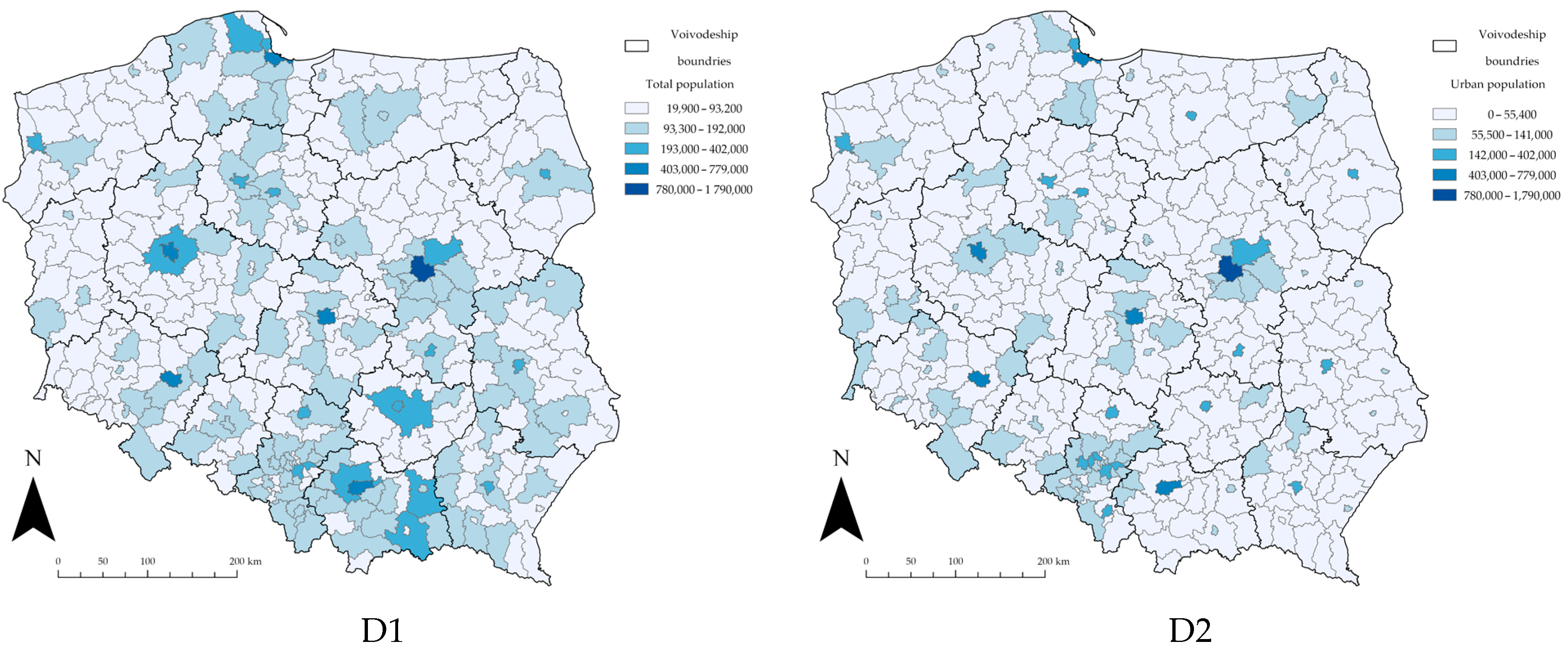
| Demographic | Total population | D1 |
| Urban population | D2 | |
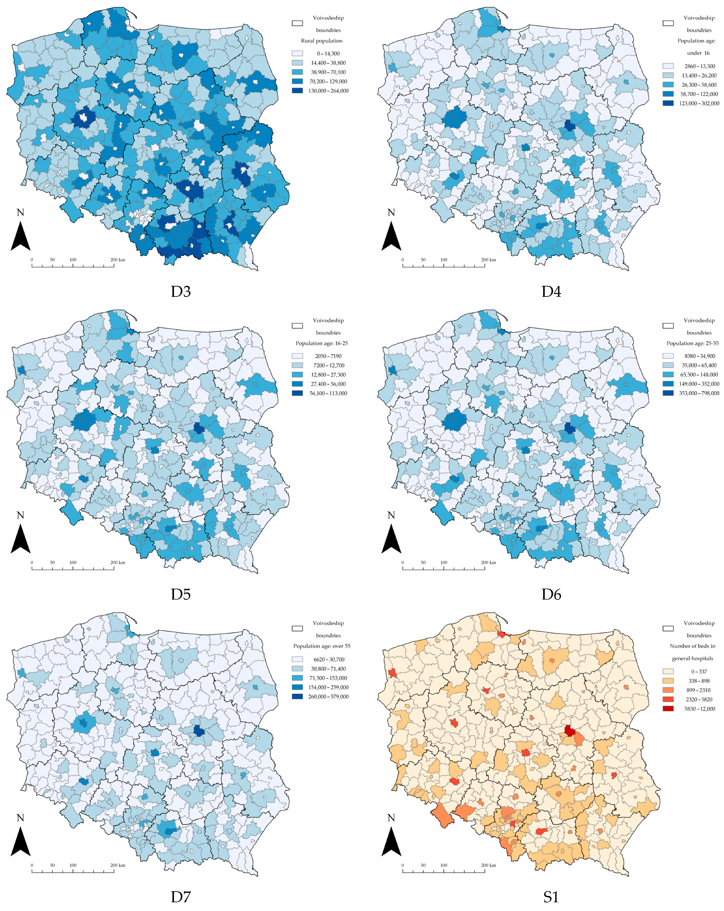
| Rural population | D3 | |
| Population age: under 16 | D4 | |
| Population age: 16–25 | D5 | |
| Population age: 25–55 | D6 | |
| Population age: over 55 | D7 | |
| Social | Number of beds in general hospitals | S1 |
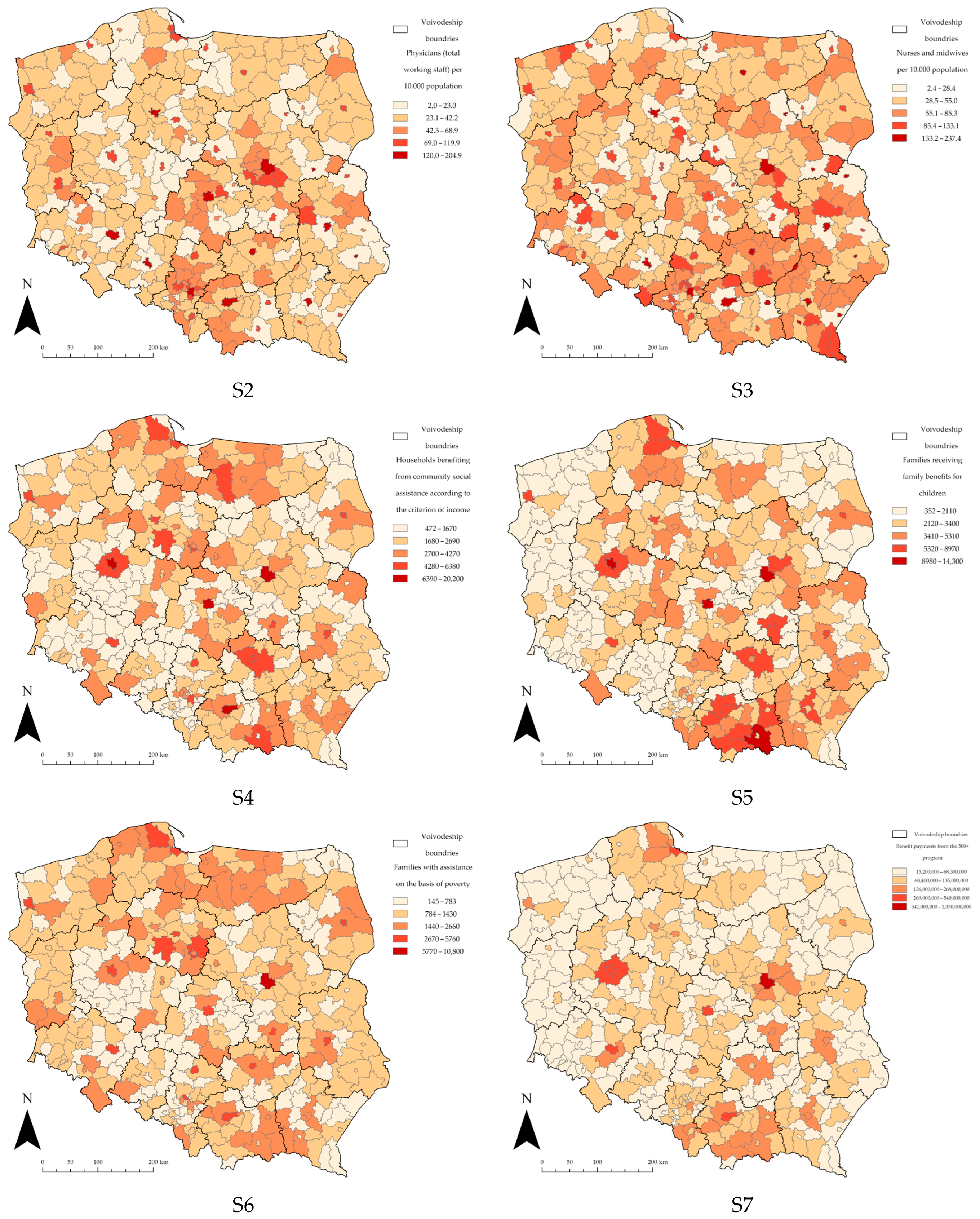
| Physicians (total working staff) per 10,000 population | S2 | |
| Nurses and midwives per 10,000 population | S3 | |
| Households benefiting from community social assistance according to the criterion of income | S4 | |
| Families receiving family benefits for children | S5 | |
| Families with assistance on the basis of poverty | S6 | |
| Benefit payments from the 500+ program | S7 | |
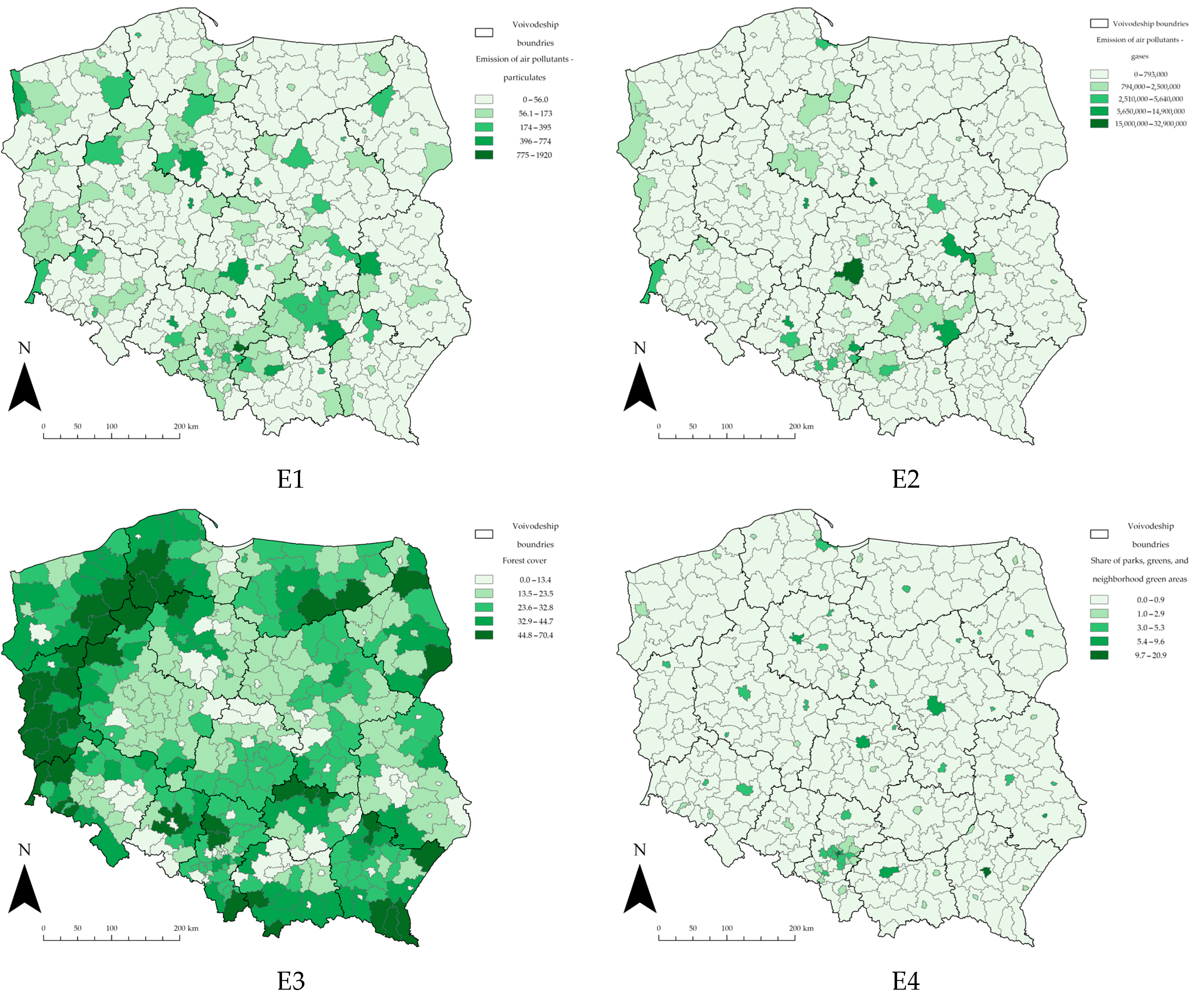
| Environmental | Emission of air pollutants—particulates | E1 |
| Emission of air pollutants—gases | E2 | |
| Forest cover | E3 | |
| Share of parks, greens, and neighborhood green areas | E4 |
| Variable Type | Variable | p-Value | Z-Score | Spatial Pattern | Confidence Level |
|---|---|---|---|---|---|
| Dependent | COVID-19 cases | 0.00 | 5.63 | Clustered | 1% |
| Explanatory | D1—Total population | 0.00 | 4.00 | Clustered | 1% |
| D2—Urban population | 0.01 | 2.62 | Clustered | 1% | |
| D3—Rural population | 0.00 | −3.94 | Dispersed | 1% | |
| D4—Population age: under 16 | 0.00 | 5.53 | Clustered | 1% | |
| D5—Population age: 16–25 | 0.00 | 4.86 | Clustered | 1% | |
| D6—Population age: 25–55 | 0.00 | 4.19 | Clustered | 1% | |
| D7—Population age: over 55 | 0.01 | 2.79 | Clustered | 1% | |
| S1—Number of beds in general hospitals | 0.00 | 3.46 | Clustered | 1% | |
| S2—Physicians (total working staff) per 10,000 population | 0.00 | −3.04 | Dispersed | 1% | |
| S3—Nurses and midwives per 10,000 population | 0.00 | −4.67 | Dispersed | 1% | |
| S4—Households benefiting from community social assistance according to the criterion of income | 0.00 | 2.95 | Clustered | 1% | |
| S5—Families receiving family benefits for children | 0.00 | 6.30 | Clustered | 1% | |
| S6—Families with assistance on the basis of poverty | 0.00 | 3.29 | Clustered | 1% | |
| S7—Benefit payments from the 500+ program | 0.00 | 6.24 | Clustered | 1% | |
| E1—Emission of air pollutants—particulates | 0.02 | 2.41 | Clustered | 5% | |
| E2—Emission of air pollutants—gases | 0.03 | 2.24 | Clustered | 5% | |
| E3—Forest cover | 0.00 | 10.41 | Clustered | 1% | |
| E4—Share of parks, greens, and neighborhood green areas | 0.00 | 3.96 | Clustered | 1% |
| Variable | R2 | Mean | Min | Max | STD |
|---|---|---|---|---|---|
| D1—Total population | 0.99 ** | 101,006.8 | 19,914.0 | 1,790,658.0 | 119,730.5 |
| D2—Urban population | 0.95 ** | 60,613.3 | 0.0 | 1,790,658.0 | 122,692.5 |
| D3—Rural population | 0.37 ** | 40,393.4 | 0.0 | 264,014.0 | 35,060.6 |
| D4—Population age: under 16 | 0.98 ** | 16,433.6 | 2855.0 | 301,697.0 | 19,744.3 |
| D5—Population age: 16–25 | 0.97 ** | 9143.9 | 2054.0 | 112,725.0 | 8220.1 |
| D6—Population age: 25–55 | 0.99 ** | 43,570.8 | 8382.0 | 797,514.0 | 53,035.6 |
| D7—Population age: over 55 | 0.98 ** | 31,858.4 | 6623.0 | 578,722.0 | 39,298.0 |
| S1—Number of beds in general hospitals | 0.91 ** | 439.0 | 0.0 | 11,970.0 | 907.7 |
| S2—Physicians (total working staff) per 10,000 population | 0.73 ** | 41.1 | 2.0 | 204.9 | 30.4 |
| S3—Nurses and midwives per 10,000 population | 0.66 ** | 60.6 | 2.4 | 237.4 | 37.5 |
| S4—Households benefiting from community social assistance according to the criterion of income | 0.94 ** | 2171.1 | 472.0 | 20,186.0 | 1698.4 |
| S5—Families receiving family benefits for children | 0.86 ** | 2653.0 | 352.0 | 14,260.0 | 1739.9 |
| S6—Families with assistance on the basis of poverty | 0.91 ** | 1139.2 | 145.0 | 10,765.0 | 885.6 |
| S7—Benefit payments from the 500+ program | 0.97 ** | 80,276,961.1 | 15,183,262.0 | 1,366,004,134.0 | 90,144,295.6 |
| E1—Emission of air pollutants—particulates | 0.72 * | 71.3 | 0.0 | 1924.0 | 143.3 |
| E2—Emission of air pollutants—gases | 0.70 * | 522,212.5 | 0.0 | 32,882,772.0 | 2,138,844.5 |
| E3—Forest cover | 0.02 ** | 26.0 | 0.0 | 70.4 | 13.4 |
| E4—Share of parks, greens, and neighborhood green areas | 0.83 ** | 0.8 | 0.0 | 20.9 | 1.9 |
| Variable | D1 | D2 | D3 | D4 | D5 | D6 | D7 | S1 | S2 | S3 | S4 | S5 | S6 | S7 | E1 | E2 | E3 | E4 |
|---|---|---|---|---|---|---|---|---|---|---|---|---|---|---|---|---|---|---|
| Residual z-score | −1.26 | −1.28 | 0.66 | −1.95 | −1.44 | −1.82 | −1.93 | −1.46 | 1.35 | −0.81 | −0.34 | 0.73 | 1.33 | −1.7 | 0.75 | 0.33 | 0.38 | 0.01 |
| Spatial pattern | R | R | R | wD | R | wD | wD | R | R | R | R | R | R | wD | R | R | R | R |
Publisher’s Note: MDPI stays neutral with regard to jurisdictional claims in published maps and institutional affiliations. |
© 2022 by the authors. Licensee MDPI, Basel, Switzerland. This article is an open access article distributed under the terms and conditions of the Creative Commons Attribution (CC BY) license (https://creativecommons.org/licenses/by/4.0/).
Share and Cite
Rząsa, K.; Ciski, M. Influence of the Demographic, Social, and Environmental Factors on the COVID-19 Pandemic—Analysis of the Local Variations Using Geographically Weighted Regression. Int. J. Environ. Res. Public Health 2022, 19, 11881. https://doi.org/10.3390/ijerph191911881
Rząsa K, Ciski M. Influence of the Demographic, Social, and Environmental Factors on the COVID-19 Pandemic—Analysis of the Local Variations Using Geographically Weighted Regression. International Journal of Environmental Research and Public Health. 2022; 19(19):11881. https://doi.org/10.3390/ijerph191911881
Chicago/Turabian StyleRząsa, Krzysztof, and Mateusz Ciski. 2022. "Influence of the Demographic, Social, and Environmental Factors on the COVID-19 Pandemic—Analysis of the Local Variations Using Geographically Weighted Regression" International Journal of Environmental Research and Public Health 19, no. 19: 11881. https://doi.org/10.3390/ijerph191911881