
The Volatility of the “Green” Option-Adjusted Spread: Evidence before and during the Pandemic Period


Department of Economic Studies, “G. d’Annunzio” Chieti-Pescara (Italy), 65127 Pescara, Italy
*
Author to whom correspondence should be addressed.
Risks 2022, 10(3), 45; https://doi.org/10.3390/risks10030045
Submission received: 31 December 2021
/
Revised: 15 February 2022
/
Accepted: 16 February 2022
/
Published: 22 February 2022
(This article belongs to the Special Issue Credit Risk Management)
Abstract
:The paper is an investigation on the impact of financial markets on the volatility of the green bonds credit risk component, measured by the option-adjusted spread/swap curve (OAS) before and during the pandemic period. To this purpose, after observing the dynamic joint correlations between all the variables, we adopt Exponential and Generalized AutoRegressive Conditional Heteroskedasticity models, putting the OAS as dependent variable. Our main results show that the conditional variance parameters are significant and persistent in both times, testifying the overall impact of the other markets on the OAS. In more detail, we highlight that the gamma in the two Exponential models is positive: so, the “green” credit risk volatility is more sensitive to positive shocks than to negative ones. With reference to the conditional mean, we note that if during the non-pandemic period only the stock market is significant, during the pandemic also conventional bonds and gold are impacting. To the best of our knowledge this is the first study that analyzes the specific credit risk component of the green bond yields: we deem our findings useful to observe the change of green bonds creditworthiness in a complex market context and interesting in terms of policy implications.
1. Introduction
Motivation Green bonds are deemed useful tools to implement the intertemporal burden sharing of climate mitigation across generations (Flaherty et al. 2017; Orlov et al. 2017; Andersen et al. 2016; Sachs 2014) and to finance the development of the low-carbon transition (Monasterolo and Raberto 2018). Empirically, the emergence and diffusion of the market is justified by three main factors (Monk and Perkins 2020):
- –
- the strategic involvement of intermediaries and entrepreneurs
- –
- some self-reinforcing processes, such as learning, positive externalities and legitimation
- –
- the creation of a more favorable selection environment for sustainable fixed-income products.
Consistently, the attractiveness of these bonds is testified by the exponential growth that the market has recorded, even during the pandemic period. More specifically, even though the sustainable bond market has been characterized by a further split in its themes, on behalf to social, sustainable and pandemic bonds, the green segment has shown an increasing demand and better performances compared to plain vanilla debt instruments. In particular, over the 2020 the market has had a discontinuous trend: if in the first quarter its volume has dropped lower than a half of 2019 (Climate Bonds Initiative 2020a), in the third quarter of 2020 green bonds have reached the highest volume of issuance for a third quarter, i.e., 69.4 bn USD (Climate Bonds Initiative 2020b). Looking to 2021, at the end of the third quarter, the total issuance has reached USD 354.2 bn and it has shown a growth of 15.8% compared with Q3 2020 (Climate Bonds Initiative 2021a).
In general, the attention of investors for sustainability is reflected by the impact on risk premia and their linkage with the creditworthiness of issuers (Höck et al. 2020). In this context, firms with lower carbon emissions seem to limit their default risk (Kabir et al. 2021).
In more detail, over the post-covid inflationary environment, investors have put caution on the possibility that their returns could be eroded; notwithstanding, in the first semester of 2021 rates have remained low, thanks to the ongoing support of central banks and of other pandemic measures, contributing to bond price rising. Specifically, analyzing green bonds yields, researchers have observed a premium, called the “greenium”, that investors are willing to pay in order to make a sustainable investment (e.g., Hyun et al. 2020; Zerbib 2019): in this sense the cost of debt should be lower than the conventional one. In particular, this phenomenon is typical of the primary market: the price of new issuance is higher than the outstanding debt. However, the market has shown larger spread compression than the plain vanilla’s one: in the first half of 2021 it has tightened 24.4 bps (29.9 bps) for the EUR (USD) segment, compared to the 19.6 (24.8) bps of the plain vanilla bonds (Climate Bonds Initiative 2021b). This issue is explainable by the oversubscriptions of green bonds compared with the ongoing lack of supply.
With reference to the overall fixed income market, credit risk has raised up during the pandemic period and has shown up and down correlations with the epidemic trend; however, the levels reached are definitely lower than those recorded during the Financial Crisis (Byström 2021).
Rationale of the study Our focus is on the credit risk component of green bonds’ yield-to-maturity, namely the spread designed to compensate investors for expected loss from a default: to this purpose, we observe the option-adjusted spread/swap curve of the Global Bloomberg Barclays MSCI Green Bond Index. Generally speaking, a yield spread for a bond is calculated by subtracting the yield of a “risk-free” bond. This difference is partly due to the credit risk of corporate bonds, that is why it is frequently referred to as a “credit spread”. The option-adjusted spread (hereinafter OAS) is an improvement on the standard calculation of a yield spread, since it accounts for the possibility that the embedded option in a bond can influence the future cash flows and the overall value of the bond, because of the changes in interest rates. In particular, enclosed options can let the issuer to call back the debt early or the investor to convert the bond into underlying company shares or demand early redemption. The OAS value is commonly expressed as a spread over the Treasury curve and possesses the benefit of allowing for the comparability between bonds with different redemption structures (Boliari and Topyan 2022; CDIAC 2020). It is the spread that must be added to obtain the theoretical price of a corporate bond, as calculated by the pricing model, identical to the observed market price (Choudhry 2004). All in all, as stated by Cavallo and Valenzuela (2007) the option-adjusted spread “simultaneously considers credit risk and cash flow risk, and it is a useful tool for determining an investor’s compensation conditional on the structure of the bond”.
The analysis of the credit risk component of green bonds, cannot disregard the co-movement of the latter and other financial markets (Reboredo 2018) and how it changes over time (Arif et al. 2021). Starting from the interconnections between green and conventional bonds, Broadstock and Cheng (2019), observing the period 28 November 2008–31 July 2018, find three phases in the connection between the two markets: the first shows a shift from negative to positive correlation in mid-2013; across phases one and two there is no strong adjustment in the significance of the determinants; finally the third, that starts in the mid-2016, evidences that macroeconomic conditions increase their role in the connection between green and conventional bond price benchmarks. Zerbib (2019) finds that the non-pecuniary motivates (especially pro-environmental preferences) grant a significant, but low, premium that highlights the opportunity for issuers to expand their bondholders. Nanayakkara and Colombage (2019), analyzing the option-adjusted spread of both kinds of bonds, show that the green ones are traded at a premium of at least 63 bps, stating the investors’ interest for these instruments as a source of portfolio diversification; similarly, Hachenberg and Schiereck (2018) find that rating classes AA–BBB of green bonds, trade marginally tighter for the respective period compared to non-green ones of the same issuers. With reference to the spillovers with the stock and commodity markets, Dutta et al. (2021) analyze the time-varying correlations between climate bonds and US equities, crude oil and gold: they find bidirectional volatility linkage between the first and the latter variables and they state that the hedging portfolio role of climate bonds decreases during the pandemic period. Naeem et al. (2021) document the asymmetric relationship between green bonds and commodities and confirm the diversification benefit of including the first to a commodity portfolio. Reboredo and Ugolini (2020) observe that green bonds are closely linked to the fixed-income and currency markets, receiving sizeable price spillovers from them; on the other side, they find weak connection to stock, energy and high-yield corporate bond markets. Finally, literature has proved the interrelations of green bonds with cryptocurrencies. In this field, Naeem and Karim (2021) find extreme dependence between the two markets, characterized by multiple tail-dependence regimes; they also affirm the hedging effectiveness of green financial assets for bitcoin. Huynh et al. (2020) investigate the role of Artificial Intelligence, robotics stocks and green bonds in portfolio diversification and observe that these assets exhibit heavy-tail dependence and higher volatility transmission in the short-term.
In our study, however, the focus on the OAS aims to find peculiarities for the credit risk of these instruments rather than on their overall performance.
The paper is an investigation on the volatility of the green bonds credit risk component, measured by the option-adjusted spread. In particular, according to the spillovers between these instruments and financial markets, we study the impact of conventional bonds, stocks, oil, gold and cryptocurrencies on the “green” credit risk volatility; the analysis is conducted before and during the pandemic period. To this purpose, after observing the joint dynamic conditional correlations between all the variables through the Dynamic Conditional Correlation Generalized AutoRegressive Conditional Heteroskedasticity (hereinafter DCC-GARCH) model, we adopt Generalized AutoRegressive Conditional Heteroskedasticity (hereinafter GARCH) and Exponential Generalized AutoRegressive Conditional Heteroskedasticity (hereinafter EGARCH) models, putting the OAS as dependent variable.
Contribution Our main results show a joint DCC between variables both in the short and in the long time. In more detail, during the non-pandemic period, only the stock market affects the conditional mean of the “green” adjusted spread; on the other hand, the significance of the conditional volatility parameters, testifies a persistent impact of the one-day lagged performance of the other financial markets, on the current variance of the credit risk component of green bonds. Analogous findings concern the significance of these parameters during the pandemic. In particular we highlight that, in both cases, the gamma of the EGARCH is positive: so, the “green” credit risk volatility is more sensitive to positive shocks than to negative ones. On the contrary, during the pandemic period, we note that the conditional mean estimation is affected by the significant impact of the conventional bonds and gold, added to the role of stocks.
To the best of our knowledge this is the first study that specifically analyzes the credit risk component of green bond yields.
Study’s implications Our findings could be useful to observe the change of green bonds creditworthiness in a complex market context. Moreover, the resilience that green bonds show to negative shocks should enhance the development of the market, to finance private and public investment for the low carbon transition and broader environmental action in the context of the post-pandemic recovery (European Commission 2020). Consistently, policy makers should improve the process of certification and taxonomy of the green products, in order to guarantee the post-issuance transparency.
Finally, the analysis could be proceeded studying bi-directional spillovers of volatility between each market and the “green” credit risk component. Moreover, starting from our global observations, the study could be applied specifically to the European, American and Asian markets.
2. Materials and Methods
The analysis consists in the study of the conditional volatility of the credit risk component of green bonds. Specifically, the variable is analyzed conditioned on the performance of the principal markets connected to the green bond’s one, namely: brown bonds, stocks, gold, oil and cryptocurrencies. The study has been split into two periods:
- pre-pandemic (21 October 2016–7 February 2020)
- pandemic (10 February 2020–29 October 2021).
The dependent variable is represented by the option-adjusted spread/swap curve (OAS) of the Global Bloomberg Barclays MSCI Green Bond Index.
The independent variables are listed below:
- BROWN: quotation of the S&P 500 Bond Index
- FTSE: quotation of the FTSE All-World Index
- GOLD: quotation of the Gold futures
- WTI: quotation of the Crude Oil WTI Futures
- CRYPTO: quotation of the S&P Cryptocurrency MegaCap Index (USD)
Data are daily and their sources are Bloomberg, Datastream and S&P.
The methodology adopted is the univariate conditioned GARCH. More specifically, we implement for each period a GARCH (1,1) and a EGARCH (1,1) model.1
- Conditional GARCH (1,1)
Starting from the Conditional GARCH model, Generalized Autoregressive Conditional Heteroskedasticity (Bollerslev 1986), we calculate the conditional mean and the conditional variance equations, conditioned on the matrix of the independent variables, i.e., MARKETS:
E(OASt/MARKETSt−1) = a + bMARKETSt−1 + εt
E(σ2t/MARKETSt−1) = ω + α E(ε2t−1/MARKETSt−1) + βE
(σ2t−1/MARKETSt−1)
(σ2t−1/MARKETSt−1)
In more detail, in Equation (1), the OAS is expressed as a function of a constant term, “a”, and the one-day lagged value of the matrix MARKETS. Equation (2), instead, expresses the conditional variance dependent on MARKETSt−1, and it denotes the conditioned one-day ahead forecast variance that relies on past information. It is calculated through three terms, namely, a constant one, ω, an ARCH term (ε2t−1/MARKETSt−1) which captures the news about the past period’s volatility conditioned on the independent variables, and the GARCH term (σ2t−1/MARKETSt−1) which denotes the conditioned forecast variance of the last period. The coefficients of the ARCH and GARCH terms (i.e., α and β) are usually summed up to determine the persistence degree of volatility shocks. If the sum is close to one, there is persistence, implying the permanent effect of volatility shocks. If, on the other hand, the sum is significantly less than unity, there is an evidence of a mean-reverting variance process, with shock impacts being just temporary.
- Conditional EGARCH (1,1)
The conditional EGARCH model, is calculated through the Exponential Generalized Autoregressive Conditional Heteroskedasticity (Nelson 1991), conditioned on the MARKETS matrix:
E(ln(σ2t/MARKETSt−1)) = ω + α[E(ε2t−1/σ2t−1)/MARKETSt−1]1/2 + γ[E(ε2t−1/ σ2t−1)/MARKETSt−1]1/2 + β E(ln(σ2t−1/MARKETSt−1))
In particular, γ measures the asymmetric effect. The latter happens if γ is significantly different from zero, with γ < 0 (γ > 0) implying that negative (positive) shocks increase (decrease) volatility greater than positive (negative) shocks of equal magnitude.
In accordance with the non-significance of the Augmented Dickey-Fuller tests for the most of the series, we have calculated their first differences before implementing the models.
Furthermore, we adopt a preliminary analysis of the joint dynamic conditional correlations in the short and long run2 among all variables, through the DCC GARCH (Engle 2002). The details of the model are reported in Appendix A.
3. Results
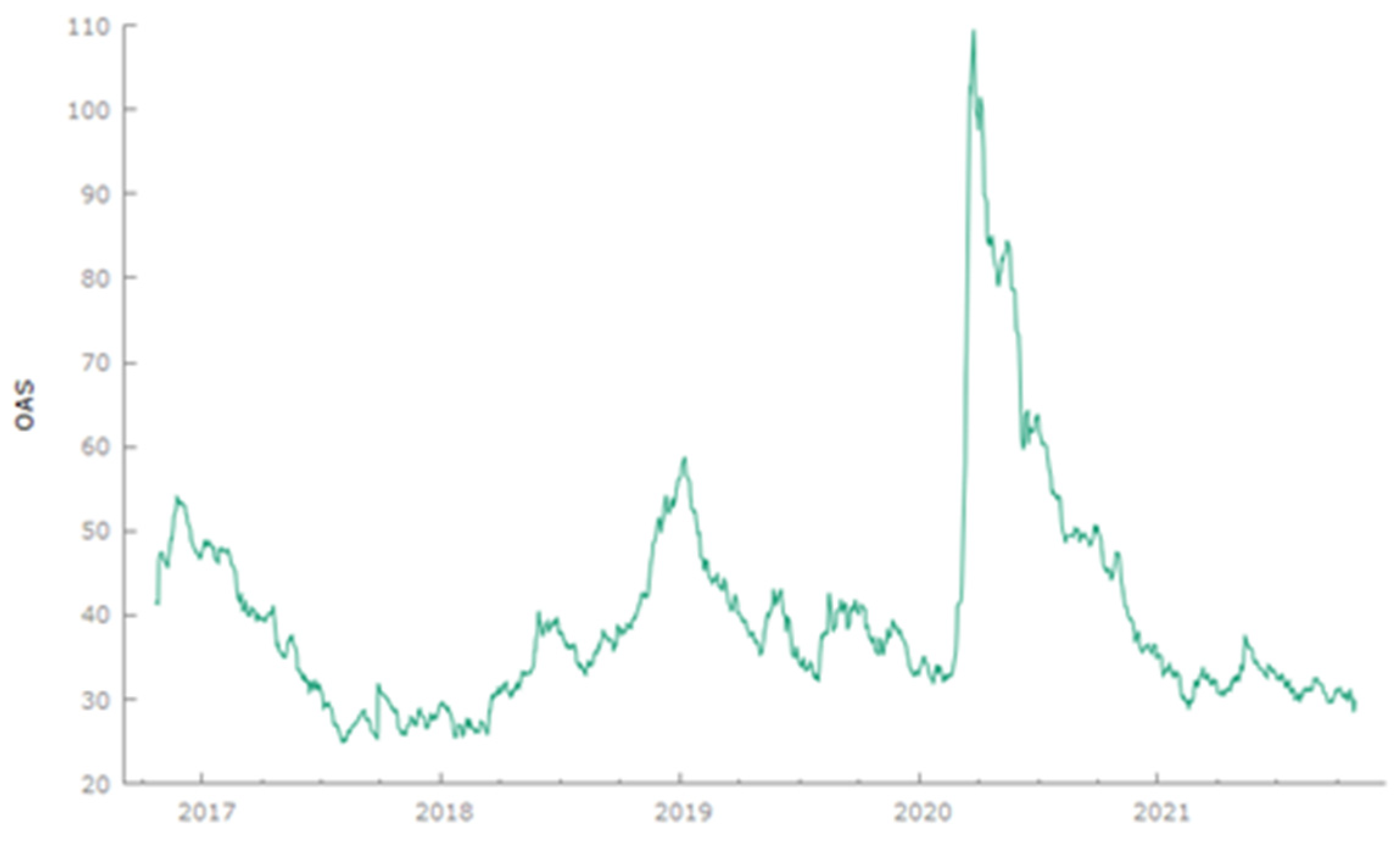
Figure 1 shows graphically the OAS time series over all the period of analysis (10 October 2016–29 October 2021). We note a peak at the beginning of the pandemic, but there is a steep decline in the following months, almost reaching the lowest level shown between 2017 and 2018.
Table 1 and Table 2 illustrate the descriptive statistics, the normality and the unit-root test of the variables, respectively for the non and the pandemic period. We observe that for both times GOLD and CRYPTO have the highest values of standard deviation. As concerns OAS, we note that the standard deviation is quite low, however the value is more than doubled during the pandemic. We also see that the mean of the green bonds’ credit risk component doesn’t change too much between the two times (respectively 37.285 and 45.183), while the maximum value is almost doubled with reference to the pandemic period.
We also highlight that all the variables show a non-normal distribution, as the Jarque-Bera test is significant for both times. Looking to the ADF test, we note that over the non-pandemic period the test is not significant: so all the variables are not stationary; during the pandemic, instead, the test is significant for FTSE and WTI variables.
Table 3 and Table 4 display the correlation matrices for both periods: during the non-pandemic one, OAS shows the highest correlations with the stock market and the crypto index; over the pandemic the correlation grows, and is high also with reference to the bond and oil markets. The OAS presents negative correlations to all the independent variables. Overall, the latter are highly correlated, with a growth during the pandemic. The only exceptions are given by the correlations between GOLD and the OAS and FTSE variables, that decrease (especially in the last case).
Table 5 reports the dynamic parameters of the DCC-GARCH (the details of the model and of the results are illustrated in Appendix A). Specifically, the λ1 and the λ2 express respectively, the short and long run joint dynamic conditional correlation of all the variables. As shown by the table, the results are positively significant in any case.
Table 6 and Table 7 exhibit, respectively, the results of the GARCH(1,1) and EGARCH(1,1) for the non-pandemic and the pandemic period. In particular, the first part of the tables shows the impact of different markets on the conditional mean of the option adjusted spread of green bonds. The second part display the parameters of the conditional variance equation: in particular α and β express, respectively, the ARCH and GARCH coefficients. With reference to the EGARCH, the γ parameter measures the asymmetric reaction of OAS volatility to the independent variables.
Specifically to the non-pandemic period, looking to the information criteria, the values are lower with reference to the GARCH(1,1) model; however, the adoption of the EGARCH, allows us for having an adding information through the γ parameter.
Both GARCH(1,1) and EGARCH(1,1) results for the conditional mean, are characterized by the 1% significance of the only FTSE variable. As concerns the conditional variance equation, the parameters are all significant, with the exception of the constant ω.
With reference to the pandemic, the information criteria would suggest that the GARCH(1,1) model was a bit more efficient than the EGARCH(1,1); notwithstanding, the values are quite similar, so there’s not a model better than the other one.
Looking to the conditional mean equation, the GARCH(1,1) results are characterized by the negative significance of FTSE and BROWN; the parameters of the conditional variance equation are all significant. The EGARCH (1,1) presents similar findings, except for the positive significance of GOLD. Among the results of the conditional variance equation, we highlight the 10% positive significance of the γ.
4. Discussion
The analysis conducted aims to investigate the volatility of the credit risk component of green bonds (the OAS/swap curve), namely the dispersion from its expected value.
The study has considered the co-movements of green bonds with financial markets (Reboredo 2018).
First of all, a preliminary DCC-GARCH analysis has been conducted to illustrate the overall volatility context where green bonds are inserted. In particular, Table 5 shows, for each period, 1% significant lambda parameters: the results testify the short and long run joint dynamic correlations among the overall variables, similarly to Gao et al. (2021). The strict correlations between financial markets have grown after the 2008 crisis and endure for a long time, even in subsequent periods of lower volatility (Sensoy et al. 2013): this is an important issue in terms of potential criticalities for portfolios diversification.
As concerns the core analysis, our main results (see Table 6 and Table 7) show that, if in the non-pandemic period the conditional mean of the “green” credit risk component is affected only by the stock market, during the pandemic, also conventional bonds and gold are significant. Therefore, the one-day lagged values of these variables, are able to predict the expected value of the “green” option-adjusted spread. The negative sign of the BROWN and FTSE variables is quite intuitive: a context of good bond and stock markets, should have a negative relation with credit risk and vice-versa. In particular, the relationship with the conventional bonds expresses a higher sensitivity of the green ones during the pandemic. The result dealing with the stock market, could also have a subtler interpretation: green bonds may not be affected by the takeover risk that characterizes the relation between conventional bonds and stocks. In fact, bondholders could suffer losses in a takeover, especially if funded with debt, causing a positive relationship between stock returns and bond prices (Bhanot et al. 2010). The positive sign of gold is less immediate. However, in this field, Naeem et al. (2021) find mixed signs in the spillovers between the two markets.
With reference to the non-significant variables, our result dealing with WTI, is quite similar to Dutta et al. (2021), who find that climate bonds record a correlation with crude oil near to zero; on the other side, the non-significance of CRYPTO is in contrast with Naeem and Karim (2021), who testify multiple tail-dependence regimes between bitcoin and green bonds.
Looking to the conditional variance, the GARCH and EGARCH show significant parameters in both periods. In particular, the α expresses the impact of the one-day lagged OAS residuals, conditioned on the one-day lagged independent variables, on the OAS volatility in t; the β measures the influence of the one-day lagged OAS volatility, conditioned on the one-day lagged independent variable, on the OAS volatility in t, itself. In both periods, the sum of these parameters is near or even greater than one (see Table 6 and Table 7): this means that there is a persistence in volatility of the “green” credit risk component, conditioned on the other financial markets. Our findings differ from Ferrer et al. (2021), who show that the connectedness between the green bond market and the other ones, mainly occurs at short time horizons, suggesting that shocks are rapidly transmitted across markets with an effect lasting less than a week.
Another interesting result is the positive significance of the γ parameter in the EGARCH model of each period (see Table 6 and Table 7). This is particularly important, because testifies the asymmetry of the “green” OAS, consistently to Park et al. (2020). Specifically, the positive sign means that the “green” credit risk volatility is more sensitive to positive shocks than to negative ones, like the pandemic.
Finally, we observe that while the impact of the independent variables on the conditional mean changes from the non to the pandemic period, it is the same with reference to the conditional variance.
5. Policy Implications
Among our results, we believe that the positive asymmetry of the γ parameter is the one that mostly establishes some policy implications. In fact, this characteristic expresses the resilience of green bonds to negative shocks. This issue is an incentive for investors to choose a kind of financial product useful to reduce the global coal consumption, raise the share of non-fossil electricity and avoid global CO2 emissions (Glomsrød and Wei 2018) and build a more sustainable economy (Tu et al. 2020a, 2020b; Tolliver et al. 2020a, 2020b). For this reason, policy makers have a fundamental role in order to remove the “greenwashing” criticalities, bridging the gap due to the shortcomings of the post-issuance reporting (Tuhkanen and Vulturius 2020). Specifically, enhancing the external certification and labelling is recommended, in addition to formalizing a more appropriate legal framework specific for this market (Paranque and Revelli 2019).
6. Conclusions
The current paper has analyzed the volatility of the OAS/swap curve of the Global Bloomberg Barclays MSCI Green Bond Index, conditioned on the performance of the other financial markets. The methodology adopted is based on GARCH models. The research has been conducted for both the non and pandemic periods. The study has shown that the conditional mean of the “green” credit component changes its dependence over time. In more detail, after a preliminary implementation of the DCC-GARCH model, we have calculated a GARCH(1,1) and an EGARCH(1,1); we have put the OAS as the dependent variable while the conventional bonds, stocks, gold, oil and cryptocurrencies as independent ones.
Specifically, if in the non-pandemic time only the stock market seems to have a significant influence, during the pandemic one, also conventional bonds and gold are impacting.
With reference to the conditional variance, we note that all parameters are significant for each period, showing the persistent impact of the one-day lagged matrix of the independent variables on the expected variance of OAS. We highlight that the most interesting result is the positive significance of the lambda parameter in the EGARCH(1,1) models, which shows that the volatility of the “green” credit risk component is quite asymmetric and is more sensitive to positive information.
This result could have useful implications for investors, as in bullish contexts green bonds creditworthiness should be particularly robust and inclined to be less volatile; at the same time, even in a bearish market, it should not be very susceptible. For this reason, policy makers should improve the regulation of these instruments in order to enhance the transparency during post-issuance and reduce the “greenwashing” phenomenon.
To the best of our knowledge, this is the first study that focuses the investigation on the credit risk component of green bonds.
The research could be proceeded through a bi-directional analysis between the “green” OAS and each financial market; furthermore, starting from our global results, the study could be applied singularly to the European, American and Asian markets.
Author Contributions
Conceptualization, A.O.; methodology, A.O. and E.N.; software, A.O. and E.N.; validation, A.O. and E.N.; formal analysis, A.O.; investigation, A.O.; resources, A.O.; data curation, A.O.; writing—original draft preparation, A.O.; writing—review and editing, A.O.; supervision, E.N. All authors have read and agreed to the published version of the manuscript.
Funding
This research received no external funding.
Informed Consent Statement
Informed consent was obtained from all subjects involved in the study.
Data Availability Statement
Research data are available from authors upon request.
Acknowledgments
The authors thank the anonymous referees for their helpful suggestions and comments.
Conflicts of Interest
The authors declare no conflict of interest.
Appendix A
We briefly illustrate the Dynamic Conditional Correlation GARCH model (DCC-GARCH), (Engle 2002).
The GARCH-DCC calculation is made by two steps.
The first step deals with the conditional heteroskedasticity. It consists in estimating, for each one of the n series of returns ri,t, its conditional volatility σi,t using a GARCH model. Let Dt be a diagonal matrix with these conditional volatilities, i.e., Dti,i = σi,t and, if i ≠ j, Dti,j = 0. Then the standardized residuals are:
where:
vt ≔ Dt−1(rt − μ)
- rt = n × 1 vector of returns
- μ = n × 1 vector of expected returns
The aforementioned standardized residuals have unit conditional volatility.
Now we define the Constant Conditional Correlation (CCC) (Bollerslev 1990) through the following matrix:
The second step is the Dynamic Conditional Correlation (DCC) itself, i.e., the generalizing CCC model (Bollerslev 1990) that captures the dynamics in the correlation:
Qt = R + λ1 (vt−1v’t−1 − R) + λ2(Qt−1 − R)
So Qti,j is the correlation between ri,t and rj,t
Table A1 and Table A2 show the overall results of the DCC-GARCH for both the non and the pandemic periods.

Table A1.
DCC-GARCH Non-pandemic period.
| Non Pandemic | ||||||
|---|---|---|---|---|---|---|
| OAS | BROWN | FTSE | GOLD | WTI | CRYPTO | |
| Ω | 0.017 *** | 0.005 | 0.199 *** | 0.214 | 0.012 | 10.91 |
| (0.007) | (0.004) | (0.075) | (0.431) | (0.009) | (21.471) | |
| α | 0.000 | 0.025 *** | 0.197 *** | 0.000 | 0.028 *** | 0.120 *** |
| (0.0248) | (0.008) | (0.058) | (0.001) | (0.008) | (0.035) | |
| Β | 0.961 *** | 0.969 *** | 0.762 *** | 0.999 *** | 0.962 *** | 0.879 *** |
| (0.044) | (0.011) | (0.059) | (0.000) | (0.007) | (0.054) | |
| λ1 | 0.001 *** | |||||
| λ2 | 0.986 *** | |||||
| AIC: 0.986 | ||||||
| BIC: 30.270 | ||||||
| SIC: 30.072 | ||||||
| HQC: 30.150 | ||||||
Source: Authors’ calculations. Standard error is indicated in parentheses. *** indicates statistical significance at 1%.
Table A2.
DCC-GARCH Pandemic period.
| Pandemic Period | ||||||
|---|---|---|---|---|---|---|
| OAS | BROWN | FTSE | GOLD | WTI | CRYPTO | |
| ω | 0.033 *** | 0.163 | 1.039 ** | 0.000 | 0.026 | 69.375 |
| (0.014) | (0.100) | (0.370) | (0.001) | (0.075) | (63.440) | |
| α | 0.327 *** | 0.260 *** | 0.186 *** | 0.008 *** | 0.056 *** | 0.092 *** |
| (0.086) | (0.098) | (0.057) | (0.001) | (0.013) | (0.025) | |
| β | 0.672 *** | 0.709 *** | 0.752 *** | 0.990 *** | 0.943 *** | 0.907 *** |
| (0.052) | (0.092) | (0.054) | (0.001) | (0.030) | (0.034) | |
| λ1 | 0.0198 *** | |||||
| λ2 | 0.8816 *** | |||||
| AIC: 37.116 | ||||||
| BIC: 37.441 | ||||||
| SIC: 37.105 | ||||||
| HQC: 37.244 | ||||||
Source: Authors’ calculations. Standard error is indicated in parentheses. *** and ** indicate statistical significance at 1% and 5% level, respectively.
| 1 | We have carried out the Weighted ARCH LM Tests that tesfify the adequacy of the order of the two models. |
| 2 | For example we cite some researches that validate the DCC-application for the long run: Ghosh et al. (2020); Fang et al. (2018); Asgharian et al. (2016); Kebalo (2014). |
References
- Andersen, Torben M., Joydeep Bhattacharya, and Pan Liu. 2016. Resolving Intergenerational Conflict over the Environment under the Pareto Criterion. In CESifo Working Paper Series 6053. Munich: CESifo. [Google Scholar]
- Arif, Muhammad, Hasan Mudassar, Suha M. Alawi, and Naeem Muhammad Abubakr. 2021. COVID-19 and time-frequency connectedness between green and conventional financial markets. Global Finance Journal 49: 100650. [Google Scholar] [CrossRef]
- Asgharian, Hossein, Charlotte Christiansen, and Ai Jun Hou. 2016. Macro-Finance Determinants of the Long-Run Stock–Bond Correlation: The DCC-MIDAS Specification. Journal of Financial Econometrics 14: 617–42. [Google Scholar] [CrossRef]
- Bhanot, Karan, Sattar A. Mansi, and K. Wald John. 2010. Takeover risk and the correlation between stocks and bonds. Journal of Empirical Finance 17: 381–93. [Google Scholar] [CrossRef]
- Boliari, Natalia, and Kudret Topyan. 2022. Credit Risk in G20 Nations: A Comparative Analysis in International Finance Using Option-Adjusted-Spreads. Journal of Risk and Financial Management 15: 25. [Google Scholar] [CrossRef]
- Bollerslev, Tim. 1986. Generalized autoregressive conditional heteroskedasticity. Journal of Econometrics 31: 307–27. [Google Scholar] [CrossRef] [Green Version]
- Bollerslev, Tim. 1990. Modeling The Coherence in Short-Run Nominal Exchange Rates: A Multivariate Generalized ARCH Model. Review of Economics and Statistics 72: 498–505. [Google Scholar] [CrossRef]
- Broadstock, David C., and Louis T. W. Cheng. 2019. Time-varying relation between black and green bond price benchmarks: Macroeconomic determinants for the first decade. Finance Research Letters 29: 17–22. [Google Scholar]
- Byström, Hans. 2021. Credit Risk in a Pandemic. The Journal of Fixed Income Fall 31: 48–67. [Google Scholar] [CrossRef]
- Cavallo, Eduardo, and Patricio Valenzuela. 2007. The Determinants of Corporate Risk in Emerging Markets: An Option-Adjusted Spread Analysis. IMF Working Paper 07/228. Available online: https://ssrn.com/abstract=1033210 (accessed on 21 January 2022).
- CDIAC. 2020. Issue Brief: Benefits and Limitations of Option-Adjusted Spread Analysis 20-10. Available online: https://www.treasurer.ca.gov/cdiac/publications/issue-brief/2020/20-10.pdf (accessed on 21 January 2022).
- Choudhry, Moorad. 2004. Advanced Fixed Income Analysis. Amsterdam: Elsevier Butterworth-Heinemann. [Google Scholar]
- Climate Bond Initiative. 2021a. Sustainable Debt Market. Summary Q3 2021. Available online: https://www.climatebonds.net/resources/reports/sustainable-debt-summary-q3-2021 (accessed on 12 August 2021).
- Climate Bond Initiative. 2021b. Green Bond Pricing in the Primary Market: January–June 2021. Available online: https://www.climatebonds.net/resources/reports/green-bond-pricing-primary-market-h1-2021 (accessed on 20 December 2021).
- Climate Bonds Initiative. 2020a. Green Bond Market Summary Q3 2020. Available online: https://www.climatebonds.net/resources/reports/green-bonds-market-summary-q3-2020 (accessed on 10 February 2021).
- Climate Bonds Initiative. 2020b. Sustainable Debt. Global State of the Market H1. Available online: https://www.climatebonds.net/resources/reports/sustainable-debt-global-state-market-2020 (accessed on 10 February 2021).
- Dutta, Aupam, Elie Bouri, and Md Hasib Noor. 2021. Climate bond, stock, gold, and oil markets: Dynamic correlations and hedging analyses during the COVID-19 outbreak. Resources Policy 74: 102265. [Google Scholar] [CrossRef] [PubMed]
- Engle, Robert. 2002. Dynamic Conditional Correlation: A Simple Class of Multivariate Generalized Autoregressive Conditional Heteroskedasticity Models. Journal of Business & Economic Statistics 20: 339–50. [Google Scholar]
- European Commission. 2020. Financing a Sustainable Recovery with Green Bonds. Science for Brief Policy. Available online: https://ec.europa.eu/jrc/sites/default/files/jrc122441_gb_scienceforpolicybrief_revised1.pdf (accessed on 2 February 2022).
- Fang, Libing, Baizhu Chen, Honghai Yu, and Cheng Xiong. 2018. The effect of economic policy uncertainty on the long-run correlation between crude oil and the U.S. stock markets. Finance Research Letters 24: 56–63. [Google Scholar] [CrossRef]
- Ferrer, Romàn, Syed Jawad Hussain Shahzad, and Pillar Soriano. 2021. Are green bonds a different asset class? Evidence from time-frequency. Journal of Cleaner Production 292: 125988. [Google Scholar] [CrossRef]
- Flaherty, Michael, Arkady Gevorkyan, Siavash Radpour, and Willi Semmler. 2017. Financing climate policies through climate bonds—A three stage model and empirics. Research in International Business and Finance 42: 468–79. [Google Scholar] [CrossRef]
- Gao, Yang, Yangyang Li, and Yaojun Wang. 2021. Risk spillover and network connectedness analysis of China’s green bond and financial markets: Evidence from financial events of 2015–2020. North American Journal of Economics and Finance 57: 101386. [Google Scholar] [CrossRef]
- Ghosh, Indranil, Manas K. Sanyal, and R. K. Jana. 2020. Co-movement and Dynamic Correlation of Financial and Energy Markets: An Integrated Framework of Nonlinear Dynamics, Wavelet Analysis and DCC-GARCH. Computational Economics 57: 503–27. [Google Scholar] [CrossRef]
- Glomsrød, Solveig, and Taoyuan Wei. 2018. Business as unusual: The implications of fossil divestment and green bonds for financial flows, economic growth and energy market. Energy for Sustainable Development 44: 1–10. [Google Scholar] [CrossRef]
- Hachenberg, Britta, and Dirk Schiereck. 2018. Are green bonds priced differently from conventional bonds? Journal of Asset Management 19: 371–83. [Google Scholar] [CrossRef]
- Höck, André, Christian Klein, Alexander Landau, and Bernhard Zwergel. 2020. The effect of environmental sustainability on credit risk. Journal of Asset Management 21: 85–93. [Google Scholar] [CrossRef]
- Huynh, Toan Luu Duc, Erik Hille, and Muhammad Ali Nasir. 2020. Diversification in the age of the 4th industrial revolution: The role of artificial intelligence, green bonds and cryptocurrencies. Technological Forecasting & Social Change 159: 120188. [Google Scholar]
- Hyun, Suk, Donghyun Park, and Shu Tian. 2020. The price of going green: The role of greenness in green bond markets. Accounting & Finance 60: 73–95. [Google Scholar]
- Kabir, Md Nurul, Rahman Sohanur, Rahman Md Arifur, and Anwar Mumtaheena. 2021. Carbon emissions and default risk: International evidence from firm-level data. Economic Modelling 103: 105617. [Google Scholar] [CrossRef]
- Kebalo, Leleng. 2014. What DCC-GARCH Model Tell Us about the Effect of the Gold Price’s Volatility on South African Exchange Rate? MPRA Paper No. 72584. Available online: https://mpra.ub.uni-muenchen.de/72584/ (accessed on 14 October 2021).
- Monasterolo, Irene, and Marco Raberto. 2018. The EIRIN Flow-of-funds Behavioural Model of Green Fiscal Policies and Green Sovereign Bonds. Ecological Economics 144: 228–43. [Google Scholar] [CrossRef]
- Monk, Alexander, and Richard Perkins. 2020. What explains the emergence and diffusion of green bonds? Energy Policy 145: 111641. [Google Scholar] [CrossRef]
- Naeem, Muhammad Abubakr, and Sitara Karim. 2021. Tail dependence between bitcoin and green financial assets. Economics Letters 208: 110068. [Google Scholar] [CrossRef]
- Naeem, Muhammad Abubakr, Thi Thu Nguyen, Rabindra Nepal, Quang-Thanh Ngo, and Farhad Taghizadeh–Hesary. 2021. Asymmetric relationship between green bonds and commodities: Evidence from extreme quantile approach. Finance Research Letters 43: 101983. [Google Scholar] [CrossRef]
- Nanayakkara, Madurika, and Sisira Colombage. 2019. Do investors in Green Bond market pay a premium? Global evidence. Applied Economics 51: 4425–37. [Google Scholar] [CrossRef]
- Nelson, Daniel B. 1991. Conditional heteroskedasticity in asset returns: A new approach. Econometrica 59: 347–70. [Google Scholar] [CrossRef]
- Orlov, Sergey, Elena Rovenskaya, Julia Puaschunder, and M. Semmler Willi. 2017. Green Bonds, Transition to a Low-Carbon Economy, and Intergenerational Fairness: Evidence from an Extended DICE Model. Available online: https://ssrn.com/abstract=3086483 (accessed on 24 January 2022).
- Paranque, Benanrd, and Christophe Revelli. 2019. Ethico-economic analysis of impact finance: The case of Green Bonds. Research in International Business and Finance 47: 57–66. [Google Scholar] [CrossRef]
- Park, Daehyeon, Jiyeon Park, and Doojin Ryu. 2020. Volatility Spillovers between Equity and Green Bond Markets. Sustainability 12: 3722. [Google Scholar] [CrossRef]
- Reboredo, Juan C. 2018. Green bond and financial markets: Co-movement, diversification and price spillover effects. Energy Economics 74: 38–50. [Google Scholar]
- Reboredo, Juan C., and Andrea Ugolini. 2020. Price connectedness between green bond and financial markets. Economic Modelling 88: 25–38. [Google Scholar] [CrossRef]
- Sachs, Jeffrey D. 2014. Climate change and intergenerational well-being. In The Oxford Handbook of the Macroeconomics of Global Warming. Edited by Lucas Bernard and Willi Semmler. Oxford: Oxford University Press, pp. 248–59. [Google Scholar]
- Sensoy, Ahmet, Serdar Yuksel, and Mutahhar Erturk. 2013. Analysis of cross-correlations between financial markets after the 2008 crisis. Physica A 392: 5027–45. [Google Scholar] [CrossRef]
- Tolliver, Clarence, Alexander Ryota Keeley, and Shunsuke Managi. 2020a. Drivers of green bond market growth: The importance of Nationally Determined Contributions to the Paris Agreement and implications for sustainability. Journal of Cleaner Production 244: 118643. [Google Scholar] [CrossRef]
- Tolliver, Clarence, Alexander Ryota Keeley, and Shunsuke Managi. 2020b. Policy targets behind green bonds for renewable energy: Do climate commitments matter? Technological Forecasting and Social Change 157: 120051. [Google Scholar] [CrossRef]
- Tu, Chuc, Ehsan Rasoulinezhad Anh, and Sarker Tapan. 2020a. Investigating solutions for the development of a green bond market:Evidence from analytic hierarchy process. Finance Research Letters 34: 101457. [Google Scholar] [CrossRef]
- Tu, Chuc, Ehsan Rasoulinezhad Anh, and Sarker Tapan. 2020b. Factors Influencing the Green Bond Market Expansion: Evidence from a Multi-Dimensional Analysis. Journal of Risk and Financial Management 13: 126. [Google Scholar]
- Tuhkanen, Heidi, and Gregor Vulturius. 2020. Are green bonds funding the transition? Investigating the link between companies’ climate targets and green debt financing. Journal of Sustainable Finance & Investment, 1–23. [Google Scholar] [CrossRef]
- Zerbib, Olivier D. 2019. The effect of pro-environmental preferences on bond prices: Evidence from green bonds. Journal of Banking & Finance 98: 39–60. [Google Scholar]
Figure 1.
OAS time series. Source: Authors’ calculations.

Table 1.
Descriptive statistics, Normality and Unit-root test.
| Non-Pandemic Period | ||||||||
|---|---|---|---|---|---|---|---|---|
| Variable | Mean | Min | Max | St. Dev. | Skewness | Kurtosis | JB Test | ADF |
| OAS | 37.285 | 24.811 | 58.677 | 7.579 | 0.475 | −0.333 | 36.189 *** | −1.618 |
| BROWN | 441.564 | 410.08 | 502.06 | 23.465 | 1.088 | −0.072 | 169.305 *** | −0.563 |
| FTSE | 327.246 | 266.43 | 382.32 | 24.521 | −0.428 | −0.176 | 27.317 *** | −2.348 |
| GOLD | 1378.505 | 1134.55 | 1627.3 | 92.186 | 0.785 | −0.010 | 87.942 *** | −1.676 |
| WTI | 57.071 | 42.53 | 76.41 | 7.573 | 0.371 | −0.700 | 37.143 *** | −1.911 |
| CRYPTO | 801.307 | 83.71 | 76.41 | 477.788 | 0.392 | −0.089 | 22.193 *** | −2.326 |
| Obs. 857 | ||||||||
Source: Authors’ calculations. *** indicates statistical significance at 1% level, respectively.
Table 2.
Descriptive statistics, Normality and Unit-root test.
| Pandemic Period | ||||||||
|---|---|---|---|---|---|---|---|---|
| Variable | Mean | Min | Max | St. Dev. | Skewness | Kurtosis | JB Test | ADF |
| OAS | 45.183 | 28.614 | 109.488 | 18.929 | 11.150 | 178.52 | 210.119 *** | −2.143 |
| BROWN | 523.291 | 445.3 | 543.53 | 16.835 | −1.8161 | 4.1938 | 566.8 8 *** | −2.573 |
| FTSE | 409.772 | 253.51 | 491.71 | 59.782 | −0.408 | −0.949 | 28.880 *** | −5.307 *** |
| GOLD | 1812.119 | 1491 | 491.71 | 96.808 | −0.103 | 0.390 | 3.573 *** | −2.173 |
| WTI | 51.4041 | −37.63 | 84.65 | 17.168 | −0.385 | 0.571 | 16.914 *** | −4.003 *** |
| CRYPTO | 3736.643 | 712.43 | 8855.37 | 2496.129 | 0.364 | −1.398 | 45.752 *** | −1.986 |
| Obs. 442 | ||||||||
Source: Authors’ calculations. *** indicates statistical significance at 1% level, respectively.
Table 3.
Correlation matrix for the non-pandemic period.
| OAS | BROWN | FTSE | GOLD | WTI | CRYPTO | |
|---|---|---|---|---|---|---|
| OAS | 1 | |||||
| BROWN | −0.150 | 1 | ||||
| FTSE | −0.481 | 0.706 | 1 | |||
| GOLD | −0.284 | 0.850 | 0.667 | 1 | ||
| WTI | −0.209 | 0.049 | 0.587 | 0.062 | 1 | |
| CRYPTO | −0.484 | 0.539 | 0.767 | 0.569 | 0.507 | 1 |
Source: Authors’ calculations.
Table 4.
Correlation matrix for the pandemic period.
| OAS | BROWN | FTSE | GOLD | WTI | CRYPTO | |
|---|---|---|---|---|---|---|
| OAS | 1 | |||||
| BROWN | −0.808 | 1 | ||||
| FTSE | −0.893 | 0.752 | 1 | |||
| GOLD | −0.237 | 0.603 | 0.146 | 1 | ||
| WTI | −0.831 | 0.625 | 0.934 | 0.299 | 1 | |
| CRYPTO | −0.707 | 0.438 | 0.863 | 0.527 | 0.833 | 1 |
Source: Authors’ calculations.
Table 5.
DCC-GARCH parameters for non and pandemic period.
| Non-Pandemic | Pandemic | |
|---|---|---|
| λ1 | 0.003 *** | 0.020 *** |
| λ2 | 0.986 *** | 0.881 *** |
Source: Authors’ calculations. *** indicates statistical significance at 1% level, respectively.
Table 6.
GARCH(1,1) e EGARCH(1,1) Non-pandemic period.
| GARCH (1,1) | EGARCH (1,1) | ||
|---|---|---|---|
| Conditional mean equation | |||
| const. | −0.011 | −0.003 | |
| (0.024) | (0.023) | ||
| BROWN | 0.001 | 0.014 | |
| (0.03) | (0.022) | ||
| FTSE | −0.087 *** | −0.103 *** | |
| (0.017) | (0.010) | ||
| GOLD | −0.001 | −0.001 | |
| (0.001) | (0.001) | ||
| WTI | 0.014 | 0.023 | |
| (0.029) | (0.019) | ||
| CRYPTO | 0.000 | −0.000 | |
| (0.001) | (0.000) | ||
| Conditional variance equation | |||
| ω | 0.003 | ω | −0.025 |
| α | −0.008 *** | α | −0.027 *** |
| β | 1.002 *** | β | 0.953 *** |
| γ | 0.029 ** | ||
| Llik: | −823.416 | Llik: | −840.811 |
| AIC: | 1664.832 | AIC: | 1701.622 |
| BIC: | 1707.603 | BIC: | 1749.145 |
| HQC: | 1681.210 | HQC: | 1719.819 |
Source: Authors’ calculations. Standard error is indicated in parentheses. *** and ** indicate statistical significance at 1% and 5% level, respectively.
Table 7.
GARCH(1,1) e EGARCH(1,1) Pandemic period.
| GARCH (1,1) | EGARCH (1,1) | ||
|---|---|---|---|
| Conditional mean equation | |||
| const. | −0.0788 *** | −0.036 *** | |
| (0.027) | (0.007) | ||
| BROWN | −0.076 *** | −0.070 *** | |
| (0.025) | (0.008) | ||
| FTSE | −0.076 *** | −0.078 *** | |
| (0.012) | (0.015) | ||
| GOLD | 0.003 | 0.002 ** | |
| (0.002) | (0.001) | ||
| WTI | −0.014 | −0.008 | |
| (0.009) | (0.031) | ||
| CRYPTO | 0.000 | 0.000 | |
| (0.000) | (0.000) | ||
| Conditional variance equation | |||
| ω | 0.034 *** | ω | −0.432 *** |
| α | 0.440 *** | α | 0.558 *** |
| β | 0.606 *** | β | 0.959 *** |
| γ | 0.107 * | ||
| Llik: | −450.451 | Llik: | −452.675 |
| AIC: | 918.901 | AIC: | 925.350 |
| BIC: | 955.703 | BIC: | 966.240 |
| HQC: | 933.418 | HQC: | 941.479 |
Source: Authors’ calculations. Standard error is indicated in parentheses. ***, **, and * indicate statistical significance at 1%, 5%, and 10% level, respectively.
Publisher’s Note: MDPI stays neutral with regard to jurisdictional claims in published maps and institutional affiliations. |
© 2022 by the authors. Licensee MDPI, Basel, Switzerland. This article is an open access article distributed under the terms and conditions of the Creative Commons Attribution (CC BY) license (https://creativecommons.org/licenses/by/4.0/).
Share and Cite
MDPI and ACS Style
Ortolano, A.; Nissi, E. The Volatility of the “Green” Option-Adjusted Spread: Evidence before and during the Pandemic Period. Risks 2022, 10, 45. https://doi.org/10.3390/risks10030045
AMA Style
Ortolano A, Nissi E. The Volatility of the “Green” Option-Adjusted Spread: Evidence before and during the Pandemic Period. Risks. 2022; 10(3):45. https://doi.org/10.3390/risks10030045
Chicago/Turabian StyleOrtolano, Alessandra, and Eugenia Nissi. 2022. "The Volatility of the “Green” Option-Adjusted Spread: Evidence before and during the Pandemic Period" Risks 10, no. 3: 45. https://doi.org/10.3390/risks10030045
Note that from the first issue of 2016, this journal uses article numbers instead of page numbers. See further details here.