Air Pollutant Analysis and AQI Prediction Based on GRA and Improved SOA-SVR by Considering COVID-19

Abstract

Since COVID-19 pneumonia broke out, the Chinese government has taken a series of measures to control the spread of the epidemic, which has made the air quality of Taiyuan in February 2020 significantly better than during the same period in previous years. In this paper, the Gray Relational Analysis (GRA) method was first applied to evaluate and analyze the influence of six major pollutants on air quality. Then, the improved seagull optimization algorithm (ISOA) was proposed and combined with Support Vector Regression (SVR) to establish a hybrid predicted model ISOA-SVR. Finally, the proposed ISOA-SVR was utilized to predict air quality index (AQI). The experimental results on two kinds of different data showed that the proposed ISOA-SVR had the better generalization ability and robustness compared with other predicted models. Further, the proposed ISOA-SVR is suitable for the prediction of AQI.

1. Introduction

With the concentration of urban population and industrial growth, environmental pollution problems are arising. Previous research showed that air pollution has a direct impact on human health. It is estimated that 1.22 million people are killed every year by haze in China, accounting for about 15% of annual deaths [1]. According to the data of the World Health Organization in 2018, air pollution causes seven million people to die of cancer, stroke, heart disease and respiratory diseases every year. Air pollution has become the number one killer of human beings. In 2019, the World Health Organization lists air pollution as one of the top ten threats to global health [2].

Air quality prediction is helpful to prevent air pollution from causing damage, and it can guide government departments to take corresponding preventive measures to prevent serious air pollution, such as heavy polluting enterprises stopping production and traffic restriction. At the same time, it can provide travel suggestions for people’s outdoor activities. Therefore, timely and reliable air quality forecasting is very necessary for the prevention and control of air pollution. Air quality index (AQI) is an important index to reflect and evaluate air quality [3]. According to China’s air quality standard, AQI is obtained from the concentrations of six main pollutants including fine particulate matter (PM_2.5), inhalable particles (PM₁₀), sulfur dioxide (SO₂), carbon monoxide (CO), nitrogen dioxide (NO₂) and ozone(O₃) [4]. The value of the AQI index reflects the level of air quality; a low AQI value means that the air quality is good, and it is conducive to travel, whereas a higher AQI value indicates that the air pollution is serious.

In the face of increasingly serious air pollution problems, people have more and more attention on air quality. An autoregressive moving average (ARIMA) model was used to predict the monthly value of air pollution index and the daily value of AQI in [5,6]. However, if the sequence is nonlinear or irregular, ARIMA may not provide reliable prediction results. Compared with the ARIMA model, Support Vector Regression (SVR) [7,8] has been widely used in nonlinear systems with good generalization ability. Chen et al. used SVR and a multivariate analysis model to analyze daily precipitation [9]. Withing the literature [10,11] SVR has been applied to predict short-term electrical load. Mauro Castelli et al. used an SVR model to predict AQI in California [12]. In the literature [13], an SVR model was used to predict the AQI value of Beijing and NOx values in India. A mixed prediction model based on the combination of fractional grey theory and SVM was established by Meng Dun et al. to predict the concentrations of PM₁₀, PM_2.5 and NO₂ in Shijiazhuang and Chongqing [14]. However, the performance of SVR depends on the choice of SVR model parameters. In other words, the selection of parameters has a great influence on the learning and generalization ability of SVR. Therefore, it is very important to select optimal parameters to obtain good SVR performance. In fact, since the SVR model was proposed, many researchers have given attention to the problem of SVR parameter optimization. In [15,16], the parameters of SVR were optimized by a genetic algorithm (GA). Wang and Zhang used a differential evolution algorithm (DE) to find optimal SVR parameters [17,18]. The optimization of SVR parameters by particle swarm optimization (PSO) have been studied in literature [19,20,21]. In recent years, with the development of various new intelligent algorithms, there are more choices for the optimization algorithm of SVR model parameters. Cao optimized SVR parameters with fruit fly optimization (FFO) [22], and optimization of SVR parameters with gray wolf optimization (GWO) appeared in [23].

In this paper, we first evaluate and analyze the air quality of Taiyuan city, which since the outbreak of COVID-19 has been done using the grey relational analysis (GRA) method [24]. Then, three improvements to the seagull optimization algorithm (SOA) [25] are proposed. First, according to the flight characteristics of seagulls, the control parameters that adjust the seagulls to move to the best position direction are changed from a linear change to an exponential change. Second, considering the influence of individual seagulls and groups, an adaptive nonlinear weight is introduced. Third, seagulls with poor fitness are selected for position random selection update to increase the diversity of samples to avoid local minimum errors in the process of optimization. On this basis, we propose an improved seagull optimization algorithm (ISOA) combined with support vector regression (SVR) to establish a hybrid prediction model ISOA-SVR. Finally, the proposed ISOA-SVR method is used to predict air quality index (AQI). In addition, we combine particle swarm optimization (PSO) [26], sine cosine optimization (SCA) [27], whale optimization (WOA) [28] and an SOA algorithm with SVR, respectively, to establish PSO-SVR, SCA-SVR, WOA-SVR and SOA-SVR, and compare them with the experimental results of ISOA-SVR in turn. The experimental results on two different data sets showed that the proposed ISOA-SVR method had the better performance, and the generalization ability and robustness of the model were proved.

The main structure of this paper is as follows. In Section 2, the grey relational analysis method and SVR model are briefly reviewed. The improved SOA algorithm (ISOA) and proposed ISOA-SVR integration model are introduced in Section 3. Section 4 introduces the experimental materials, including data, experimental environment and evaluation index. Section 5.1 includes the evaluation and analysis of the air quality of Taiyuan city before and after the outbreak of COVID-19 by using the grey relational analysis method. The comparative experiments on the prediction of AQI values using SVR prediction models optimized by different optimization algorithms are arranged in Section 5.2. Finally, Section 6 concludes and discusses the paper.

2. Materials and Methods

2.1. Grey Relational Analysis (GRA)

Grey relational analysis (GRA) is a method to measure the degree of relational between factors according to the degree of similarity or difference in the development trend between them [24]. If the change trend of two factors is consistent, that is, the degree of synchronous change is high, this indicates that the relational degree between the two factors is high; otherwise it is low. The specific steps of the grey relational method are as follows:

Step 1: Determine the analysis sequence.

The reference sequence reflecting the characteristics of system behavior and the data sequence of factors influencing system behavior are determined.

Step 2: Dimensionless variables.

Because the data of each factor column in the system may be different due to different dimensions, it is not convenient to compare, or it is difficult to get the correct results when comparing. Therefore, in order to ensure the reliability of the results, dimensionless processing should be carried out first in the grey relational analysis.

Step 3: Calculate the relational coefficient.

The relational coefficient of comparison sequence $x_i(i=1,2,\cdots n)$ to reference sequence $x_0$ at time $t$ is as follows:

$${\xi }_i(t)=\frac{\underset{i}{\min }({\Delta }_i(\min ))+\rho \underset{i}{\max }({\Delta }_i(\max ))}{\left|x_0(t)-x_i(t)\right|+\rho \underset{i}{\max }({\Delta }_i(\max ))},$$

(1)

where $\rho$ is the resolution coefficient, usually the number in (0, 1).

$$\underset{i}{\min }({\Delta }_i(\min ))=\underset{i}{\min }(\underset{t}{\min }\left|x_0(t)-x_i(t)\right|),$$

(2)

$$\underset{i}{\max }({\Delta }_i(\max ))=\underset{i}{\max }(\underset{t}{\max }\left|x_0(t)-x_i(t)\right|),$$

(3)

Step 4: Calculate the relational degree.

Because the relational coefficient is the value of the relational degree between the comparison sequence and the reference sequence at each time (i.e., each point in the curve), there is more than one of them and the information is too scattered to facilitate the overall comparison. Therefore, it is necessary to concentrate the relational coefficient of each time into one value; that is, to calculate the average value as the quantitative expression of the relational degree between the comparison sequence and the reference sequence. The relational degree is calculated as follows:

$$r_i=\frac{1}{N}{\displaystyle \sum _{t=1}^N{\xi }_i(t)}$$

(4)

Step 5: Rank the relational degree. The larger the value, the stronger the relational.

2.2. Support Vector Regression (SVR)

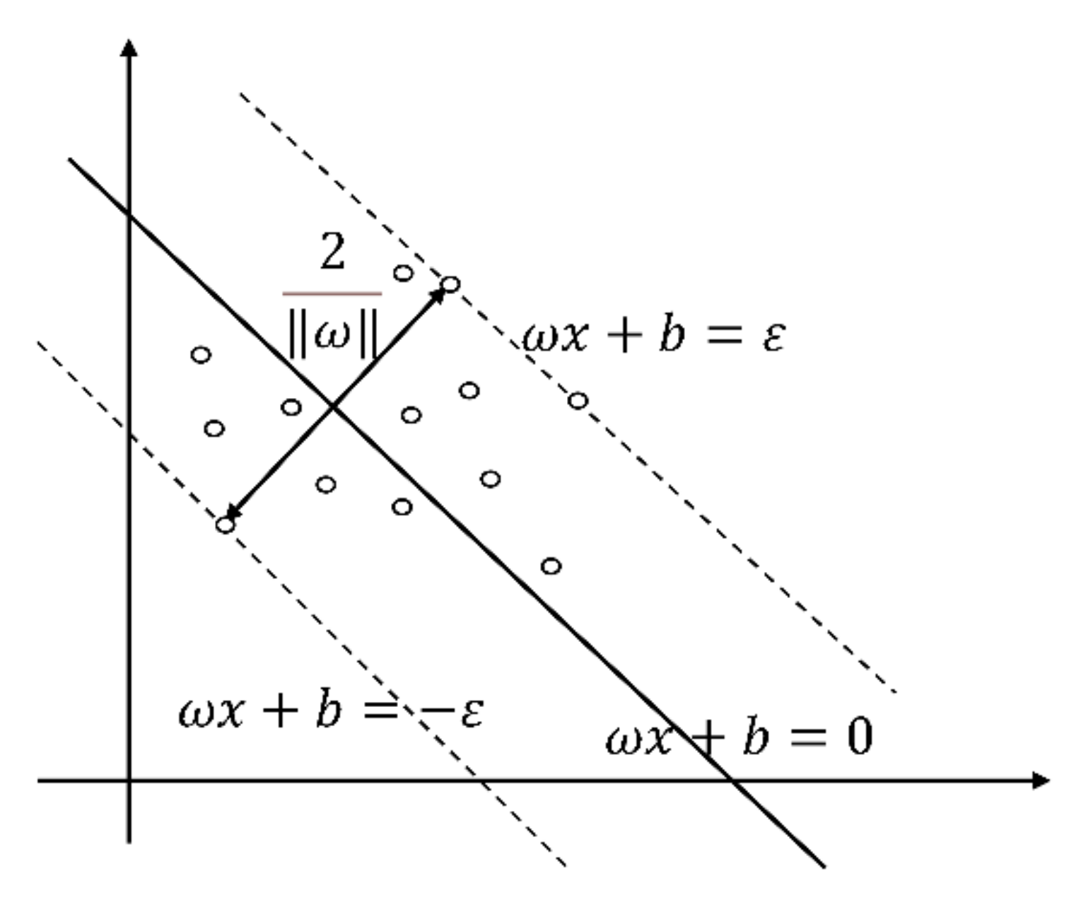
Support Vector Regression (SVR) is a support vector algorithm for regression problems [7]. The goal of SVR is to find an optimal hyperplane, so that the deviations between training data and the hyperplane are not greater than $\epsilon$. In other words, it minimizes the distance between the support vectors on both sides of the hyperplane. A schematic diagram of SVR is shown in Figure 1.

Therefore, a regression function $f(x)$ can be obtained by training SVR so that its deviation from the actual value $y$ is not more than $\epsilon$ for each training vector $x$. The details of the SVR are presented in reference [8]. The regression function $f(x)$ can be obtained as:

$$f(x)={\displaystyle \sum _{i=1}^m(a_i^{\ast }-{\alpha }_i)K(x,x_i})+b$$

(5)

where $x$ is the input feature vector, $b$ is the bias term, ${\alpha }_i^{\ast }$ and ${\alpha }_i$ are Lagrange multipliers and $K(x,x_i)$ is a kernel function with functional forms that can be obtained from the following equations:

$$\begin{array}{l}\mathrm{linear}\mathrm{kernel}\mathrm{function}:K(x,x_i)=x^T{x}_i.\\ \mathrm{polynomial}\mathrm{kernel}\mathrm{function}:K(x,x_i)={(\gamma x^T{x}_i+1)}^d,d\in (1,n),\gamma >0.\\ \mathrm{radial}\mathrm{basis}\mathrm{kernel}\mathrm{function}:K(x,x_i)=\exp (-\gamma {‖x-x_i‖}^2),\gamma >0.\end{array}$$

3. Proposed Method

3.1. Seagull Optimization Algorithm (SOA)

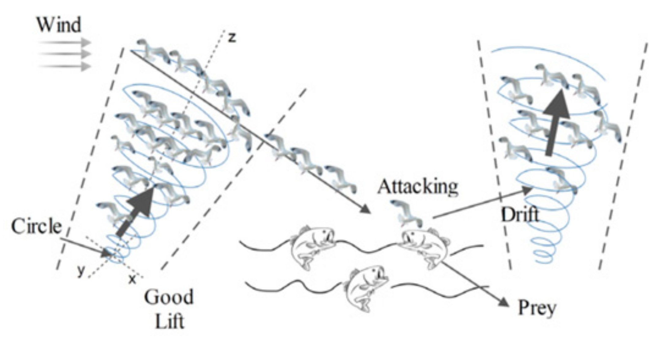
The seagull optimization algorithm (SOA) is a swarm intelligence optimization algorithm proposed by Dhiman and Kumar in 2019 [25]. In this algorithm, the migration of seagulls and the attack behavior in the migration process are regarded as the optimization process of the optimization problem, and the location of seagulls in the algorithm is the potential solution of the optimization problem. The migration and attack patterns of seagulls are shown in Figure 2.

1. Migration behavior of seagulls (global search)

In this part, the algorithm simulates how the group of seagulls move from one position to another. In the process of migration, the movement behavior of seagulls satisfies the following three conditions:

(1).

Collision avoidance. An additional variable A is employed for the calculation of new seagull position to avoid collisions between seagull neighbors.

$$A=a-a(t/T)$$

(6)

$$C=AP$$

(7)

where $C$ is defined as a new position that does not allow collision with other seagulls. The current position of seagulls is represented by $P$. $t$ and $T$ are the current iteration and the maximum number of iterations, respectively.$A$ represents the movement behavior of seagulls in a given search space. The constant $a$ is used to control the range of $A$, when $a=2$. $A$ decreases linearly from 2 to 0.

(2).

Movement towards global best position direction: After avoiding the overlap with other seagulls, the seagulls move toward the direction of global best position.

$$B=2A^2{b}_{rand},$$

(8)

$$M=B(P_{best}-P)$$

(9)

where $M$ is the step size to move from the current position to the global optimal position and $P_{best}$ is the global best position. The control parameter used to balance global search and local search is defined as $B$, where $b_{rand}$ is a random number that lies in the range of (0, 1).

(3).

Moving distance. When the seagull moves to a position where it does not collide with other seagulls, it moves towards the direction of global best position. $D$ is the distance that the seagull moves from the current position towards the global best position.

$$D=\left|C+M\right|.$$

(10)

2. Attacking behavior of seagulls (local search)

Seagulls use their wings and weight to maintain their flight height, and they can constantly change their attack angle and speed during migration. Seagulls move in a spiral pattern when attacking their prey. The spiral movement behavior of seagulls in $x$, $y$ and $z$ planes is described by Equations (11)–(14).

$$x=r\cos (\theta ),$$

(11)

$$y=r\sin (\theta ),$$

(12)

$$z=r\theta ,$$

(13)

$$r=u{e}^{\theta v},$$

(14)

where $r$ is the radius of the spiral, $\theta$ is a random angle value in the range of $[0,2\pi ]$, $u$ and $v$ are constants that define the spiral shape and $e$ is the base of natural logarithm. The updated position $P(t)$ of seagulls is obtained using Equation (15).

$$P=xyzD+P_{best}$$

(15)

3.2. Improved Seagull Optimization Algorithm (ISOA)

In this part, in order to avoid the SOA algorithm falling into a local minimum and to accelerate the convergence speed of the SOA algorithm in the optimization process, the SOA algorithm is improved by three aspects.

(1).

As we know, a good optimization algorithm should have strong exploration ability in the early iteration and good development ability in the late iteration. In addition, compared with a linear function, a nonlinear function can achieve a faster global search in the early stage and a slower local search in the later stage. Therefore, in the seagull optimization algorithm, we change the parameter $B$, which controls the seagull towards the optimal position, from a linear function to an exponential function.

$$B=e^A{b}_{rand}$$

(16)

(2).

From the SOA algorithm, we can see that the new position of the seagulls is mainly affected by the global optimal position, but when we observe the foraging of seagulls, we can find that the flight of seagulls is also affected by the individual optimal value of seagulls. In order to solve this problem, we consider the influence of the particle itself, and introduce the adaptive variable weight parameter $\omega$.

$$\omega =\left\{\begin{array}{cc}\omega \max -(\omega \max -\omega \min )(\frac{fitpbest-fitgbest}{avgfit-fitgbest}{)}^{\frac{t}{T}},& fit\le avgfit\\ \omega \max ,& fit>avgfit\end{array}\right.$$

(17)

where, $\omega \max$ and $\omega \min$ represent the maximum and minimum values of weight $\omega$, respectively, $fitpbest$ represents the individual optimal value of particle fitness, the global optimal value of particle fitness is defined as $fitgbest$, and $avgfit$ is the average fitness value of the current particle population. $t$ and $T$ are the current iteration and the maximum number of iterations, respectively.

It can be seen from Equation (17) that when the target values of the particles tend to be consistent or the location optimal, the weight $\omega$ is larger, whereas when the target values of the particles are dispersed, the weight $\omega$ is smaller. For a particle with an objective function value better than the average target value, the corresponding weight $\omega$ is smaller, so that the particle is retained. On the contrary, for a particle with an objective function value worse than the average target value, the corresponding weight $\omega$ is larger, so that the particle moves closer to the better search area.

(3).

Increase the diversity of particles to avoid the algorithm falling into a local minimum. First, the fitness of particles is sorted from small to large. Then, the particles with poor ranking generate a new position near the global optimal position, while the other particles are retained.

To summarize, the attack position $P_i$ of the $ith$ seagull follows:

$$P_i=\left\{\begin{array}{cc}(1-\omega )\ast x_i{y}_i{z}_i{D}_i+\omega P_{best},& i<popsize\ast 0.8\\ (1-\lambda )\ast P_{best}+\lambda \ast rp,& other\end{array}\right..$$

(18)

where $i$ is the new serial number of particles after fitness sorting, population size is defined as $popsize$, $\lambda$ is a constant and $rp$ is a random value in the range of (−1 to 1).

3.3. Proposed ISOA-SVR Prediction Model

In this study, the ISOA algorithm was used to optimize the penalty parameter $c$, width parameter $g$ and loss parameter $p$ in SVR. The mean square error (MSE) is the fitness function of ISOA algorithm. The fitness function of the kth training sample is defined by the following Equation:

$$MSE=\frac{1}{n}{\displaystyle \sum _{i=1}^n(y_i-{\widehat{y}}_i)}$$

(19)

where $n$ is the number of samples and ${\widehat{y}}_i$ and $y_i$ are the actual and the forecasted return AQI value, respectively.

The algorithm flow of the proposed ISOA-SVR prediction model is as follows:

Step 1:

Set the control parameters of the proposed ISOA algorithm.

Step 2:

Initial population $P$.

Step 3:

Map $P$ into the $c$, $g$ and $p$ of the SVR and calculate its fitness evaluation $f$ by use of Equation (19), then $fitpbest$, $fitgbest$ and $avgfit$ are calculated.

Step 4:

Update weight parameters $\omega$ by Equation (17).

Step 5:

Update $C$ by Equations (6) and (7).

Step 6:

Update $M$ by Equations (9) and (16).

Step 7:

Update $D$ by Equation (10).

Step 8:

Update attack positions $P$ according to Equations (11)–(15).

Step 9:

The fitness values $f$ are sorted from small to large. Update the attack position $P$ according to Equation (18).

Step 10:

If the stopping criterion is met, then go to Step 11. Otherwise, go to Step 3.

Step 11:

Output the best positions that is mapped into the $c$, $g$ and $p$ of the SVR.

Then train and test the SVR.

4. Experimental Preparation

4.1. Data Description and Preprocessing

The data used in this study comes from the historical data of Taiyuan city released by the historical data query of China air quality online monitoring and analysis platform (https://www.aqistudy.cn/historydata/ accessed on 15 July 2020). The daily and monthly data of air quality index (AQI) and six closely related pollutants (PM_2.5, PM₁₀, SO₂, CO, NO₂, O₃) in Taiyuan from December 2013 to June 2020 were extracted. The daily data is the average result of the real-time dynamic data released by the environmental protection station on that day, and the monthly data is the average value of all the daily data of that month.

Since the difference of the numerical dimensions of the indexes involved in the calculation of grey relational degree and AQI prediction, this study carried out dimensionless processing on the data in the grey relational analysis (GRA) and AQI prediction. When calculating the grey relational degree, we used the mean method of Equation (20) to realize the dimensionless processing of the data. In addition, to realize dimensionless data in AQI predictions, we used Equation (21) to normalize the data to the range of (0–1).

$$x_{new}=\frac{x}{\overline{x}}$$

(20)

where $x_{new}$ is the dimensionless value of $x$ and $\overline{x}$ is the mean value of the sample during the experimental period.

$$x_{norm}=\frac{x-x_{\min }}{x_{\max }-x_{\min }}$$

(21)

where $x_{norm}$ is the normalized value and $x_{\min }$ and $x_{\max }$ represent the minimum and maximum values of experimental data in each experiment.

4.2. Experimental Environment

The experimental environment was as follows. MATLAB 2016b (MathWorks, Natick, MA, USA) running Windows10 (Microsoft, Redmond, WA, USA) on an Intel Core i7-8700 CPU (Intel, Santa Clara, CA, USA) with a 3.20 GHz processor and 8 GB of RAM. In addition, all of the algorithms in the experiments ran independently for 30 times under different randomly initialized populations. To verify the efficiency of the proposed ISOA, the proposed ISOA was compared with SOA, PSO, SCA and WOA. The maximum number of iterations T was set to 200 for all algorithms and the population size N was set to 20. The other parameters of SCA were similar to those in [27], the WOA parameters were similar to those in [28] and the SOA parameters were similar to those in [25]. For PSO, acceleration coefficients c1 and c2 were set to 1.49445.

4.3. Evaluation of Prediction Effect

In this study, ISOA-SVR, SOA-SVR, PSO-SVR, SCA-SVR and WOA-SVR were used to establish the prediction model of AQI in Taiyuan. Mean square error (MSE), relative mean square error (RMSE) and mean percentage error (MAPE) were the evaluation indexes of the above five models. In order to get an excellent regression model, the smaller the MSE, RMSE and MAPE between the predicted value and the actual value, the better. The mathematical expression of evaluation index is shown in Equations (22)–(24) where $y_i$ is the label of the ith sample and ${\widehat{y}}_i$ is the predicted value of the ith sample.

$$MSE=\frac{1}{n}{\displaystyle \sum _{i=1}^n{(y_i-{\widehat{y}}_i)}^2},$$

(22)

$$RMSE=\frac{1}{n}{\displaystyle \sum _{i=1}^n{(\frac{y_i-{\widehat{y}}_i}{{\widehat{y}}_i})}^2},$$

(23)

$$MAPE=\frac{1}{n}{\displaystyle \sum _{i=1}^n\left|\frac{y_i-{\widehat{y}}_i}{{\widehat{y}}_i}\right|}\times 100\%$$

(24)

5. Experimental Results

In this section, GRA was used evaluate and analyze the air quality of Taiyuan city before and during the outbreak of COVID-19. Then, a prediction model of AQI in Taiyuan was established by using ISOA-SVR and compared with other predicted models.

5.1. Analysis of Air Pollution Assessment Results

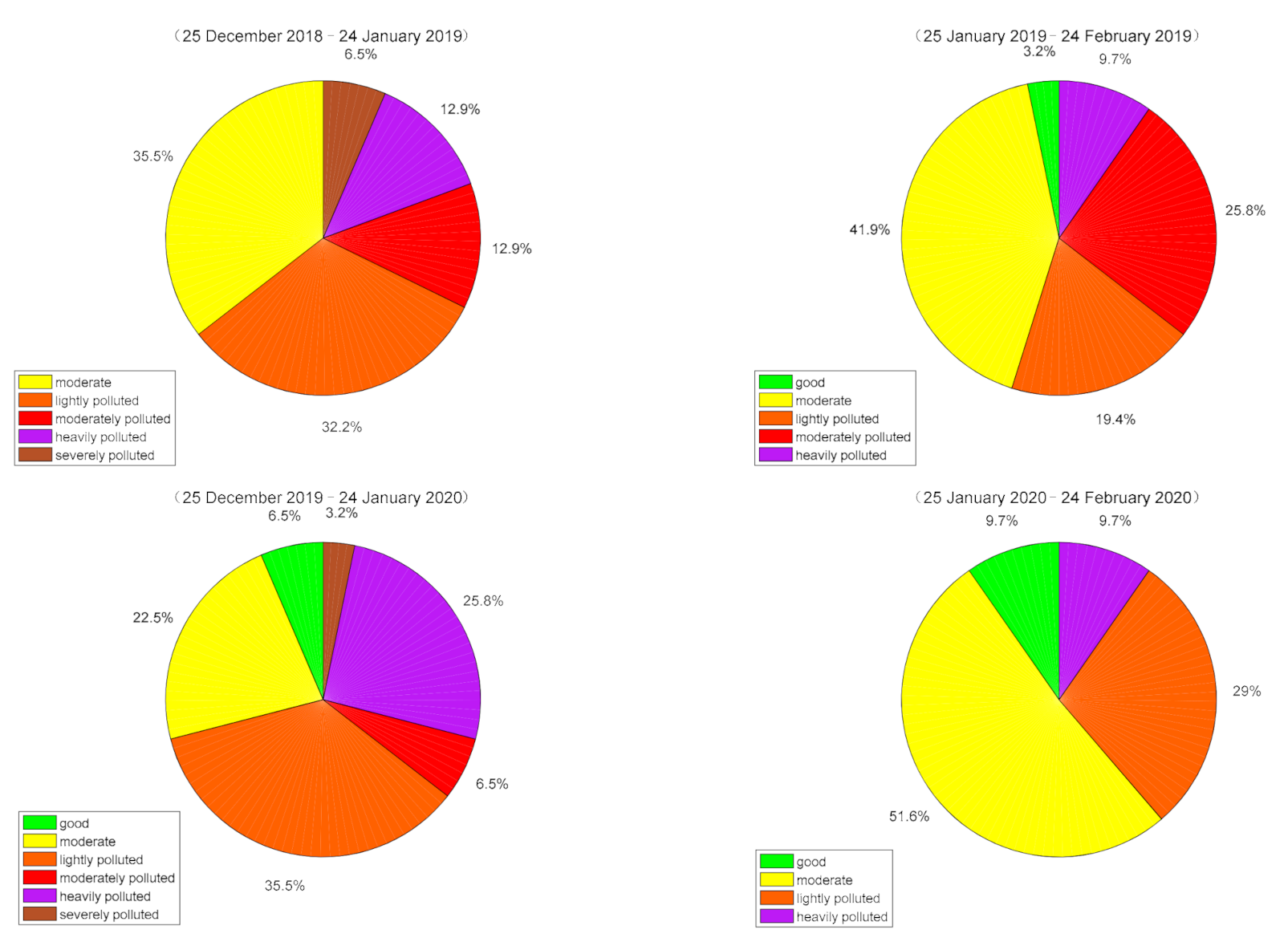
Before applying the GRA method to analyze the influence of air pollution factors on AQI, a simple numerical statistical analysis of AQI and each air pollution factor in four time periods was carried out. The four time periods mentioned here include the COVID-19 locking period (25 January 2020 to 24 February 2020), before the outbreak of COVID-19 (25 December 2019 to 24 January 2020), the same period in 2019 (25 January 2019 to 24 February 2019) and one other time period (25 December 2018 to 24 January 2019), each of which has 31 days. In addition, according to the technical regulation of ambient air quality index (AQI) (HJ 1130-2020) issued by the China Ministry of Environment of Protection, AQI can be divided into six levels (0~50 ‘good’, 51~100 ‘moderate’, 101~150 ‘lightly polluted’, 151~200 ‘moderately polluted’, 201~300 ‘heavily polluted’ and >300 ‘severely polluted’) [29]. This paper takes these as the standards to analyze the air pollution in the above four periods. The statistical results of AQI are shown in Figure 3 and

Table 1. The days of each band of AQI in different periods.

Time	Good	Moderate	Lightly Polluted	Moderately Polluted	Heavily Polluted	Severely Polluted	Total
25 December 2018–24 January 2019	0	11	10	4	4	2	31
25 January 2019–24 February 2019	1	13	6	8	3	0	31
25 December 2019–24 January 2020	2	7	11	2	8	1	31
25 January 2020–24 February 2020	3	16	9	0	3	0	31

. In the 31 days of the COVID-19 locking period (25 January 2020 to 24 February 2020), there were three days of good, 16 days of moderate, nine days of lightly polluted and three days of heavily polluted air quality, and there was no moderately polluted or severely polluted weather. In the 31 days before the outbreak of COVID-19 (25 December 2019 to 24 January 2020), respectively, and another day with severely polluted air quality the days with good and moderate grades were two and seven, respectively, the days with lightly polluted, moderately polluted and heavily polluted were 11, two and eight. In the same period of 2019 (25 January 2019 to 24 February 2019), the days of good and moderate were one and 13 respectively, the days of lightly polluted, moderately polluted and heavily polluted were six, eight and three respectively, and there was no severely polluted weather. In the fourth period (25 December 2018 to 24 January 2019), the days of good and moderate weather were zero and 11 respectively, the days of lightly polluted were 10 days, the days of moderately polluted were four days, the days of heavily polluted were four days and the days of severely polluted were two days. From these statistics, it can be seen that the air quality of the COVID-19 locking period (25 January 2020 to 24 February 2020) was significantly better than the other three periods. In fact, during the period of COVID-19 lock-in, the total number of days with good and moderate air quality was 19 days, accounting for 61.3% (19/31), and there was no severely polluted weather. However, in the other three time periods, the total number of good and moderate days of air quality were 9, 14 and 11, respectively, which did not reach 50%. In the locking period of COVID-19 (25 January 2020 to 24 February 2020), only three days reached or exceeded the moderately polluted level, accounting for 9.7% (3/31), and the other three time periods were 11 days, 11 days and 10 days, respectively, which exceeded 30%. In addition, before the outbreak of COVID-19 (25 December 2019 to 24 January 2020), and in the fourth period (25 December 2018 to 24 January 2019), there were one day and two days of severely polluted weather, respectively. All these indicate that during the period of epidemic prevention and control, the factories stopped production and motor vehicles were restricted and stopped, which played a positive role in improving air quality.

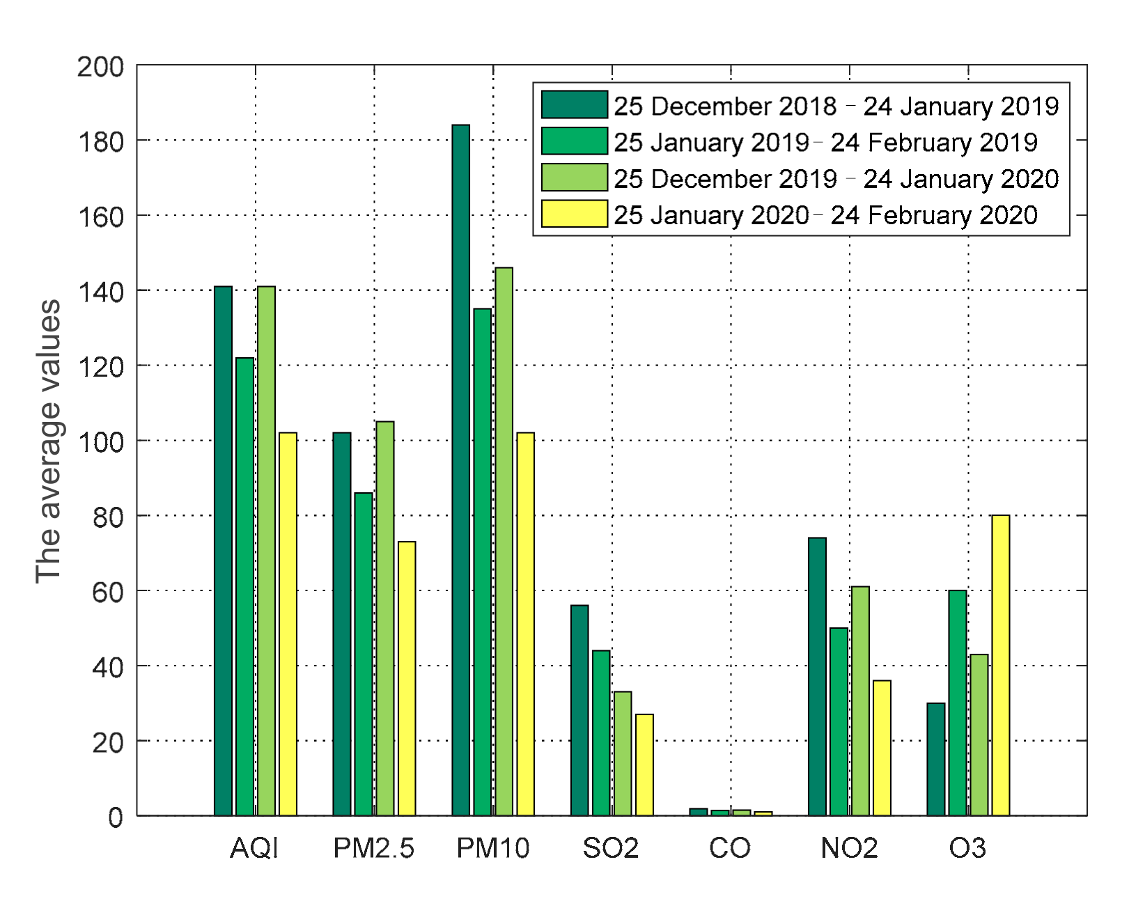
Figure 4 and

Table 2. The average values of AQI and six main pollution concentrations in different periods of time.

Time	AQI	PM2.5	PM10	SO2	CO	NO2	O3
25 December 2018–24 January 2019	141	102	184	56	1.9	74	30
25 January 2019–24 February 2019	122	86	135	44	1.4	50	60
25 December 2019–24 January 2020	141	105	146	33	1.5	61	43
25 January 2020–24 February 2020	102	73	102	27	1.0	36	80

show the average values of AQI and pollutant concentrations over the above four time periods. It can be seen that compared with the other three periods, except for the increase of the average concentration of O₃, the average value of AQI and the average concentration of other pollutants decreased significantly during the COVID-19 locking period (25 January 2020 to 24 February 2020). The average value reflects the overall level of data. Combining these results with the statistical results in Table 1 shows that the air quality in the locking period of COVID-19 was significantly better than in the other three periods. In fact, good weather accounted for 61.3% (19/31) in the COVID-19 locking period (25 January 2020 to 24 February 2020). Compared with 29% (9/31) before the outbreak of COVID-19, 45.1% (14/31) in the same period of 2019 and 35.5% (11/31) in the fourth period, there were 32.3% (10/31), 16.2% (5/31) and 25.8% (8/31) more, respectively. The number of days reaching and exceeding the moderately polluted level accounted for 9.7% (3/31), which was 25.8% (8/31), 25.8% (8/31) and 22.6% (7/31) less than that before the outbreak of COVID-19 (35.5% (11/31)) for the same period in 2019 (35.5% (11/31)) and the fourth period (32.2% (10/31)) respectively. There was no severely polluted weather during the period of COVID-19 lock-in. In addition, the average value of AQI during the locking period of COVID-19 was 102, which is smaller than the other three time periods (141, 122, 141). These results show that the prevention and control measures of COVID-19 had great restrictions on the movement of people, transportation, engineering construction, industrial production and commercial trade activities. Industrial emissions and automobile exhaust were greatly reduced, and air quality was significantly improved.

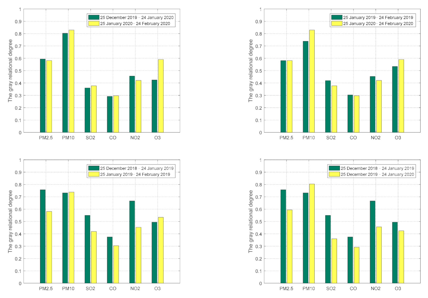
From the literature [29], we know that AQI is calculated by the concentration values of PM_2.5, PM₁₀, SO₂, CO, NO₂, O₃ and other pollutants. From previous numerical statistical analysis, we know that compared with the other three time periods the AQI and the pollution concentration changed greatly during the COVID-19 locking period. So, did the impact of these air pollutants on AQI change greatly? Next, we used the GRA method to analyze the gray relational degree of each pollution factor and AQI in the above four time periods, and made a comparative analysis of the situation in different time periods. The analysis and comparison results are shown in Figure 5 and

Table 3. The gray relational degree between pollutants and AQI between 25 December 2019 to 24 January 2020 and 25 January 2020 to 24 February 2020.

Time	PM2.5	PM10	SO2	CO	NO2	O3
25 December 2019–24 January 2020	0.5946182	0.8036469	0.3600114	0.2916706	0.456154	0.4247363
25 January 2020–24 February 2020	0.5825637	0.8290349	0.3772621	0.297143	0.4210722	0.5905432

,

Table 4. The gray relational degree between pollutants and AQI between 25 January 2019–24 February 2019 and 25 January 2020–24 February 2020.

Time	PM2.5	PM10	SO2	CO	NO2	O3
25 January 2019–24 February 2019	0.5815787	0.7384725	0.419446	0.3033536	0.453656	0.5344895
25 January 2020–24 February 2020	0.5825637	0.8290349	0.3772621	0.297143	0.4210722	0.5905432

,

Table 5. The gray relational degree between pollutants and AQI between 25 December 2018 to 24 January 2019 and 25 January 2019 to 24 February 2019.

Time	PM2.5	PM10	SO2	CO	NO2	O3
25 December 2018–24 January 2019	0.7573002	0.731805	0.5499309	0.3751351	0.6669078	0.4942023
25 January 2019–24 February 2019	0.5815787	0.7384725	0.419446	0.3033536	0.453656	0.5344895

and

Table 6. The gray relational degree between pollutants and AQI between 25 December 2018 to 24 January 2019 and 25 December 2019 to 24 January 2020.

Time	PM2.5	PM10	SO2	CO	NO2	O3
25 December 2018–24 January 2019	0.7573002	0.731805	0.5499309	0.3751351	0.6669078	0.4942023
25 December 2019–24 January 2020	0.5946182	0.8036469	0.3600114	0.2916706	0.456154	0.4247363

.

It can be seen from Table 3 and Table 4 that during the COVID-19 locking period (25 January 2020 to 24 February 2020), compared with before the outbreak of COVID-19 (25 December 2019 to 24 January 2020), the impact of PM₁₀ was slightly enhanced, the impact of PM_2.5, SO₂ and CO was basically the same as that in the earlier period, the impact of NO₂ was slightly weakened and the impact of O₃ was significantly enhanced. Compared with the same period in 2019 (25 January 2019 to 24 February 2019), the impacts of PM₁₀ and O₃ were significantly enhanced, the impacts of PM_2.5 and CO were basically the same as before and the impacts of SO₂ and NO₂ were slightly weakened.

The results in Table 5 show that in the same period of 2019 (25 January 2019 to 24 February 2019) compared with its earlier period (25 December 2018 to 24 January 2019), the impact of PM_2.5, SO₂ and NO₂ was significantly weakened, the impact of PM₁₀ was basically the same as that of the earlier period, the impact of CO was slightly weakened and the impact of O₃ was slightly enhanced. It can be seen from Table 6 that before the outbreak of COVID-19 (25 December 2019 to 24 January 2020), compared with the same period in 2018 (25 December 2018 to 24 January 2019), the impact of PM_2.5, SO₂ and NO₂ was significantly weakened, the impact of PM₁₀ was significantly enhanced and the impact of CO and O₃ was significantly enhanced.

Based on the analysis of the results in Table 3, Table 4, Table 5 and Table 6 and Figure 5, it can be seen that although there were some differences in the impact changes of pollutants on air quality (AQI) in different comparison periods, the changes were similar in the corresponding comparison periods. PM₁₀ and PM_2.5 had great influence on AQI. These results indicate that although the impact of various air pollutants on AQI had some changes due to the outbreak of COVID-19, most of the changes were not significant. Therefore, it is feasible to use the data before the outbreak of COVID-19 to predict the data during the outbreak of COVID-19, but there are also some challenges.

5.2. AQI Prediction Results and Analysis

In this part, we used five prediction models, such as ISOA-SVR, SOA-SVR, PSO-SVR, SCA-SVR and WOA-SVR, to predict the monthly average AQI values from September 2019 to June 2020, and the daily AQI values for 15–24 February 2020. In addition, in order to ensure the reliability of the experiment, each group of experiments of each model was run separately for 30 times, and the prediction results compared and analyzed.

The sampling time of Experiment 1 was from December 2013 to June 2020, with a total of 79 groups of monthly average air quality data. The first 69 groups were used as the training set and the remaining 10 groups as the test set. The sampling time of Experiment 2 was from 1 January 2020 to 24 February 2020. There were 55 groups of daily air quality data, including the first 45 groups as the training set and the remaining 10 groups as the test set. In the experiment, the AQI value of the sixth group was predicted by inputting the AQI value of the first five groups and the pollutant value of the fifth group, and then sliding forward was carried out to eliminate the random fluctuation in the historical statistical series, and to eliminate the influence of season and random factors to make more accurate predictions. The fitness convergence curve of training data and the test results of test data (including MSE, RMSE, MAPE and run time) were obtained by running each prediction model.

5.2.1. Results and Analysis of Experiment 1

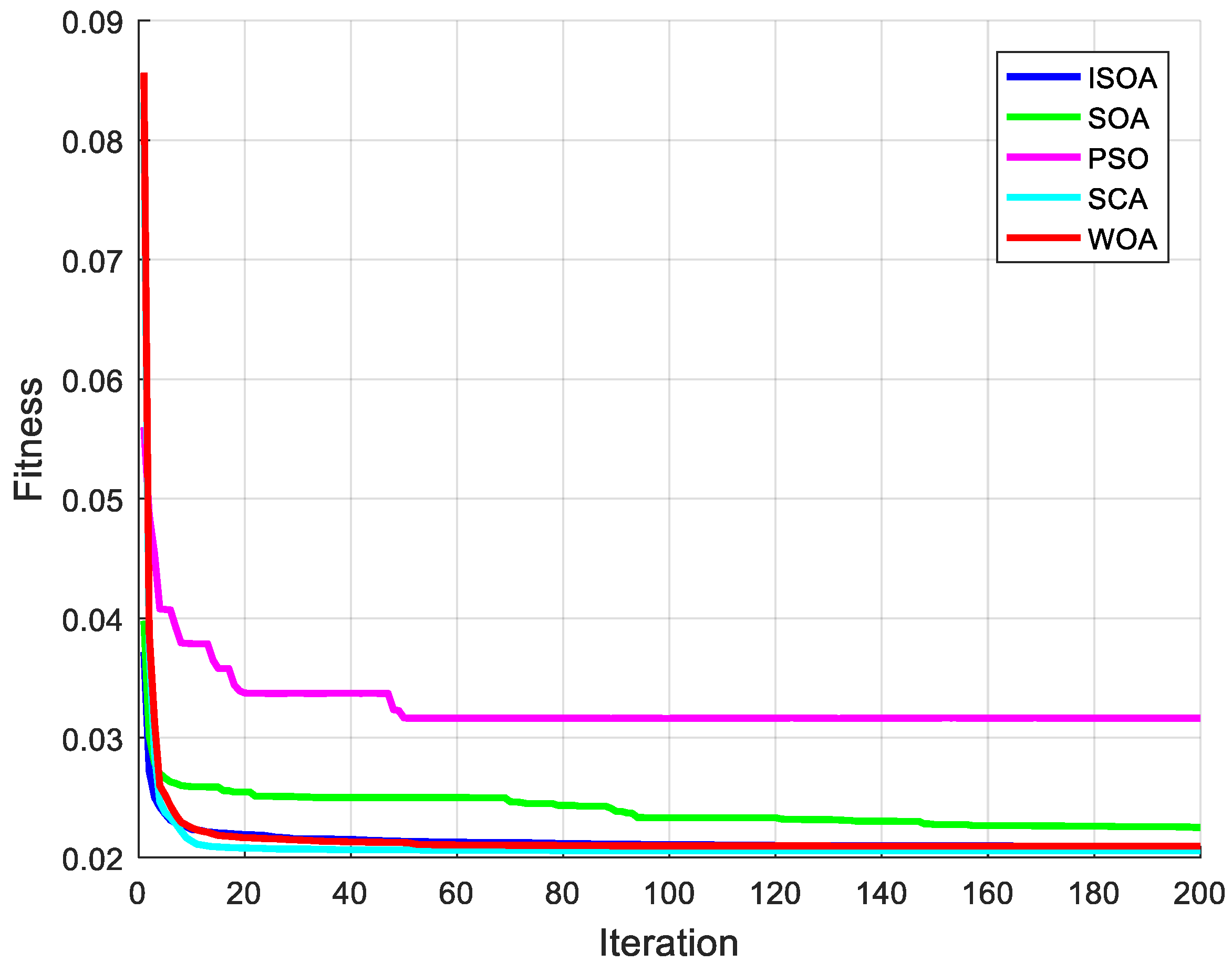
As can be seen from Figure 6, the convergence effect of fitness functions of ISOA, SCA and WOA were similar, but SOA was slightly worse, and the worst was PSO. The training results in

Table 7. The means square error (MSE), relative mean square error (RMSE) and mean percentage error (MAPE) index results of five models in Experiment 1.

	ISOA-SVR	SOA-SVR	PSO-SVR	SCA-SVR	WOA-SVR
MSE	1.299370396	1.516275653	1.783184745	1.386464339	1.367865788
RMSE	0.010565973	0.014142911	0.014833724	0.012714389	0.012364791
MAPE	9.064760441	9.853200382	9.371637923	9.62641542	9.463121198

show that ISOA-SVR was the best, MSE, RMSE and MAPE were 1.299370396, 0.010565973 and 9.064760441, SCA-SVR was 1.386464339, 0.012714389 and 9.62641542, and WOA-SVR were 1.367865788, 0.012364791 and 9.463121198, respectively. From the evaluation index values of the prediction results in

Table 8. The results of MSE, RMSE and MAPE of five models in Experiment 1.

	ISOA-SVR	SOA-SVR	PSO-SVR	SCA-SVR	WOA-SVR
MSE	3.379206115	3.441986222	4.349283613	3.498150956	3.41400161
RMSE	0.03090546	0.03230673	0.038231575	0.030672679	0.031900138
MAPE	14.03810752	15.60277275	18.02718993	14.65850732	14.31309124

, we found that the three index values of the prediction results of ISOA-SVR were the best, which were 3.379206115, 0.03090546 and 14.03810752, respectively. WOA-SVR was slightly worse than the ISOA-SVR algorithm, SOA-SVR and SCA-SVR were similar, both slightly lower than WOA-SVR, and PSO-SVR was the worst. In fact, we found from the prediction results in

Table 9. The predicted value of the monthly average AQI index of Taiyuan in 10 months (September 2019 to June 2020) by five models.

Months	Actual	ISOA-SVR	SOA-SVR	PSO-SVR	SCA-SVR	WOA-SVR
September 2019	80	82.77198055	85.5977246	88.28627583	84.48194106	82.38016393
October 2019	86	91.75390427	92.79561765	104.4254211	95.03535344	91.52332133
November 2019	102	108.1564331	107.1279498	113.0787421	109.4848466	108.7885621
December 2019	95	129.8122227	124.8458292	120.8050922	129.2580647	130.9492776
January 2020	153	120.1545213	119.9753754	109.4081433	118.2433733	120.5372071
February 2020	108	128.1305829	127.0634554	127.8660077	128.9146531	127.4201454
March 2020	77	95.40056339	99.44739009	92.53519639	93.96113427	95.63228132
April 2020	83	94.20694095	95.92648075	101.5208532	89.12996596	95.75164039
May 2020	88	88.36159652	94.17246856	104.1960515	83.85785511	90.30725226
June 2020	123	111.1573034	106.1393318	119.698614	109.623607	113.3392755

that the prediction result of ISOA-SVR achieved the optimal value or suboptimal value in 6/10, which was the best among the five algorithms.

5.2.2. Results and Analysis of Experiment 2

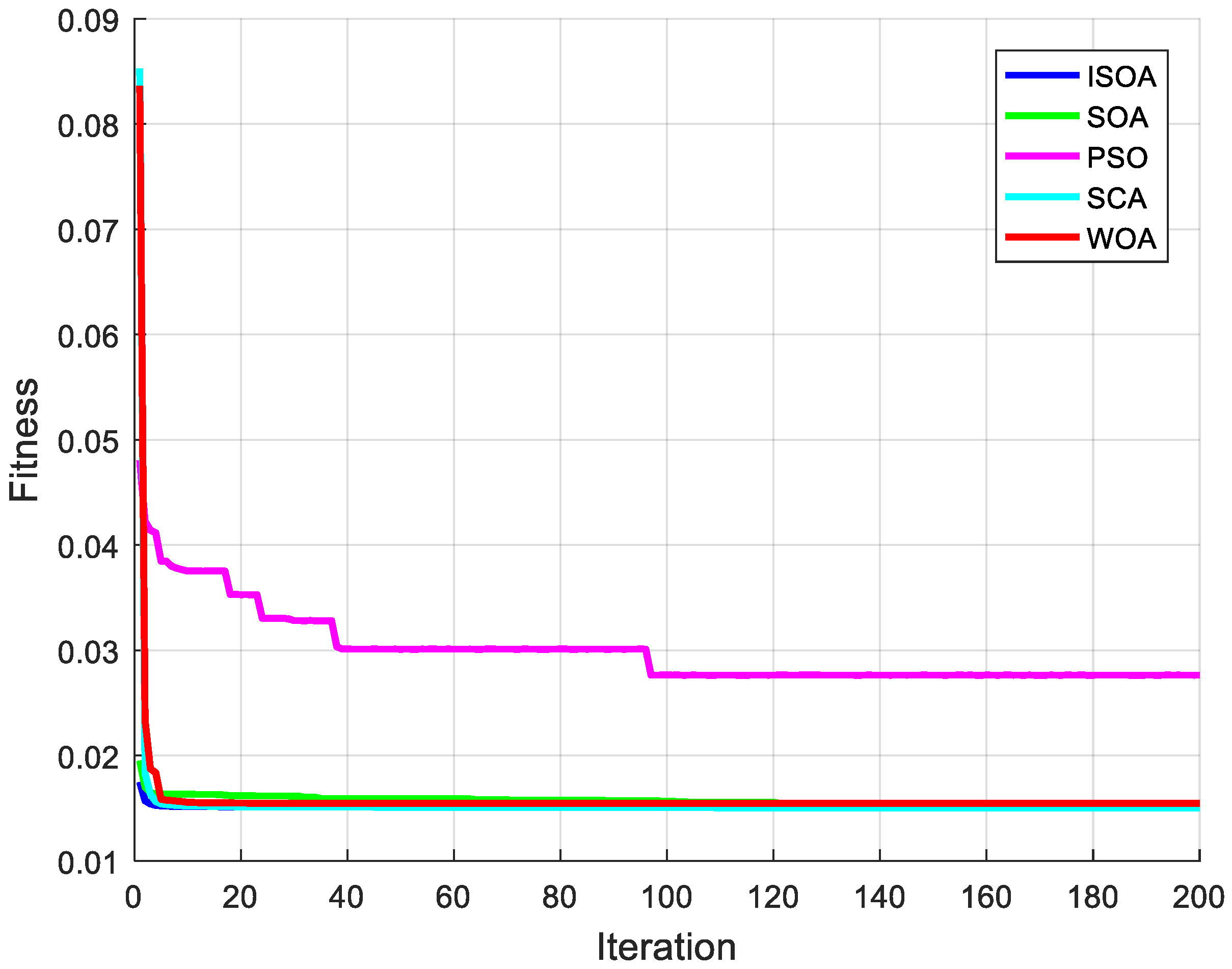
We can see from Figure 7 that the convergence effect of fitness function of ISOA, SOA, SCA and WOA were similar, but the convergence effect of PSO was a little worse. From the MSE, RMSE and MAPE of the training results in

Table 10. The MSE, RMSE and MAPE index results of five models in Experiment 2.

	ISOA-SVR	SOA-SVR	PSO-SVR	SCA-SVR	WOA-SVR
MSE	13.37973604	12.90917741	15.26069105	13.38228635	13.67762998
RMSE	0.163687428	0.162034198	0.263342202	0.164932562	0.176975593
MAPE	28.1740733	28.71513087	36.06950441	28.34307946	30.06256388

, we found that the training results of ISOA-SVR (13.37973604, 0.163687428 and 28.1740733) were slightly worse than the best SOA-SVR (12.90917741, 0.162034198 and 28.71513087), but better than other algorithms. From the three evaluation index values of the prediction results in

Table 11. The results of MSE, RMSE and MAPE of five models in Experiment 2.

	ISOA-SVR	SOA-SVR	PSO-SVR	SCA-SVR	WOA-SVR
MSE	6.147418336	6.459778601	10.82499818	6.689566261	7.5729638
RMSE	0.185148465	0.185470358	0.416901153	0.201263888	0.259079722
MAPE	37.28176518	37.73182296	53.0989463	39.01383564	43.56969294

, we can see that the prediction results of ISOA-SVR were the best (6.147418336, 0.185148465 and 37.28176518), SOA-SVR was slightly worse than the ISOA-SVR algorithm, SCA-SVR was better than WOA-SVR and was slightly lower than SOA-SVR; the worst was PSO-SVR. In fact, from the prediction results in

Table 12. The predicted value of the monthly average AQI index of Taiyuan in 10 days (15 February 2020 to 24 February 2020) by five models.

Days	Actual	ISOA-SVR	SOA-SVR	PSO-SVR	SCA-SVR	WOA-SVR
15 February 2020	37	66.19915498	64.1716092	81.11185736	66.77559426	68.29006364
16 February 2020	40	63.56384349	63.11114188	78.85186159	64.56873662	73.61728757
17 February 2020	50	64.31550156	65.53302046	77.72392869	66.30127468	73.6344107
18 February 2020	64	83.45317703	85.22290481	94.48414881	86.02403533	92.64726525
19 February 2020	77	98.39158683	101.4637515	107.20132	101.8584487	104.1777717
20 February 2020	107	102.5547977	104.7637718	113.8703628	104.7694695	104.8558503
21 February 2020	67	109.1720281	111.3754232	122.0536657	110.3169339	109.5317368
22 February 2020	56	76.30078067	76.27921803	92.07265008	76.87427183	77.86190836
23 February 2020	99	77.99825975	77.10175492	93.3506996	78.34032184	85.4347774
24 February 2020	137	104.6398589	104.8715531	118.3346012	104.0343253	107.4976793

, we found that the prediction result of ISOA-SVR achieved the optimal value or suboptimal value in 7/10, which was the best among the five algorithms.

Combined with the results of Experiment 1 and Experiment 2, we can conclude that the proposed ISOA-SVR prediction model had better generalization ability and robustness than other prediction models tested in this study. This good result is attributed to the three characteristics of the ISOA algorithm: one is the exponential balance of local and global optimization; the second is the adaptive ability of particles themselves and groups and the third is the diversity of particles. These make the algorithm avoid falling into local minimums in the process of optimization. In addition, the weight parameters introduced in the ISOA algorithm can balance the global exploration and local development ability of particles and accelerate the convergence speed of the algorithm.

6. Conclusions

This study focused on air quality evaluation during the COVID-19 lock down (25 January 2020 to 24 February 2020), before the COVID-19 outbreak (25 December 2019 to 24 January 2020), the same period in 2019 (25 January 2019 to 24 February 2019) and another time period (25 December 2018 to 24 January 2019). First, a numerical statistics comparative analysis was made, and then the grey relational analysis (GRA) method was used to analyze the relational degree between six major pollutants and AQI. The results not only reflect the distribution of air quality index (AQI) and pollutant concentration in each analysis period, but also reflect the impact of pollutants on AQI. The air condition during the locking period of COVID-19 was evaluated. The results show that during the locking period of COVID-19, the overall air condition was good, good and moderate weather accounted for a large proportion of the period, and there was no severely polluted weather. The average air quality index (AQI) and the average concentrations of five pollutants except O₃ decreased significantly. PM₁₀ was still the main factor affecting AQI. This indicates that air pollution was closely related to the higher pollutant discharge. The prevention and control measures during the COVID-19 locking period reduced the emissions of industrial waste gas, automobile exhaust and other pollutants in Taiyuan. Taiyuan greatly improved its air. However, coal-fired heating in winter still contributes a lot to PM₁₀ concentration. In addition, the evaluation results also reflect that the average concentration of O₃ increased slightly during the period of prevention and control of COVID-19, which deserves our attention.

After the evaluation of air quality, this study constructed an ISOA-SVR prediction model for the prediction of AQI value of air quality. Air quality is affected by many factors such as pollution sources and the meteorological environment, which makes AQI prediction inaccurate and difficult. SVR is suitable for AQI prediction, but its prediction effect depends on the selection of model parameters. First, based on the SOA algorithm, this study proposed the ISOA algorithm by introducing nonlinear parameters, considering the influence of individual extreme and average adaptations of each generation, and increasing the diversity of particles. Then, the parameters of the SVR model were optimized by the ISOA algorithm. Finally, the optimized ISOA-SVR prediction model was used to analyze the monthly average AQI values from September 2019 to June 2020, and the daily AQI values for 15–24 February 2020, respectively. The results were compared with those of the SVR prediction models optimized by the SOA, PSO, SCA and WOA algorithms. Finally, the results showed that the SVR model optimized by the ISOA algorithm achieved good results in MSE, RMSE and MAPE.

To sum up, first of all, the air quality evaluation results of Taiyuan in this study were in line with the air quality situation of Taiyuan city. Secondly, the integrated prediction model of ISOA-SVR proposed in this study was suitable for the prediction of AQI value of air quality in Taiyuan before and after COVID-19 epidemic. These results can play a guiding role in the prevention and control of air quality in Taiyuan and other places.

References

- Guan, W.-J.; Zheng, X.-Y.; Chung, K.F.; Zhong, N.-S. Impact of air pollution on the burden of chronic respiratory diseases in China: Time for urgent action. Lancet 2016, 388, 1939–1951. [Google Scholar] [CrossRef]
- Trenton Straube. Top 10 Threats to Global Health in 2019. 13 February 2019. Available online: https://www.poz.com/article/top-10-threats-global-health-2019 (accessed on 6 January 2021).
- Kyrkilis, G.; Chaloulakou, A.; Kassomenos, P.A. Development of an aggregate air quality index for an urban Mediterranean agglomeration: Relation to potential health effects. Environ. Int. 2007, 33, 670–676. [Google Scholar] [CrossRef]
- China Ministry of Environmental Protection. Ambient Air Quality Standards; GB 3095–2012; China Environmental Science Press: Beijing, China, 2012.
- Siew, L.Y.; Chin, L.Y.; Mah, P.; Wee, J. Arima and integrated Arfima models for forecasting air pollution index in shah alam, Selangor. Malays. J. Anal. Sci. 2008, 12, 257–263. [Google Scholar]
- Zhu, J.; Zhang, R.; Fu, B.; Jin, R. Comparison of ARIMA model and exponential smoothing model on 2014 air quality index in yanqing county, Beijing, China. Appl. Comput. Math. 2015, 4, 456. [Google Scholar] [CrossRef] [Green Version]
- Drucker, H.; Burges, C.J.; Kaufman, L.; Smola, A.; Vapnik, V. Support vector regression machines. Adv. Neural Inf. Process. Syst. 1997, 28, 779–784. [Google Scholar]
- Basak, D.; Pal, S.; Patranabis, D.C. Support vector regression. Neural Inf. Process. Lett. Rev. 2007, 11, 203–224. [Google Scholar]
- Chen, S.-T.; Yu, P.-S.; Tang, Y.-H. Statistical downscaling of daily precipitation using support vector machines and multivariate analysis. J. Hydrol. 2010, 385, 13–22. [Google Scholar] [CrossRef]
- Kavousi-Fard, A.; Kavousi-Fard, F. A new hybrid correction method for short-term load forecasting based on ARIMA, SVR and CSA. J. Exp. Theor. Artif. Intell. 2013, 25, 559–574. [Google Scholar] [CrossRef]
- Chen, Y.; Xu, P.; Chu, Y.; Li, W.; Wu, Y.; Ni, L.; Bao, Y.; Wang, K. Short-term electrical load forecasting using the Support Vector Regression (SVR) model to calculate the demand response baseline for office buildings. Appl. Energy 2017, 195, 659–670. [Google Scholar] [CrossRef]
- Liu, H.; Li, Q.; Yu, D.; Yu, G. Air quality index and air pollutant concentration prediction based on machine learning algo-rithms. Appl. Sci. 2019, 9, 4069. [Google Scholar] [CrossRef] [Green Version]
- Castelli, M.; Clemente, F.M.; Popovič, A.; Silva, S.; Vanneschi, L. A machine learning approach to predict air quality in California. Complexity 2020, 2020, 1–23. [Google Scholar] [CrossRef]
- Dun, M.; Xu, Z.; Chen, Y.; Wu, L. Short-term air quality prediction based on fractional grey linear regression and support vector machine. Math. Probl. Eng. 2020, 2020, 1–13. [Google Scholar] [CrossRef]
- Chen, K.-Y.; Wang, C.-H. Support vector regression with genetic algorithms in forecasting tourism demand. Tour. Manag. 2007, 28, 215–226. [Google Scholar] [CrossRef]
- Wu, C.-H.; Tzeng, G.-H.; Lin, R.-H. A novel hybrid genetic algorithm for kernel function and parameter optimization in support vector regression. Expert Syst. Appl. 2009, 36, 4725–4735. [Google Scholar] [CrossRef]
- Wang, J.; Li, L.; Niu, D.; Tan, Z. An annual load forecasting model based on support vector regression with differential evolution algorithm. Appl. Energy 2012, 94, 65–70. [Google Scholar] [CrossRef]
- Zhang, F.; Deb, C.; Lee, S.E.; Yang, J.; Shah, K.W. Time series forecasting for building energy consumption using weighted support vector regression with differential evolution optimization technique. Energy Build. 2016, 126, 94–103. [Google Scholar] [CrossRef]
- Hong, W.-C. Chaotic particle swarm optimization algorithm in a support vector regression electric load forecasting model. Energy Convers. Manag. 2009, 50, 105–117. [Google Scholar] [CrossRef]
- Duan, P.; Xie, K.; Guo, T.; Huang, X. Short-term load forecasting for electric power systems using the PSO-SVR and FCM clustering techniques. Energies 2011, 4, 173–184. [Google Scholar] [CrossRef] [Green Version]
- Bui, X.-N.; Lee, C.W.; Nguyen, H.; Bui, H.-B.; Long, N.Q.; Le, Q.-T.; Nguyen, V.-D.; Nguyen, N.-B.; Moayedi, H. Estimating PM10 concentration from drilling operations in open-pit mines using an assembly of SVR and PSO. Appl. Sci. 2019, 9, 2806. [Google Scholar] [CrossRef] [Green Version]
- Cao, G.; Wu, H. Support vector regression with fruit fly optimization algorithm for seasonal electricity consumption forecasting. Energy 2016, 115, 734–745. [Google Scholar] [CrossRef]
- Xu, C.; Amar, M.N.; Ghriga, M.A. Evolving support vector regression using grey wolf optimization; forecasting the geome-chanically properties of rock. Eng. Comput. 2020, 2020, 1–15. [Google Scholar]
- Deng, J.L. Introduction to grey system theory. J. Grey Syst. 1989, 1, 1–24. [Google Scholar]
- Dhiman, G.; Kumar, V. Seagull optimization algorithm: Theory and its applications for large-scale industrial engineering problems. Knowl. Based Syst. 2019, 165, 169–196. [Google Scholar] [CrossRef]
- Eberhart, R.C.; Kennedy, J. A new optimizer using particle swarm theory. In Proceedings of the 6th International Symposium on Micro Machine and Human Science, Nagoya, Japan, 4–6 October 1995; Volume 1, pp. 39–43. [Google Scholar]
- Mirjalili, S. SCA: A sine cosine algorithm for solving optimization problems. Knowl. Based Syst. 2016, 96, 120–133. [Google Scholar] [CrossRef]
- Mirjalili, S.; Lewis, A. The whale optimization algorithm. Adv. Eng. Softw. 2016, 95, 51–67. [Google Scholar] [CrossRef]
- China Ministry of Environmental Protection. Technical Regulation on Ambient Air Quality Index (AQI); HJ 633–2012; China Environmental Science Press: Beijing, China, 2012.
Figure 1.
A schematic diagram of support vector regression (SVR).
Figure 2.
Migration and attack pattern of seagulls.
Figure 3.
The proportion of days in each band of air quality index (AQI) in different periods.
Figure 4.
The average values of AQI and six main pollution concentrations in different periods of time.
Figure 5.
Comparison of the gray relational degree between pollutants and AQI in different periods of time.
Figure 6.
Fitness convergence curves of five algorithms in Experiment 1.
Figure 7.
Fitness convergence curves of five algorithms in Experiment 2.