
Modeling the COVID-19 Pandemic Dynamics in Egypt and Saudi Arabia


1
Management Information System Department, Yanbu, Taibah University, Yanbu 46421, Saudi Arabia
2
Department of Statistics, Mathematics and Insurance, Benha University, Benha 13513, Egypt
3
College of Computer Science and Engineering, Taibah University, Yanbu 46421, Saudi Arabia
4
Department of Applied Statistics, Faculty of Graduate Studies for Statistical Research, Cairo University, Giza 12613, Egypt
*
Author to whom correspondence should be addressed.
Mathematics 2021, 9(8), 827; https://doi.org/10.3390/math9080827
Submission received: 4 March 2021
/
Revised: 27 March 2021
/
Accepted: 7 April 2021
/
Published: 10 April 2021
(This article belongs to the Special Issue Statistical Methods for the Analysis of Infectious Diseases)
Abstract
:During the abrupt outbreak of the COVID-19 pandemic, the public health system of most of the world’s nations has been tested. However, it is the concern of governments and other responsible entities to provide the correct statistics and figures to take any practicable necessary steps such as allocation of the requisite quarantine operations, calculation of the needed number of places in hospitals, determination of the extent of personal security, and determining the degree of isolation of infectious people, among others. Where the statistical literature supposes that a model governs every real phenomenon, once we know the model, we can evaluate the dilemma. Therefore, in this article, we compare the COVID-19 pandemic dynamics of two neighboring Arabic countries, Egypt and Saudi Arabia, to provide a framework to arrange appropriate quarantine activities. A new generalized family of distributions is developed to provide the best description of COVID-19 daily cases and data on daily deaths in Egypt and Saudi Arabia. Some of the mathematical properties of the proposed family are studied.
1. Introduction
In the past few months, the COVID-19 pandemic has dominated the world and the international health community. Many authors have made efforts to compare the epidemic patterns of various regions. Nesteruk [1] provided a q the epidemic dynamics in Italy and mainland China [2] and provided a comparison of the epidemic dynamics in Ukraine and neighboring countries [3]. Zhao et al. [4] compared the COVID-19 pandemic dynamics of two neighboring Asian countries, Iran and Pakistan, and developed a new statistical model describing data on COVID-19 daily deaths in Iran and Pakistan. There have been some efforts to try to model the dynamics of the disease, such as by Zhao et al. [4] Sarkodie and Owusu [5], Giordano et al. [6], Anastassopoulou et al. [7], Naik et al. [8], Musa et al. [9], Alghamdi et al. [10], and Langemann et al. [11]. There have also been several efforts to use machine learning to model disease dynamics. La Gatta et al. [12] looked at using deep learning for epidemiological research and for learning about Covid19 spatio-temporal patterns. Nadler et al. [13] applied a neural susceptible-infected-recovered (SIR) model to developed and developing countries forecast confirmed infections, and analyzed future trajectories.
In the statistical literature, suppose that a model governs every real phenomenon. Once we know the model, we can fully evaluate our dilemma or phenomenon. Several different approaches have been created to build new models from older ones, and several continuous distributions were constructed by expanding other common continuous distributions; see, for example, Alzaatreh and Famoye [14], Al-Babtain et al. [15], Jayakumar and Mathew [16], Cordeiro et al. [17], Oluyede et al. [18], Mansour and Mahdy [19], Maurya et al. [20], Abouammoh and Kayid [21], Chen [22], Mansour et al. [23] and Tahir et al. [24].
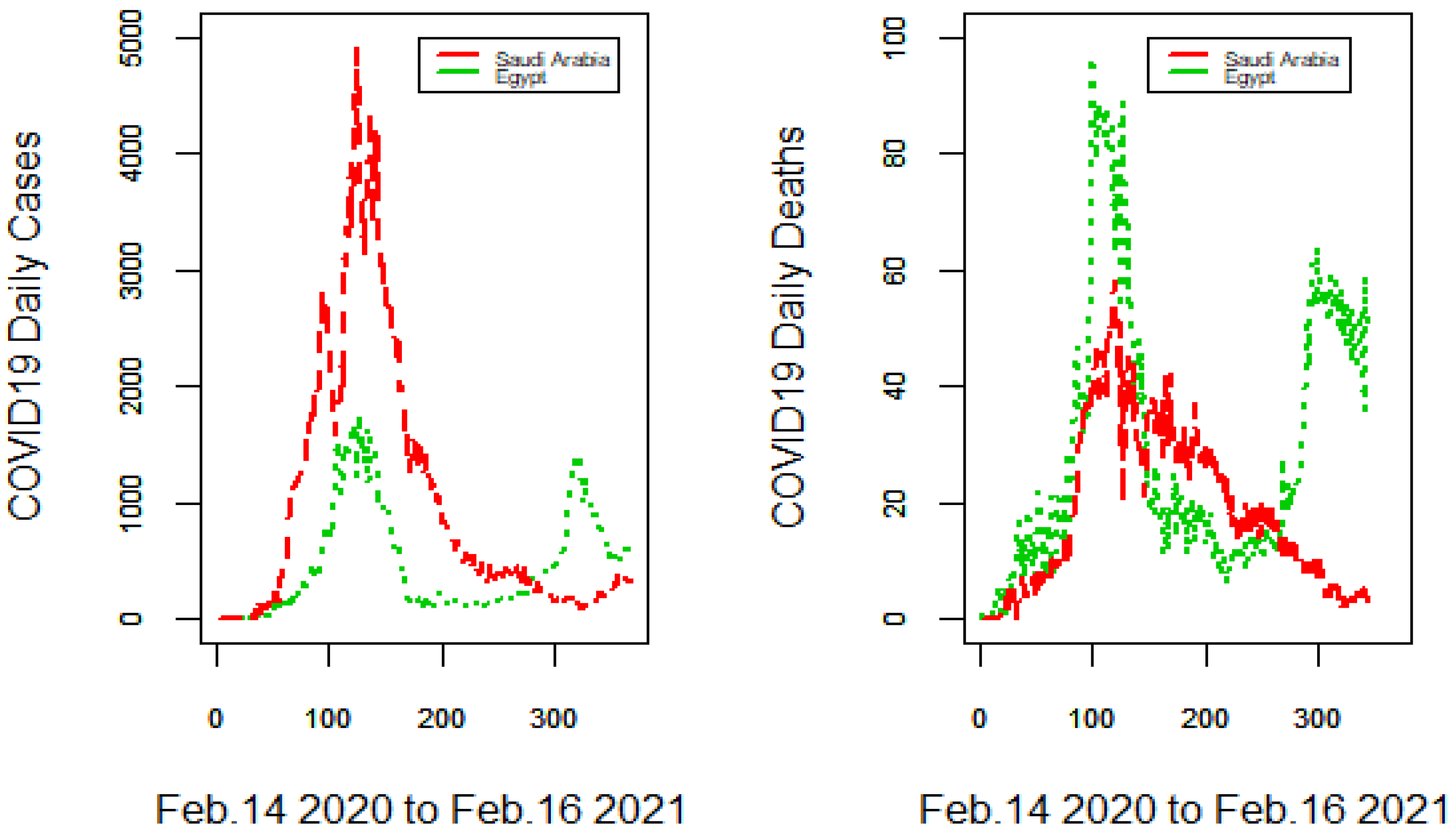
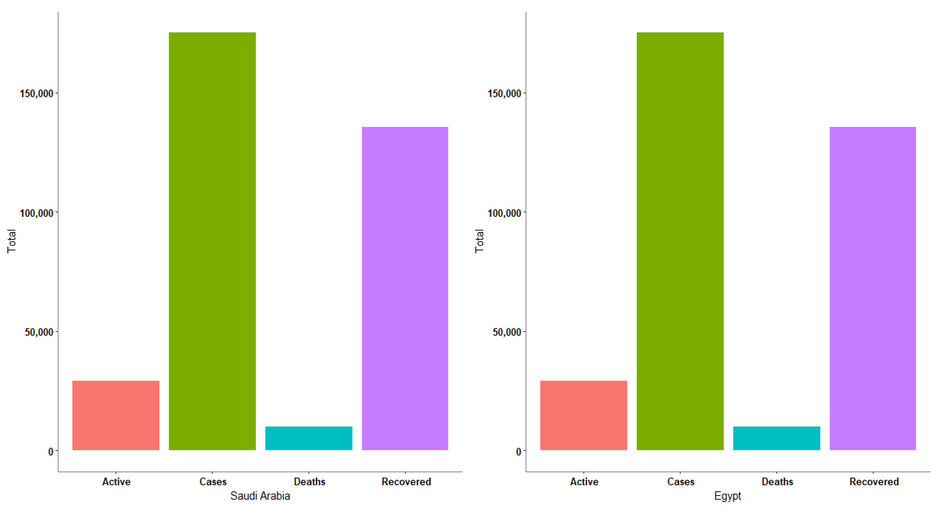
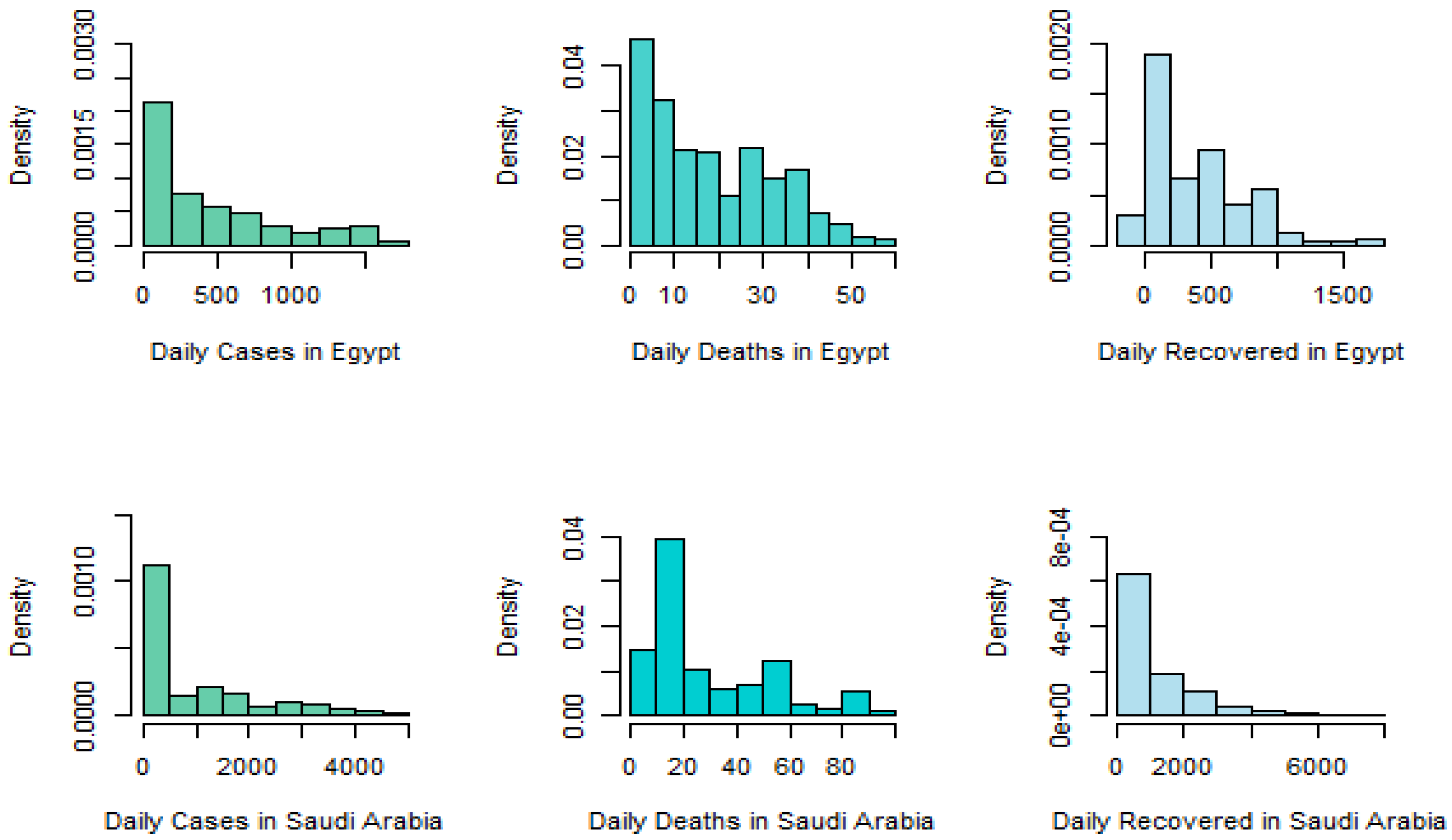
Here, we present a fundamental study to compare Saudi Arabia’s and Egypt’s outbreak dynamics, which reports the total number of outbreaks, full recoveries, total fatalities, and real active cases. COVID-19 daily cases and daily deaths in Egypt and Saudi Arabia are presented in Figure 1. From Figure 1, it is obvious that the number of daily cases in Saudi Arabia is more than the number of daily cases in Egypt, but the number of daily deaths in Saudi Arabia is less than the number of daily deaths in Egypt. Additionally, the total number of cases, total number recovered, the total number of deaths, and the total number of active cases are all found in Figure 2. The histogram for COVID-19 daily cases, daily deaths, and daily recovered in Egypt and Saudi Arabia is displayed in Figure 3. It is clear that the shapes of the distributions differ for different data. There is much interest in creating more flexible statistical distributions to describe real-world phenomena in the statistics field. Many different types of generalized distributions have been developed and applied to various phenomena. The fact that these generalized distributions have more parameters is a common feature. After looking at the existing generalized distributions, and the shapes of the distributions in Figure 3, we found that we need a new generalized family of distributions to provide an adequate description of COVID-19 daily cases and daily death data in Egypt and Saudi Arabia.
This article is structured as follows: the proposed method is discussed in Section 2. Section 3 presents the estimation of the model parameters. A special case of the proposed method is introduced in Section 4. Some properties of the proposed method are discussed in Section 5. Section 6 is devoted to modeling COVID-19 events. Finally, the article is concluded in the last section.
2. Proposed Family
In the statistical literature, we suppose that some models govern every real phenomenon. Once we know the model, we can fully evaluate our dilemma or phenomenon, since different models have been built to accomplish this mission. Poisson distribution is one of the most famous models that also provides a family of distribution. Using that family, several lifetime models have been proposed and their properties studied by several authors (see Maurya and Nadarajah [25]). Nadarajah and Cancho [26] proposed a three-parameter geometric exponential Poisson distribution, which is a compound distribution of a geometric exponential model with zero truncated Poisson distribution. This depended on the principle (minimum and maximum) used in series and parallel structures. In this section, we present a new generalized geometric Poisson (NGGP) family. This depends on the principle (maximum and minimum) used in parallel and series structures. The cumulative distribution function (cdf) of the NGGP family of distributions is defined by
where is a baseline cdf which depends on parameter vector . The corresponding probability density function, hazard rate function and reversed failure rate function are
where is a baseline pdf which depends on parameter vector ,
and
The shapes of (2) and (3) can be studied by taking their derivatives. Note that
and
The quantile function corresponding to (1) is
Using the series expansion, we can express (1) and (2) as mixtures.
We can rewrite as
and
3. Maximum Likelihood Estimation
In this section, to achieve estimates of the maximum likelihood estimators (MLEs) of the parameters of the NGGP family, we draw full samples from the population. Let be the observed sample from Equation (2). The log-likelihood function can be represented as
The partial derivatives of the log-likelihood function for the parameters are given, respectively by
and
The maximum likelihood estimator of is obtained by solving the nonlinear system of Equations (6)–(8). It is usually more convenient to use nonlinear optimization algorithms such as the quasi-Newton algorithm to numerically maximize the log-likelihood function.
4. A Special Sub Model
Nadarajah and Haghighi [27] proposed a generalization of the exponential distribution, called Nadarajah-Haghighi (NH) distribution, with density and distribution functions given by
and
respectively.
By using (1), (2), (9) and (10), the cdf and probability density function (pdf) of the new geometric Nadarajah-Haghighi Poisson (NGNHP) distribution are given by
and
respectively.
5. Statistical Properties
In this section, we derive computable representations for some statistical functions associated with the NGNHP distribution, whose pdf admits a simple representation.
5.1. Expansion for the NGNHP Density Function
An expansion for Equation (11) can be derived using (5), (9), and (10). We also consider the following expansions:
Then, the NGNHP pdf can be expressed as
where
5.2. Moments
The most important properties of a distribution can be studied by studying the moments of the distribution. The rth ordinary moment of the NGNHP, say , using Equation (13) is given by:
By noting that , we can write
where
for and setting we have
and then, after some algebra, we can write
The most general case of the binomial theorem is the identity
where is a binomial coefficient and is a real number. This power series converges when is an integer or . By using (16) in Equation (15), since , it follows by interchanging the sum and the integral that
Then, we can write from (14)
Next, we find a lemma.
Lemma 1.
The rth incomplete moment of X, sayis given by
where . Then we have
Proof.
The proof follows easily by changing variables in the integration.
The first incomplete moment of X, denoted by , is computed by taking a given value of r = 1. The first incomplete moment is significant in the calculation of various statistics and the Bonferroni and Lorenz curves. The degree of variability in a population is calculated by calculating the frequency of the individual differences from the mean and the median. The mean deviations, about the mean and about the median of X, depend on . □
6. Modeling COVID-19 Daily Cases and Daily Deaths in Egypt and Saudi Arabia
As we mentioned above, more statistical analysis of COVID-19 events is needed before any conclusions can be made. However, it is now required to formulate a fitting model to classify COVID-19 incidents, such as daily cases, total cases, daily deaths, total deaths, etc., to obtain a good estimate of the quarantine activities.
In this section, we model COVID-19 daily cases and daily deaths data in Egypt and Saudi Arabia from 14 February 2020 to 16 February 2021. The proposed NGNHP distribution is applied to this data, and the proposed NGNHP model can be applied effectively to provide the best description of COVID-19 daily cases and daily deaths data of the two neighbor countries.
To compare with other distributions in order to know which distribution provides the best fits to data, we consider specific discrimination measures such as Akaike information criterion (AIC), Corrected Akaike Information Criterion (CAIC), and Bayesian information criterion (BIC). It is well established that choosing the right approximation model to align accuracy with the alternatives is preferred. It is necessary to assess the distributional parameters of a parametric model since the distribution of these parameters will dramatically affect the overall fit’s adequacy. The maximum likelihood estimates of the model parameters for Egyptian COVID-19s daily cases data, Saudi COVID-19 daily cases data, Egyptian COVID-19 daily deaths data and Saudi COVID-19 daily deaths data are provided in Table 1. The discrimination measures for Egyptian COVID-19 daily cases data, Saudi COVID-19 daily cases data, Egyptian COVID-19 daily deaths data and Saudi COVID-19 daily deaths data are presented in Table 2.
Distribution fitting helps us create accurate models of the random processes we operate with, saving us from time and money losses caused by incorrect model selection and leading to smarter business decisions. Parameters define distributions. The maximum likelihood estimation method is used to estimate the distribution’s parameters from a data set. There are many methods for checking how “good” the distribution matches the data. Comparing the histogram to the probability density function, comparing the empirical distribution function to the underlying cumulative distribution function, constructing a Q–Q (quantile–quantile) plot, which is a graphical method for comparing two probability distributions by plotting their quantiles against each other, and constructing a P-P plot are all examples of goodness of fit methods.
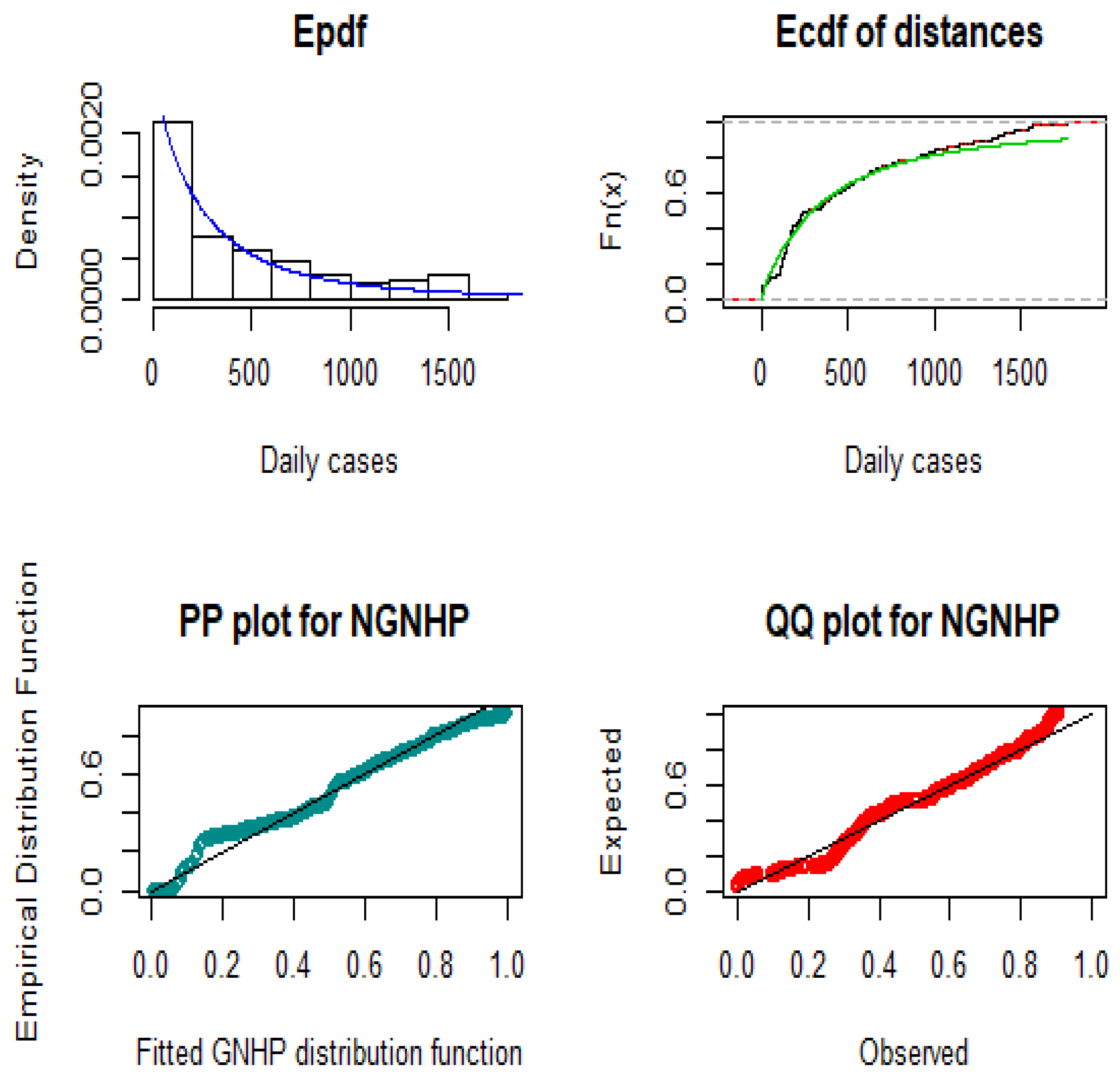
Thus, after computing the model parameters’ values, we can now show how the proposed model provides the best description of COVID-19 daily cases data and COVID-19 daily deaths data. For such a purpose, we considered the graphical sketching of the estimated pdf (Epdf), the estimated cdf (Ecdf), the probability–probability (PP) plot, and the quantile–quantile (QQ) plot.
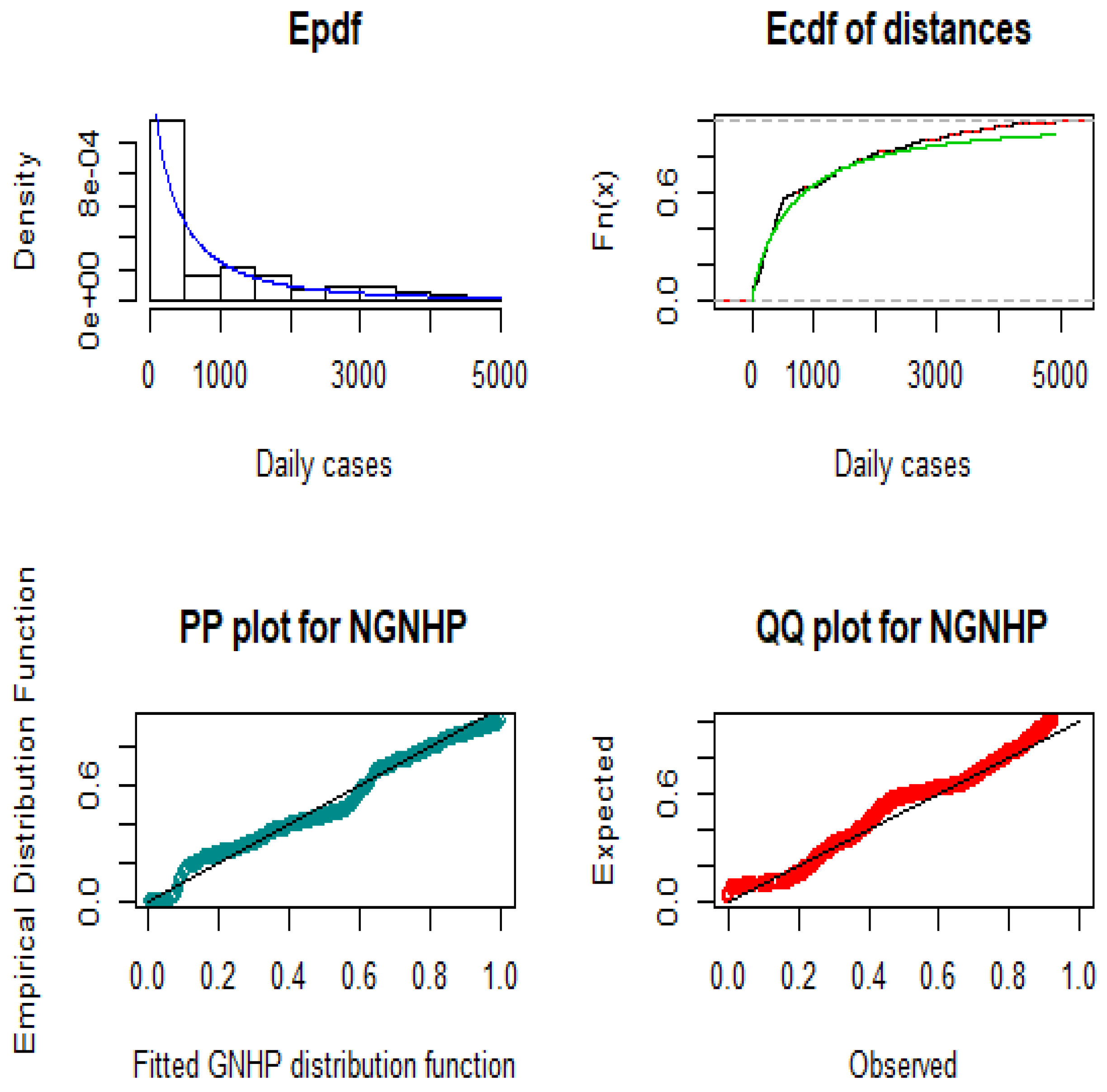
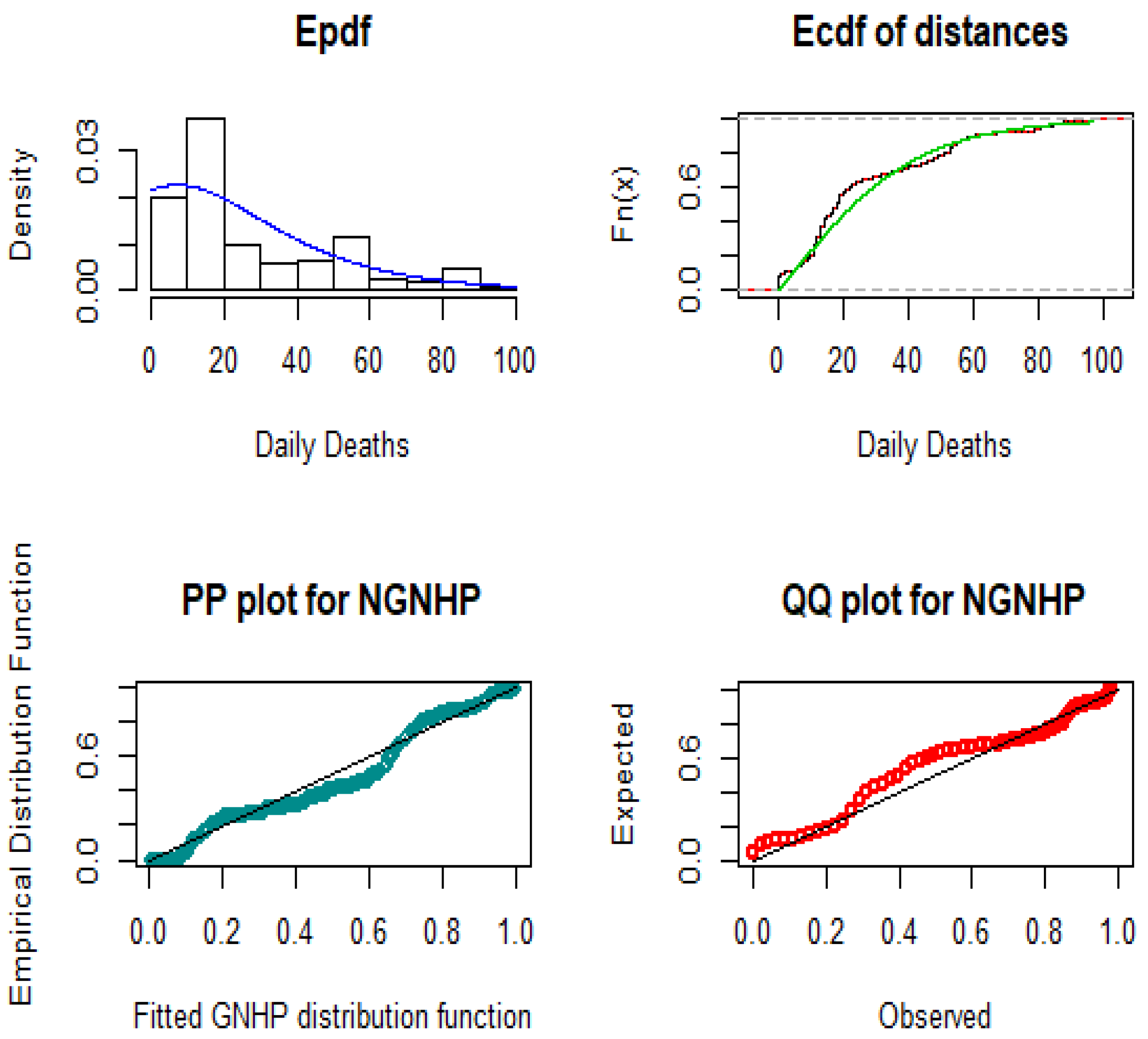
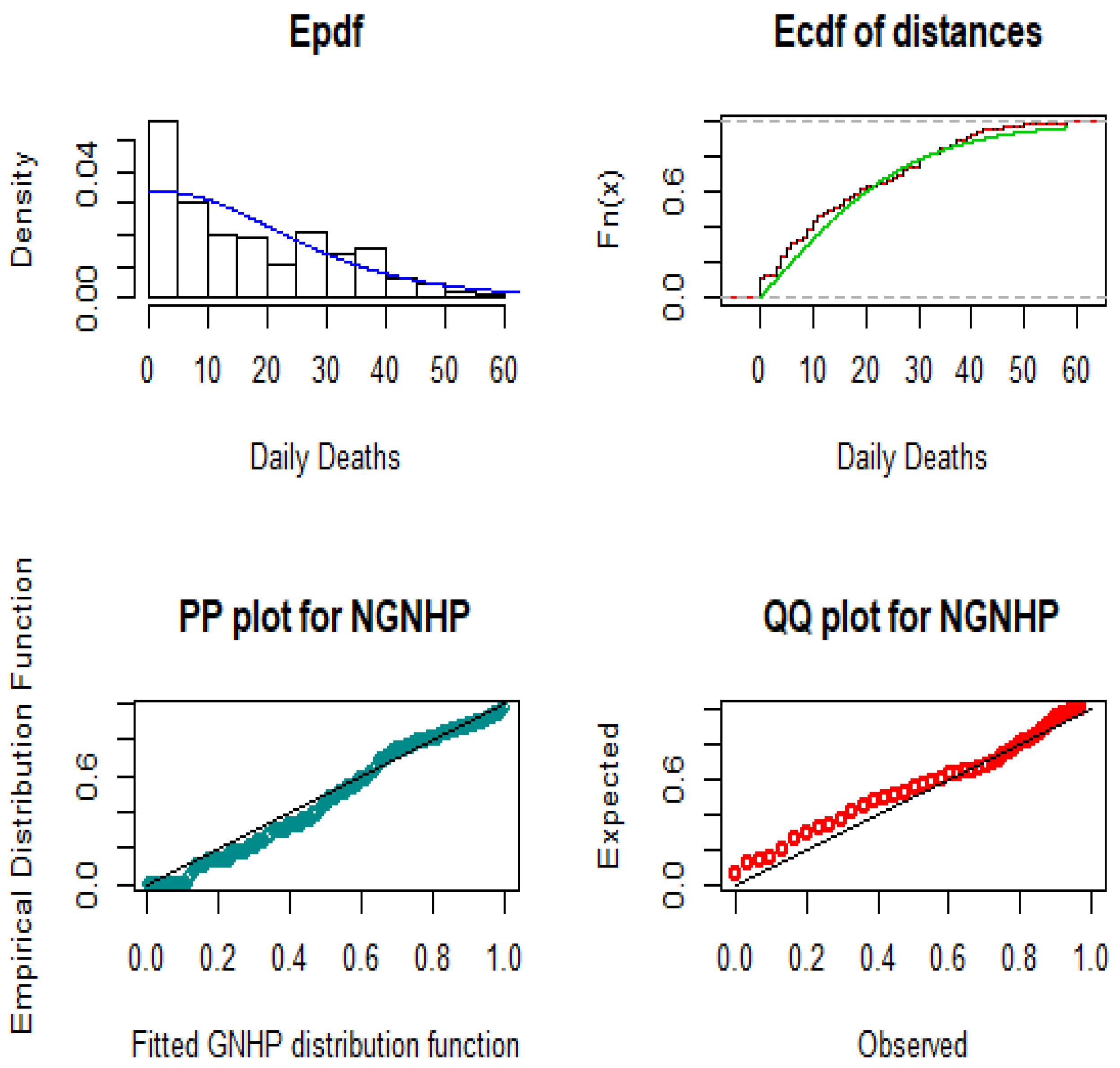
The fitted pdf, the fitted cdf, the probability–probability (PP) plot, and the quantile–quantile (QQ) plot of the NGNHP model for COVID-19 daily cases data in Egypt are presented in Figure 6. The fitted pdf, the fitted cdf, the PP plot, and the QQ plot of the NGNHP model for COVID-19 daily cases data in Saudi Arabia are also presented in Figure 7. Further, the fitted pdf, the fitted cdf, the PP plot, and the QQ plot of the NGNHP model for COVID-19 daily deaths data in Egypt are presented in Figure 8. Additionally, the fitted pdf, the fitted cdf, the PP plot, and the QQ plot of the NGNHP model for COVID-19 daily deaths data in Saudi Arabia are presented in Figure 9. The black lines of Ecdf and Epdf in Figure 6, Figure 7, Figure 8 and Figure 9 show the real behaviors of COVID-19 daily cases and daily deaths data in Egypt and Saudi Arabia, whereas the blue and green lines show the proposed NGNHP model’s performance.
To show how closely the proposed model fits COVID-19 daily cases and daily deaths data in Egypt and Saudi Arabia, the PP plots and QQ plots of the NGNHP model are provided in Figure 6, Figure 7, Figure 8 and Figure 9. From Figure 5, Figure 6, Figure 7 and Figure 8, we can see that the proposed model provides a close fit to COVID-19 daily cases and daily deaths data in Egypt and Saudi Arabia.
Figure 6, Figure 7, Figure 8 and Figure 9 illustrate that the proposed NGNHP model fits COVID-19 daily cases and daily deaths data in Egypt and Saudi Arabia very closely, leading to the conclusion that the proposed model performs well.
We presented a new class of statistical distributions in this paper that can model the incidents resulting from COVID-19 pandemic dynamics. We offered a forum for researchers to use our model recommendation and we anticipate that current researchers will use our model for this and other similar purposes.
7. Concluding Remarks
The situation with the global coronavirus pandemic is very threatening. However, it is the concern of governments and other responsible entities to provide correct statistics and figures to take any practicable necessary step, such as allocation of the requisite quarantine operations, calculation of the needed number of places in hospitals, determination of the extent of personal security, and determining the degree of isolation of infectious people, among others. Therefore, the proposed method of epidemic dynamics comparison can be used to evaluate the actual situation. Forecasts are potentially unpredictable, but it is important to estimate and convey this ambiguity in forecasting so that users can make the best choices possible. Forecast uncertainty can be measured by issuing probability predictions regarding possible observed events based on existing projections and historical findings and forecasts. Complete probability density functions or cumulative distribution functions may be used to generate such probabilistic forecasts. Probability predictions must be recalibrated on measurements as an inherent part of the forecasting phase since projections estimate the potential condition of model variables rather than current real-world measurable variables. Forecasters should issue estimates of the conditional probability distribution of the future observed quantity given the available sample of ensemble predictions. Furthermore, we introduced a new family of statistical models to provide the best description of COVID-19 events. We applied the proposed method to COVID-19 daily cases data and COVID-19 daily deaths data of Egypt and Saudi Arabia, and observed that the proposed model fitted the COVID-19 daily cases data and the COVID-19 daily deaths data very closely.
Author Contributions
Conceptualization, M.M.M. and E.M.A.E. methodology, M.M.M., S.M.M. and E.M.A.E.; software, M.M.M., M.A.F. and S.M.M.; formal analysis, M.M.M., M.A.F. and E.M.A.E.; writing—original draft preparation, M.M.M. and E.M.A.E.; writing-review and editing, M.M.M., M.A.F. and S.M.M.; project administration, M.M.M.; funding acquisition, M.A.F. All authors have read and agreed to the published version of the manuscript.
Funding
This research received no external funding.
Data Availability Statement
The data presented in this study are openly available in https://data.humdata.org/dataset/novel-coronavirus-2019-ncov-cases.
Conflicts of Interest
The authors declare no conflict of interest.
References
- Nesteruk, I. Comparison of the coronavirus pandemic dynamics in Europe, USA and South Korea. medRxiv 2020. [Google Scholar] [CrossRef]
- Nesteruk, I. Comparison of the coronavirus epidemic dynamics in Italy and mainland China. In Investigation of Dynamics of Coronavirus Spreading; ResearchGate: Berlin, Germany, 2020. [Google Scholar] [CrossRef]
- Nesteruk, I. Comparison of the coronavirus pandemic dynamics in Ukraine and neighboring countries. In Investigation of Dynamics of Coronavirus Spreading; ResearchGate: Berlin, Germany, 2020. [Google Scholar] [CrossRef]
- Zhao, J.; Ahmad, Z.; Almaspoor, Z.; El-Morshedy, M.; Afify, A.Z. Modeling COVID-9 Pandemic Dynamics in Two Asian Countries. Comput. Mater. Contin. 2021, 67, 965–977. [Google Scholar] [CrossRef]
- Zheng, Q.; Wang, X.; Bao, C.; Ma, Z.; Pan, Q. Mathematical modelling and projecting the second wave of COVID-19 pandemic in Europe. J. Epidemiol. Commun. Health 2021. [Google Scholar] [CrossRef]
- Giordano, G.; Blanchini, F.; Bruno, R.; Colaneri, P.; Di Filippo, A.; Di Matteo, A.; Colaneri, M. Modelling the COVID-19 epidemic and implementation of population-wide interventions in Italy. Nat. Med. 2020, 26, 855–860. [Google Scholar] [CrossRef]
- Anastassopoulou, C.; Russo, L.; Tsakris, A.; Siettos, C. Data-based analysis, modelling and forecasting of the COVID-19 outbreak. PLoS ONE 2020, 15, e0230405. [Google Scholar] [CrossRef] [Green Version]
- Naik, P.A.; Yavuz, M.; Qureshi, S.; Zu, J.; Townley, S. Modeling and analysis of COVID-19 epidemics with treatment in fractional derivatives using real data from Pakistan. Eur. Phys. J. Plus 2020, 135, 1–42. [Google Scholar] [CrossRef] [PubMed]
- Musa, S.S.; Qureshi, S.; Zhao, S.; Yusuf, A.; Mustapha, U.T.; He, D. Mathematical modeling of COVID-19 epidemic with effect of awareness programs. Infect. Dis. Model. 2021, 6, 448–460. [Google Scholar] [CrossRef] [PubMed]
- Alghamdi, M.; AlQarni, M.S.; Alshomrani, A.S.; Ullah, M.Z.; Baleanu, D. Dynamics of COVID-19 via singular and non-singular fractional operators under real statistical observations. Math. Methods Appl. Sci. 2020. [Google Scholar] [CrossRef]
- Langemann, D.; Nesteruk, I.; Prestin, J. Comparison of mathematical models for the dynamics of the Chernivtsi children disease. Math. Comput. Simul. 2016, 123, 68–79. [Google Scholar] [CrossRef]
- La Gatta, V.; Moscato, V.; Postiglione, M.; Sperli, G. An Epidemiological Neural network exploiting Dynamic Graph Structured Data applied to the COVID-19 outbreak. IEEE Trans. Big Data 2021, 7, 45–55. [Google Scholar] [CrossRef]
- Nadler, P.; Arcucci, R.; Guo, Y. A Neural SIR Model for Global Forecasting. Mach. Learn. Res. 2020, 136, 254–266. [Google Scholar]
- Alzaatreh, A.; Lee, C.; Famoye, F. A new method for generating families of continuous distributions. Metron 2013, 71, 63–79. [Google Scholar] [CrossRef] [Green Version]
- Al-Babtain, A.A.; Shakhatreh, M.K.; Nassar, M.; Afify, A.Z. A New Modified Kies Family: Properties, Estimation Under Complete and Type-II Censored Samples, and Engineering Applications. Mathematics 2020, 8, 1345. [Google Scholar] [CrossRef]
- Jayakumar, K.; Mathew, T. On a generalization to Marshall–Olkin scheme and its application to Burr type XII distribution. Stat. Pap. 2008, 49, 421–439. [Google Scholar] [CrossRef]
- Cordeiro, G.M.; Alizadeh, M.; Silva, R.B.; Ramires, T.G. A New Wider Family of Continuous Models: The Extended Cordeiro and de Castro Family. Hacet. J. Math. Stat. 2016, 47, 25. [Google Scholar] [CrossRef]
- Oluyede, B.O.; Warahena-Liyanage, G.; Pararai, M. A new compound class of log-logistic Weibull–Poisson distribution: Model, properties and applications. J. Stat. Comput. Simul. 2015, 86, 1363–1391. [Google Scholar] [CrossRef]
- Mansour, M.M.; Mohamed, S.M. A new generalized of transmuted Lindley distribution. Appl. Math. Sci. 2015, 9, 2729–2748. [Google Scholar] [CrossRef]
- Maurya, S.K.; Kaushik, A.; Singh, R.K.; Singh, S.K.; Singh, U. A new method of proposing distribution and its application to real data. Imp. J. Interdiscip. Res. 2016, 2, 1331–1338. [Google Scholar]
- Abouammoh, A.; Kayid, M. A New Family of Extended Lindley Models: Properties, Estimation and Applications. Mathematics 2020, 8, 2146. [Google Scholar] [CrossRef]
- Chen, Z. A new two-parameter lifetime distribution with bathtub shape or increasing failure rate function. Stat. Probab. Lett. 2000, 49, 155–161. [Google Scholar] [CrossRef]
- Mansour, M.M.; Ibrahim, M.; Aidi, K.; Butt, N.S.; Ali, M.M.; Yousof, H.M.; Hamed, M.S. A New Log-Logistic Lifetime Model with Mathematical Properties, Copula, Modified Goodness-of-Fit test for Validation and Real Data Modeling. Mathematics 2020, 8, 1508. [Google Scholar] [CrossRef]
- Tahir, M.H.; Hussain, M.A.; Cordeiro, G.M. A new flexible generalized family for constructing many families of distributions. J. Appl. Stat. 2021, 1–21. [Google Scholar] [CrossRef]
- Maurya, S.K.; Nadarajah, S. Poisson Generated Family of Distributions: A Review. Sankhya B 2020, 1–57. [Google Scholar] [CrossRef]
- Nadarajah, S.; Cancho, V.G.; Ortega, E.M.M. The geometric exponential Poisson distribution. J. Ital. Stat. Soc. 2013, 22, 355–380. [Google Scholar] [CrossRef]
- Nadarajah, S.; Haghighi, F. An extension of the exponential distribution. Statistics 2011, 45, 543–558. [Google Scholar] [CrossRef]
Figure 1.
Plots for COVID-19 daily cases and daily deaths in Egypt and Saudi Arabia.

Figure 2.
Plots for COVID-19 total number of cases (TC), total deaths (TD), total recovered (TR), and total active cases (TAC) in Egypt and Saudi Arabia.
Figure 2.
Plots for COVID-19 total number of cases (TC), total deaths (TD), total recovered (TR), and total active cases (TAC) in Egypt and Saudi Arabia.

Figure 3.
Histogram for COVID-19 daily cases, daily deaths, and daily recovered in Egypt and Saudi Arabia.
Figure 3.
Histogram for COVID-19 daily cases, daily deaths, and daily recovered in Egypt and Saudi Arabia.

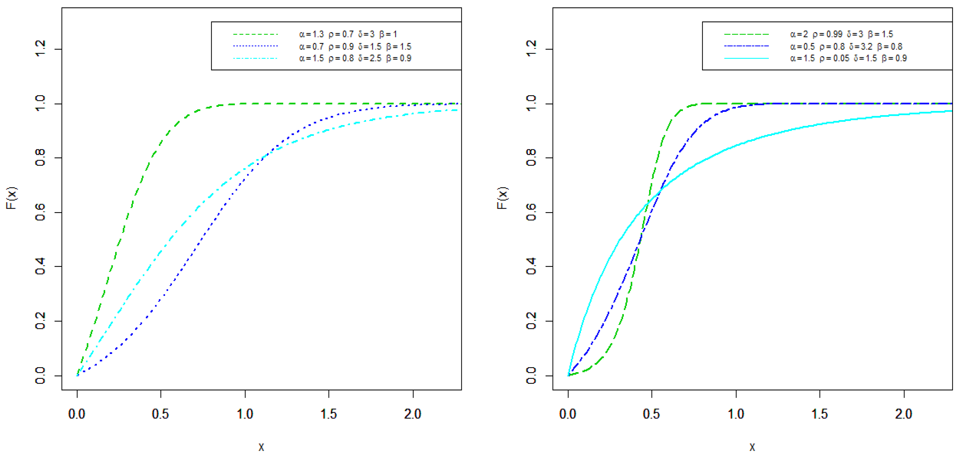
Figure 4.
Plots for the density function of the Nadarajah-Haghighi Poisson (NGNHP) distribution.

Figure 5.
Plots for the cdf of the NGNHP distribution.

Figure 6.
Estimated pdf, estimated cdf, probability–probability (PP) Plot, and quantile–quantile (QQ) plot of the NGNHP model for Egyptian COVID-19 daily cases data.
Figure 6.
Estimated pdf, estimated cdf, probability–probability (PP) Plot, and quantile–quantile (QQ) plot of the NGNHP model for Egyptian COVID-19 daily cases data.

Figure 7.
Estimated pdf, estimated cdf, PP Plot, and QQ plot of the NGNHP model for Saudi COVID-19 daily cases data.
Figure 7.
Estimated pdf, estimated cdf, PP Plot, and QQ plot of the NGNHP model for Saudi COVID-19 daily cases data.

Figure 8.
Estimated pdf, estimated cdf, PP Plot, and QQ plot of the NGNHP model for Egyptian COVID-19 daily deaths data.
Figure 8.
Estimated pdf, estimated cdf, PP Plot, and QQ plot of the NGNHP model for Egyptian COVID-19 daily deaths data.

Figure 9.
Estimated pdf, estimated cdf, PP Plot, and QQ plot of the NGNHP model for Saudi COVID-19 daily deaths data.
Figure 9.
Estimated pdf, estimated cdf, PP Plot, and QQ plot of the NGNHP model for Saudi COVID-19 daily deaths data.


Table 1.
Estimates of the model parameters for the data.
| Estimates of the MLEs of the Parameters | ||||
|---|---|---|---|---|
| Data | ||||
| Egyptian COVID-19’s daily cases data | 0.1461 | 0.9990 | 7632 | 0.1413 |
| Saudi COVID-19’s daily cases data | 0.0509 | 0.9985 | 7286 | 0.1327 |
| Egyptian COVID-19’s daily deaths data | 2.3845 | 0.6525 | 0.0106 | 2.2230 |
| Saudi COVID-19’s daily deaths data | 0.1576 | 0.5715 | 0.0715 | 1.009 |
Table 2.
Discrimination measures of the models for the data.
| AIC | CAIC | BIC | |
|---|---|---|---|
| Egyptian COVID-19’s daily cases data | 5094.923 | 5095.011 | 5110.566 |
| Saudi COVID-19’s daily cases data | 5560.234 | 5560.322 | 5575.877 |
| Egyptian COVID-19’s daily deaths data | 2976.485 | 2976.573 | 2992.129 |
| Saudi COVID-19’s daily deaths data | 2840.788 | 2840.876 | 2856.431 |
Publisher’s Note: MDPI stays neutral with regard to jurisdictional claims in published maps and institutional affiliations. |
© 2021 by the authors. Licensee MDPI, Basel, Switzerland. This article is an open access article distributed under the terms and conditions of the Creative Commons Attribution (CC BY) license (https://creativecommons.org/licenses/by/4.0/).
Share and Cite
MDPI and ACS Style
Mansour, M.M.; A. Farsi, M.; Mohamed, S.M.; Abd Elrazik, E.M. Modeling the COVID-19 Pandemic Dynamics in Egypt and Saudi Arabia. Mathematics 2021, 9, 827. https://doi.org/10.3390/math9080827
AMA Style
Mansour MM, A. Farsi M, Mohamed SM, Abd Elrazik EM. Modeling the COVID-19 Pandemic Dynamics in Egypt and Saudi Arabia. Mathematics. 2021; 9(8):827. https://doi.org/10.3390/math9080827
Chicago/Turabian StyleMansour, Mahmoud M., Mohammed A. Farsi, Salah M. Mohamed, and Enayat M. Abd Elrazik. 2021. "Modeling the COVID-19 Pandemic Dynamics in Egypt and Saudi Arabia" Mathematics 9, no. 8: 827. https://doi.org/10.3390/math9080827
Note that from the first issue of 2016, this journal uses article numbers instead of page numbers. See further details here.