

Abstract
The COVID-19 pandemic and ensuing lockdown of many US States resulted in rapid changes to motor vehicle traffic and their associated emissions. This presents a challenge for air quality modelling and forecasting during this period, in that transportation emission inventories need to be updated in near real-time. Here, we update the previously developed fuel-based inventory of vehicle emissions (FIVE) to account for changes due to COVID-19 lockdowns. We first construct a 2020 business-as-usual (BAU) case inventory and adjust the emissions for a COVID-19 case using monthly fuel sales information. We evaluate cellular phone-based mobility data products (Google COVID-19 Community Mobility, Apple COVID-19 Mobility Trends) in comparison to embedded traffic monitoring sites in four US cities. We find that mobility datasets tend to overestimate traffic reductions in April 2020 (i.e. lockdown period), while fuel sales adjustments are more similar to changes observed by traffic monitors; for example, mobility-based methods for scaling emissions result in an approximately two-times greater estimate of on-road nitrogen oxide (NOx) reductions in April 2020 than we find using a fuel-based method. Overall, FIVE estimates a 20%–25% reduction in mobile source NOx emissions in April 2020 versus BAU, and a smaller 6%–7% drop by July. Reductions in April showed considerable spatial heterogeneity, ranging from 6% to 39% at the state level. Similar decreases are found for carbon monoxide (CO) and volatile organic compounds. Decreases to mobile source NOx emissions are expected to lower total US anthropogenic emissions by 9%–12% and 3%–4% in April and July, respectively, with larger relative impacts in urban areas. Changes to diurnal and day-of-week patterns of light- and heavy-duty vehicular traffic are evaluated and found to be relatively minor. Beyond the applicability to modelling air quality in 2020, this work also represents a methodology for quickly updating US transportation inventories and for calibrating mobility-based estimates of emissions.
Export citation and abstract BibTeX RIS

Original content from this work may be used under the terms of the Creative Commons Attribution 4.0 license. Any further distribution of this work must maintain attribution to the author(s) and the title of the work, journal citation and DOI.
1. Introduction
Beginning in January of 2020, the international spread of the COVID-19 virus incurred policy interventions on mobility (e.g. 'lockdowns') by governments throughout the world, causing unprecedented decreases to vehicle traffic (Parr et al 2020, FHWA 2020c). Studies have indicated that these changes in traffic directly affected air pollution, as presently reported in China (Chen et al 2021) and the United States (Xiang et al 2020). Ground monitoring data in numerous US cities indicate that statistically significant reductions to nitrogen dioxide (NO2) concentrations occurred in April relative to previous years (25.5%, Berman and Ebisu 2020; 19%–49%, Chen et al 2020). Changes of similar magnitude have also been observed in Europe (Barré et al 2021) and China (Wang et al 2020). Satellite-based retrievals of NO2 column concentrations have also been used to observe declines across the US (19%–28%, Bauwens et al 2020; 30%, Blumberg 2020; 21.6%, Goldberg et al 2020) and Europe (Barré et al 2021). The response of secondary air pollutants such as fine particulate matter (PM2.5) and ozone has been smaller or even opposite that of the decreases in NO2 owing to atmospheric chemistry (Berman and Ebisu 2020, Chen et al 2020, Wang et al 2020).
The global COVID-19 lockdowns present a unique opportunity for assessing how different emission sectors, particularly the mobile source sector, impact air quality. Previous studies (Tong et al 2015) have highlighted a need for timely updates to emission inventories used in air quality models and forecasting, which may otherwise take years to develop. Although many studies have investigated the effects that the lockdown has had on air pollution, fewer have attempted to estimate bottom-up emissions for this period (Guevara et al 2021, Huang et al 2021). Global inventories have updated mobile source emissions using COVID-19 mobility datasets (Doumbia et al 2021, Forster et al 2020, Le Quere et al 2020, Liu et al 2020, Pompomi et al 2021), such as those published by Google and Apple, which evaluate changes in human mobility with data derived from mobile phone locations and queries. Using mobility datasets, Forster et al (2020) and Doumbia et al (2021) estimate that total US nitrogen oxides (NOx ) emissions decreased by 40% and 21%, respectively, in April. Also using mobility datasets, Le Quere et al (2020) and Liu et al (2020) estimate that monthly US surface transportation carbon dioxide (CO2) emissions fell by 42% and 50% respectively, at a maximum. In comparison to estimates based on ground or satellite measurements (Goldberg et al 2020, Keller et al 2020), some mobility-based estimates of NO2 reductions are notably greater.
The mobile source sector is composed of both on-road and off-road engines. When considering US on-road sources, gasoline is consumed primarily by light-duty (LD) vehicles and diesel by heavy-duty (HD) trucks. In the previous decades, mobile source NOx emissions have been decreasing even while the relative contribution of on-road diesel grew, due to successes (e.g. three-way catalysts) in controlling on-road gasoline emissions (Dallmann and Harley 2010, McDonald et al 2012). Within the US, mobile sources make up 53% of anthropogenic NOx emissions (EPA 2017) and are disproportionately located in cities (McDonald et al 2014), hence their importance for assessing urban air quality impacts of the COVID-19 pandemic. The US in particular experienced a patchwork of different state and local public health responses to the pandemic, suggesting non-uniform trends in traffic (Chen et al 2020, Raifman et al 2020). Previous studies have found that HD traffic has a disproportionate contribution to transportation NOx and PM2.5 emissions, relative to LD traffic (Dallmann and Harley 2010, McDonald et al 2012, 2015), which can lead to inequities in primary air pollutant exposure among lower income and non-white populations (Demetillo et al 2020). Lockdown effects may also play out differently for LD and HD traffic (Archer et al 2020, Dantas et al 2020) due to varying impacts of the pandemic on personal and commercial movement, indicating the importance of capturing these trends independently. Additionally, it has been observed that urban and densely populated areas in the US have experienced greater changes to both traffic (Parr et al 2020) and air pollution (Berman and Ebisu 2020, Chen et al 2020) than rural areas due to COVID-19 lockdowns.
Here, we first develop a 2020 business-as-usual (BAU) inventory, following the fuel-based methodology of McDonald et al (2014). In assessing a means for estimating mobile source emissions COVID-19 scaling factors, we investigate using COVID-19 mobility datasets from Apple (Apple 2020) and Google (Google 2020) against using fuel sales trends. In doing so, we aim to quantify changes in US gasoline and diesel consumption throughout the COVID-19 pandemic, using monthly fuel sales data, which have previously been utilized to develop regional and national-scale mobile source emission inventories (Kim et al 2016, McDonald et al 2018a). We also aim to determine whether COVID-19 lockdowns have affected diurnal and day-of-week traffic patterns. Finally, this information can be used to quantify changes in mobile source emissions of CO2 and co-emitted air pollutants, including carbon monoxide (CO), NOx , volatile organic compounds (VOCs), ammonia (NH3), sulphur dioxide (SO2), and PM2.5. The result is a gridded 2020 monthly mobile source emissions inventory, for the contiguous US, with BAU and COVID-19 perturbed emissions cases, which can be utilized in air quality models.
2. Methods
2.1. Mapping BAU on-road fuel consumption
We follow the methodology developed by McDonald et al (2014) to update the spatial mapping of the fuel-based inventory for vehicle emissions (FIVE). The most recent national traffic count data are available at a roadway-link level from the highway performance monitoring system (HPMS) for the year 2018 (FHWA 2020a), which spatially allocate ∼82% and ∼71% of LD and HD traffic, respectively, when compared with state-level traffic statistics (FHWA 2020b). In the US, gasoline is consumed primarily by LD vehicles and diesel by HD vehicles. Therefore, we use LD traffic data to downscale annual state-level taxable gasoline sales (FHWA 2020b), and HD traffic for diesel sales. Untaxed diesel consumption by buses is also included (Davis and Boundy 2020). The 2018 fuel use maps are then projected to 2019 (BAU fuel is assumed unchanged from 2019 to 2020) using the state-level taxable fuel sales records of gasoline and diesel. For simplicity, the balance of traffic unaccounted by HPMS traffic count data is spatially apportioned using population as a surrogate (EPA 2020). While distributing on-road emissions by population density is known to introduce bias (Gately et al 2015), this is diminished by the large portion of fuel consumption already distributed at the roadway link level. The result is a gridded 4 km × 4 km contiguous US emissions map of on-road fuel consumption, separately apportioned between LD and HD traffic.
2.2. Mapping off-road mobile source engine activity
Off-road gasoline engines consist of small two- and four-stroke gasoline engines (e.g. lawn equipment, generators, forklifts, recreational vehicles, watercraft), consuming ∼6% of total gasoline (FHWA 2020b). Though this consumption is relatively small, it can be a significant source of CO and VOCs due to high emission factors relative to on-road transportation (Gordon et al 2013). Off-road diesel engines are used in heavy equipment (e.g. agricultural, construction, other industrial/commercial engines), and are important sources of NOx and PM (Dallmann and Harley 2010). Off-road diesel fuel use is estimated following Kean et al (2000), utilizing end-use surveys reported by the Energy Information Administration (EIA) (EIA 2019). Off-road fuel use is mapped utilizing spatial and temporal surrogates from the National Emissions Inventory (NEI) 2011 (EPA 2014) for two- and four-stroke gasoline equipment, small watercraft, and agricultural and non-agricultural diesel engines (McDonald et al 2018a). While there are more recent versions of the NEI, spatial and temporal surrogates are not expected to change significantly until the US 2020 Census is complete.
2.3. Accounting for changes in mobile source activity due to COVID-19
2.3.1. Monthly scaling factors of gasoline and diesel fuel sales
To estimate scaling factors between BAU (assumed unchanged from 2019) and the COVID perturbed case, we use the EIA's prime supplier sales volumes (PSSV) (EIA 2020), which report sales of gasoline and diesel fuel into regional markets, allowing separate LD and HD trends to be quantified. We develop BAU to 2020 COVID case monthly fuel scaling factors first at a Petroleum Administration for Defence District (PADD) level, which cover five regions of the US (East Coast, Midwest, Gulf Coast, Mountain West, and West Coast). For on-road sources, PADD-level fuel scalings are then downscaled to the state level using monthly state traffic volumes (FHWA 2020c). Scaling factor calculations are described in appendix S1 (available online at stacks.iop.org/ERL/16/065018/mmedia), and tables S1 and S2. PSSV does not distinguish between fuel consumed by on-road and off-road engines, and hence we use PADD-level fuel sales as the basis for both on-road and off-road fuel scaling factors. We later test this assumption by assessing ambient monitoring data of NOx /CO.
2.3.2. Traffic monitoring data
Traffic monitoring data are used to evaluate COVID-19 mobility datasets and assess whether traffic speed or typical diurnal and day-of-week traffic patterns (McDonald et al 2014) have been altered due to COVID-19. Table S3 lists sources of real-time and publicly available traffic monitoring data from four locations: (a) Los Angeles, (b) San Francisco, (c) Atlanta, and (d) New York City. These four cities represent large population centres across the country. Nationally, interstate highway traffic is reported weekly by the FHWA, based on embedded traffic counters (FHWA 2020d). A map of urban monitoring locations (figure S1) and further details (appendix S2) are included.
2.4. Mobile source emission factors
Based on previous studies described below, we compile fuel-based mobile source emission factors (in g kg−1 fuel) for CO, NOx , VOCs, NH3, SO2, and PM2.5 for the 2020 BAU year (table S4). A brief description of the methodology is provided here, and more detail can be found in appendix S3, appendix S4 and table S5.
On-road fuel-based emission factors used in FIVE for CO, NOx , and VOCs have been described by several studies (McDonald et al 2012, 2013, 2018a, 2018b, Hassler et al 2016). Emission factors are adjusted to account for the effects of cold-starting engines based on the EPA MOVES2014a model (EPA 2015), as well as evaporative emissions of gasoline (see appendix S4 and table S5 for details). Primary PM2.5 emission factors from gasoline and diesel exhaust have been described by McDonald et al (2015). Trends in LD PM2.5 exhaust emissions scale with CO (McDonald et al 2015), and we update HD PM2.5 exhaust emission factors with more recent measurements of HD trucks (figure S2). We also include brake wear and tire wear emissions from the EPA MOVES2014a model (EPA 2015). Cao et al (2021) presents trends in tailpipe NH3 emission factors. Lastly, the SO2 emission factor is estimated based on a sulphur content of 10 ppm and 20 ppm (by weight) for gasoline and diesel fuel, respectively.
For off-road engines, we use emission factors from the EPA NONROAD model (EPA 2010), except where otherwise noted in table S4 for off-road gasoline engines. Off-road gasoline CO, NOx , VOC, and PM2.5 emission factors have been described previously for FIVE (McDonald et al 2015, 2018a, 2018b). Emission factors of SO2 are assumed to be the same for on-road gasoline and diesel engines. Since 2014, all non-road engines are required to utilize ultra-low sulphur diesel (EPA 2017).
3. Results and discussion
3.1. Analysis of COVID-19 mobility datasets
In figure 1, we compare Apple's COVID-19 Mobility Trends Report (Apple 2020) and Google's COVID-19 Community Mobility Report (Google 2020) with highway traffic monitoring data across four cities (figure 1: (a) New York, (b) San Francisco, (c) Atlanta and (d) Los Angeles). For Google's mobility report, we average the Workplace Mobility and the Retail and Recreation Mobility metrics. For Apple's mobility report, we use the driving mobility index. We note that neither mobility report attempts to directly quantify changes to on-road transportation. Google's report is derived from mobile phone location activity at marked locations while Apple's report is derived from Apple Maps personal vehicle routing requests. Additionally, the Apple and Google mobility datasets do not explicitly capture HD traffic trends, which are important to on-road trends due to differences in emission factors by engine type (table S4).
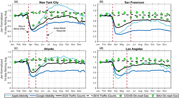
Figure 1. Comparison of COVID-19 Mobility Datasets (Apple and Google) relative to 2020 traffic monitoring data for (a) New York City, (b) San Francisco, (c) Atlanta, and (d) Los Angeles. Each trend line is normalized to their January values and shown as a 14 days rolling average. Blue lines are 2020 mobility dataset trends: (light blue) Apple's driving mobility dataset and (dark blue) the average of Google's Workplace and Retail/Recreation Mobility datasets. Black lines are 2019 (dashed) and 2020 (solid) traffic trends, compiled from embedded roadway counters in each city (table S3). Green markers are BAU and COVID case on-road gasoline scaling factors (described in section 3.2). Vertical dashed red lines illustrate lockdown (stay-at-home orders) and reopening (indoor retail allowed) dates (see table S6).
Download figure:
Standard image High-resolution imageConsidering the mobility datasets alone, we find they perform similarly in capturing the beginning of lockdowns (figure 1). When comparing timing of decreases in traffic monitoring and mobility to timing of public health measures, traffic decreases generally precede stay-at-home orders (table S6) by several weeks. Apart from Atlanta, reopening measures do not generally coincide with a significant traffic increase. Traffic counters in each city (black lines in figure 1) show that by July, traffic has nearly recovered from the minimum in travel seen in April. In June and beyond, Google's datasets have not recovered to prior levels, whereas Apple's dataset shows a stronger recovery, and even exceeds 2019 traffic levels in some cities.
Across the cities considered, neither mobility dataset performs well at capturing trends in 2020 traffic. Considering the month of April, normalized mean bias relative to traffic counters of Google mobility data is −29% and −27% for Apple (figure 1). Considering the COVID-19 timeframe from March to December, biases are −28% for Google (R = 0.72) and +5% for Apple (R = 0.80). While Apple mobility data exhibits little overall bias, the direction and magnitude of bias varies largely by month and location (figure 1). For Google, the bias is more consistent throughout the year but varies by location.
While the mobility datasets evaluated here may not precisely capture the magnitudes of traffic trends, their value for rapidly understanding the onset of the pandemic and general traffic trends should not be underestimated. Mobility datasets are daily estimates, available within a few days at a county-level spatial resolution. With proper calibration of the relationship between mobility data and traditional traffic counting and fuel sales data used in bottom-up emission inventories (Gurney et al 2012, Gately et al 2013, McDonald et al 2014), these datasets could be improved for future research and air quality forecasting efforts. As an alternative to using mobility data to estimate COVID-19 emission scaling factors, and to facilitate future use of mobility datasets, we next explore scalings based on monthly fuel sales data.
3.2. Impacts of COVID-19 on gasoline and diesel fuel sales
Figure 2 shows changes in US gasoline (panel a) and diesel (panel b) fuel sales, as well as a map of 2020 BAU on-road CO2 emissions with reductions due to COVID-19 lockdowns by PADD district overlaid (panel c). Fuel sales data are de-seasonalized by representing each month as a fraction relative to the same month in 2019. Under BAU conditions, on-road traffic peaks in summer and is lower in winter (McDonald et al 2014), so a de-seasonalized trend better portrays how COVID-19 lockdowns impact transportation. The coloured uncertainty bands reflect regional variability at a PADD level. Although fuel sales trends are similar across PADDs (figures 2(a) and (b)), variations in the fraction of total on-road fuel consumed as diesel result in on-road CO2 reductions (figure 2(c)) that are 35% larger in the most affected PADD than the least affected PADD (PADD scaling factors included in table S7). The PADD district to state-level downscaling we apply to on-road LD activity (appendix S1) suggests even greater variability in fuel sales when examined by state rather than by region (green error bars shown in figure 2(a), table S8).
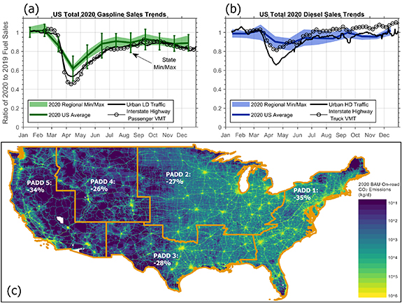
Figure 2. Ratio of 2020 versus 2019 (a) gasoline and (b) diesel fuel sales by month. The coloured band represents regional variability at the PADD-level (orange boundaries in panel c). Green error bars in gasoline sales represent variability across states. Also shown are urban traffic monitoring data (solid black line) averaged across New York City, Atlanta, Los Angeles, and San Francisco and the sum of interstate traffic nationally (open circle black line). (c) Reduction in on-road CO2 emissions in April 2020 versus business-as-usual at 4 km × 4 km resolution and summarized by PADD region.
Download figure:
Standard image High-resolution imageOverall, we estimate US states experienced 25%–51% decreases in gasoline sales in April 2020, relative to April 2019. Traffic and fuel sales both decrease in March and reach a minimum in April as lockdown measures go into effect (figure 2(a)). Public health policies surrounding the reopening of states have been staggered and vary by state, but in both traffic and fuel sales we observe that most of the recovery occurs in May and June. Traffic recovery then plateaus and remains below normal throughout July and August. By July, we estimate gasoline sales decreased 1%–15% across states, relative to 2019 levels.
We also compare gasoline fuel sales trends with LD traffic trends from publicly available embedded traffic counters at urban and national scales. The urban locations included are the same as in figure 1. Generally, we observe that both urban only and national LD traffic on interstates follow a similar trend throughout 2020, which also follow the gasoline fuel sales trend line (figure 2(a)). In contrast, diesel sales follow a different monthly pattern throughout 2020 (figure 2(b)). In April 2020, diesel sales decreased by 4%–17% relative to 2019. Urban HD traffic has a greater decrease in April 2020 (−30%) than national interstate HD traffic (−16%) by a factor of ∼2, a difference not apparent in LD traffic. This suggests that intra-city HD truck traffic was impacted greater than interstate goods movement. We provide COVID-19 inventory scaling factors for LD/HD traffic separated by urban and rural regions in table S8 (see appendix S1 for methodology).
State-level on-road gasoline fuel scalings are plotted for the four cities in figure 1. The April fuel scalings we develop exhibit less normalized mean bias relative to monthly averaged traffic counting data (+12%) than monthly averaged mobility data (−29%, Google; −27%, Apple). Between March and December, bias in our fuel scalings is +8%, which outperforms Google mobility (−28%). Bias in Apple's dataset is smaller (+5%) due to offsetting directions in the bias throughout the year across locations. Over the same timeframe, our fuel scalings have lower normalized mean absolute error (NMAE = 0.09) compared to either mobility dataset (NMAE = 0.28, Google; NMAE = 0.17, Apple). Fuel scalings also correlate with traffic counters (R = 0.90) better than for mobility data (R = 0.72, Google; R = 0.80, Apple). While a state-level fuel-based method has reasonable bias and correlation with respect to traffic counters, a positive bias in each city suggests our fuel-based scaling may slightly overestimate urban traffic throughout 2020. Further research is needed to separate urban and city-level variations in traffic from state-level variations, such as top-down emissions estimate techniques using high-spatial resolution satellite data (e.g. TROPOMI).
3.3. Evaluating changes in traffic speed, and diurnal and day-of-week traffic patterns
Traffic volume reductions in 2020 likely impacted speed patterns, which affect vehicle fuel consumption rates. We investigate this by looking at highway speeds in several locations. In Los Angeles, the average highway speed increased +17% (84 km h−1 to 98 km h−1) in April 2020 versus April 2019. Similar trends are found in San Francisco (+18%, 87 km h−1 to 103 km h−1) and Atlanta (+21%, 89 km h−1 to 108 km h−1). Throughout the rest of the 2020, highway speed increases averaged +10%, +16% and +9% for Los Angeles, San Francisco, and Atlanta, respectively. While a reduction in stop-and-go congestion improves fuel economy, high speed driving exceeding 90 km h−1 also degrades fuel economy and could offset fuel economy gains from reduced congestion (Davis and Boundy 2021). While spatially resolved speed information could help improve our bottom-up emissions inventory at finer spatial scales, at coarser resolutions (e.g. state-level), fuel sales data reflect the combined effect of changes in the amount of driving and in fuel economy. For co-emitted air pollutants, fuel-based emission factors are much less sensitive to changes in speed and engine loading in comparison to activity-based emission factors (i.e. g km−1) (Bishop and Stedman 2008, McDonald et al 2013, McDonald et al 2018a). This implies that reductions in fuel use also translate to similar reductions in co-emitted air pollutants.
When examining changes to weekday passenger diurnal traffic patterns throughout 2020 versus 2017–19, we find insignificant changes during morning (5–9 AM) and evening (2–6 PM) rush hours, by +1% and +6%, respectively (figure S3). Daytime truck traffic (6 AM—6 PM) in April also changes insignificantly by +4% (figure S4). For LD and HD vehicles, weekday traffic saw minor increases while weekend traffic saw minor decreases (figure S5). In the months following April, the magnitude of these deviations decreases. Traffic monitoring data aggregated at a state level, typically has 95% confidence bounds of ±15%–19% (FHWA 2016), meaning that the changes in day-of-week and diurnal traffic patterns due to COVID-19 are likely not statistically significant relative to uncertainties in traffic monitoring datasets. In general, we find that while the overall level of traffic changed due to the COVID-19 pandemic, the timing of traffic was not significantly altered.
3.4. 2020 mobile source emissions
Figure 3 presents a map of COVID-19 changes to mobile source NOx emissions (panel a) and their impact on total anthropogenic NOx emissions (panel b) for the month of April. Non-mobile emissions (e.g. industry and power plants) are from the NEI 2017 (EPA 2020) and are not adjusted, thus our estimates of how total anthropogenic emissions have changed due to COVID-19 should be treated as a lower bound estimate as other emission sectors have likely been impacted by the pandemic. The fuel sales data used in estimating fuel scaling factors include both on-road and off-road mobile source engines, and we apply the same fuel scaling factors to both types of engines at a PADD level. Ambient NOx /CO ratios in 2019 and 2020 are assessed by month (see figure S6 and appendix S5), a diagnostic previously used to evaluate mobile source emission inventories (Parrish et al 2006, McDonald et al 2013, Hassler et al 2016). For Los Angeles and New York City, ambient NOx /CO stayed remarkably similar in 2019 and 2020, suggesting that the mix of gasoline and diesel fuel use has not changed in urban areas during the COVID-19 pandemic though overall activity levels are down.

Figure 3. (a) Percent change in April 2020 versus business-as-usual mobile source NOx emissions only by state. (b) Percent change in April 2020 versus business-as-usual total NOx emissions resulting from mobile source reductions only. Other non-mobile source emissions are left unadjusted.
Download figure:
Standard image High-resolution imageAt a state level, reductions to April NOx emissions vary between 6% and 39% (figure 3(a)) for mobile source emissions, which are expected to lower total anthropogenic emissions by 1%–26% (figure 3(b)). Summed over the contiguous US during the month of April, mobile source NOx emissions decreased 20%–25% (figure S7(a)), which lowers total anthropogenic NOx emissions by 9%–12% (figure 4(c)). The recovery in emissions reductions is steady throughout May and June but slows in July and beyond, where emissions remain below normal (figure S8). In July, NOx reductions are limited to 6%–7% (mobile sources) and 3%–4% (total), respectively (figures S7(b) and 4(d)). Overall, we find that 2020 NOx reductions are greatest for East and West Coast states, where transportation appears to be more impacted by public health measures to combat the spread of COVID-19. Additionally, in many coastal states, diesel fuel makes up a smaller fraction of on-road fuel consumption than in central states. For example, in Wyoming 52% by volume of on-road fuel consumption is diesel whereas only 17% is diesel in California (FHWA 2020b). Diesel consumption was not as heavily impacted by COVID-19 lockdowns as gasoline (figure 2), which helps to explain the greater relative decrease in mobile source NOx emissions in California versus Wyoming.
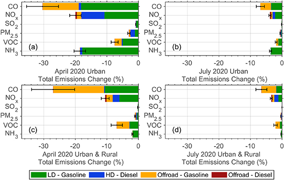
Figure 4. Percent change in US anthropogenic emissions in April 2020 versus business-as-usual summed across (a) urban and (b) urban and rural areas. Non-mobile source emission sectors (e.g. industry, power plants, etc) are not adjusted. Error bars represent uncertainty in fuel consumption and fuel emission factors (table S4) (right column). Same as (left column) except for July 2020.
Download figure:
Standard image High-resolution image
Lastly, we assess the impact COVID-19 lockdowns had on emissions in urban areas. In figure 4, we present a sectoral breakdown of mobile source related total emissions reductions in urban areas (figures 4(a) and (b)) and across the contiguous US (figures 4(c) and (d)) in April and July. Urban is defined by the US Census Bureau, as >1000 people mi−2 (386 people km−2). In both urban areas and across the contiguous US, COVID-19 related reductions to highly impacted pollutants such as CO, NOx , and NH3, are generally dominated by on-road and off-road gasoline, due to greater reductions in gasoline sales than diesel sales. The impacts on emissions we estimate are also relatively larger in urban areas than across the whole US (figure 4(c)) or in rural areas. We estimate that mobile source reductions lower total urban CO emissions by 25%–35% and total urban NOx emissions by 18%–22% in April (figure 4(a)), which are larger than the 20%–34% and 9–12%, respectively, reductions seen nationally (figure 4(c)). By July, total emissions reductions from mobile sources, as well as the enhanced reductions to urban emissions that we estimate, have greatly diminished (figures 4(b) and (d)).
Keller et al (2020) estimates a ∼30% decrease to NOx emissions in the US in April. The NO2 monitors used in their analysis are located predominantly in urban areas, meaning their estimate may better reflect urban reductions than total US reductions. Adjusting mobile sources alone (67% of urban NOx emissions), we estimate an 18%–22% decrease to urban NOx emissions, similar to Keller et al. If we accounted for COVID-19 impacts for other sources of NOx (e.g. industry), then it is possible that the inventory-observation agreement could be closer. Our urban reduction estimate (figures 4(a) and (b)) is also comparable to the decreases in tropospheric column NO2 observed by TROPOMI over US cities, when meteorology and seasonality are accounted for (Goldberg et al 2020). Specifically, we estimate reductions of 17%, 30%, and 35%, for New York City, Atlanta, and Los Angeles, respectively, compared to the mean decreases reported by Goldberg et al (2020) of 20%, 27%, and 33%.
Finally, our estimate of maximum change to on-road CO2 emissions (−31%, figure S7(c)) is notably less than estimates by Doumbia et al (2021), Forster et al (2020), and Liu et al (2020) (−40%, −45% and −50% respectively), which is likely due to using the fuel-based, rather than mobility-based, method presented here. While these studies do not separate LD and HD traffic trends, their on-road CO2 emission scalings can be applied to on-road NOx emissions, resulting in a mean mobility-based estimate of US on-road NOx reductions of 45% in April. These mobility-based reduction estimates are twice as large for US on-road NOx emissions in April compared to our fuel-based method (22%, figure S7(c)), which demonstrates both the importance of separating LD and HD trends and the need for calibrating the relationship between mobility datasets and traffic when scaling emissions.
4. Conclusions
In this work we present an analysis of COVID-19 mobility datasets against highway traffic monitoring. As an alternative to using COVID-19 mobility datasets, we demonstrate that a fuel-based method is also capable of updating US mobile source emissions on a near real-time basis, with results that better approximate traffic trends. An advantage of a fuel-based approach is the separate accounting of gasoline and diesel engines. The gridded FIVE emissions inventory is presented for January through December for a BAU and COVID-19 perturbed case of 2020 and made available online (Harkins et al 2021). The inventory files are monthly and those who use the data for chemical transport modelling should note the limitations of monthly estimates when modelling a period of rapidly changing emissions. This is particularly true for March 2020, where monthly estimates cannot capture the rapid drop in emissions.
We estimate that 2020 US mobile source NOx emissions were at a minimum in April, causing total anthropogenic emissions to decrease by 9%–12%. Based on fuel sales and traffic monitoring, US mobile source NOx emissions have recovered from April and are close to BAU emission levels by July (lowers total anthropogenic NOx emissions by 3%–4%). Additionally, while mobile source fuel consumption occurs primarily by on-road engines, off-road sources are important contributors to CO, NOx , and VOCs, and their emissions also need to be considered. Finally, this study suggests that mobility-based on-road emissions scaling factors may overestimate emissions reductions when compared to fuel-based methods. We suggest fuel-based methods as a means for calibrating the relationship between mobility and emissions, for use in areas where fuel consumption data are not broadly or rapidly available. While the focus of this study is on how mobile source emissions have changed in the US due to the COVID-19 pandemic, future work will include developing COVID-19 scaling factors for non-mobile source sectors, such as industry, power generation, and consumer products.
Acknowledgments
This study was supported by NOAA NRDD Project (#19533)—'COVID-19: Near Real-time Emissions Adjustment for Air Quality Forecasting and Long-Term Impact Analyses', the NOAA Cooperative Agreement (NA17OAR4320101), and NASA ROSES ACMAP (80NSSC19K0950). We thank Dr Gregory Frost (NOAA) for his support of this project and Dr Stuart McKeen (NOAA/CIRES) for his help in processing gridded emission files.
Data availability statement
The data that support the findings of this study are openly available at the following URL/DOI: https://csl.noaa.gov/groups/csl7/measurements/2020covid-aqs/emissions/.