
Modelling the Degree of Emotional Concern: COVID-19 Response in Social Media


1
Department of Computer Science and Artificial Intelligence, Universidad de Granada, 18010 Granada, Spain
2
E.ON SE, 45131 Essen, Germany
3
Mathematical Institute, University of Oxford, Oxford OX2 6GG, UK
*
Author to whom correspondence should be addressed.
Appl. Sci. 2021, 11(9), 3872; https://doi.org/10.3390/app11093872
Submission received: 16 March 2021
/
Revised: 19 April 2021
/
Accepted: 21 April 2021
/
Published: 25 April 2021
(This article belongs to the Special Issue Soft-Computing-Based Decision Support Systems on the Web)
Abstract
:The massive impact caused by the COVID-19 pandemic has left no one indifferent, becoming an unprecedented challenge. The use of protections such as sanitary masks has become increasingly common, restrictions in our daily lives, such as social distancing or confinements, have had serious consequences on the economy and our welfare state. Although the measures imposed throughout the world follow the same pattern, they have been applied with different criteria depending on the country. Over extended periods of time, people tend to change their perception of an event and its magnitude, or in other words, they stop being so concerned despite the seriousness of the matter. In this paper, we introduce a new metric to quantify the degree of emotional concern of people being affected by a topic, and we confirm how populations from different countries follow this trend of downplaying the effect of the pandemic and reach a state of indifference. To do this, we propose a method to analyze the social media stream over time extracting the different emotional states from the Russel Circumplex plane and computing the shifting created by the tragic event—the pandemic. We complete this metric by incorporating searching behavior to reflect not only push contents but also pull inquiries. The resulting metric establishes a relationship between the pandemic and the emotional response by defining the degree of Emotional Concern. Although the method can be applied to any location with a significant and varied amount of geo-localized social media streams, the scope of this paper covers the most representative cities in Europe.
1. Introduction
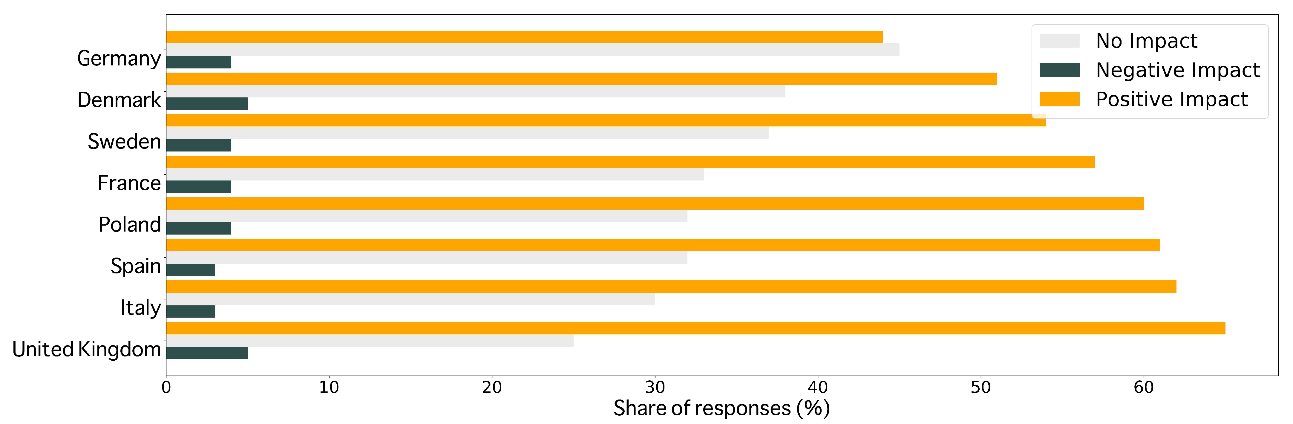
Since its first appearance at the end of 2019, the outbreak of the virus COVID-19 [1] led to a global pandemic, responsible for a dramatic loss of human life around the world [2] and still not under control, presenting an unprecedented challenge in our daily lives, as well as for public health, food systems, services, and the world’s economy [3,4]. The chain of events caused by the pandemic has taken a heavy toll on the economic and social aspects, increasing the number of people at risk of poverty, malnutrition, or mental problems [5]. Governments and companies have forced their employees to stay at home and ban many social activities in order to avoid contagion [6]. This situation of confinement, severe in some cases, has lasted for months in some countries, which has affected the mood and mental health of the population [7], as reflected in Figure 1. Human beings are fundamentally emotional beings. Our way of interacting with others is based precisely on the ability to communicate our emotions and to perceive the emotional state of others. By attempting to group emotions into classes or discrete units, numerous scholars and psychologists have dedicated their efforts to trying to conceptualize emotions. In this effort, authors have carried out surveys, studies, researches, and trials [8], giving birth to models that are able to classify emotions based on certain parameters. These models are mainly separated into two streams: discrete and dimensional models. Whereas discrete models focus on predefined, emotional categories, such as the six basic emotions: anger, disgust, fear, happiness, sadness, and surprise [9], dimensional models consider different values or factors to represent a mood or emotion in an n-dimensional space, contemplating a wider range of states.
The global expansion of the Internet, which in 2020 reached over 89% of the European population [10], and the increasing use of social media networks (SMN) in our daily lives, opened the door to everyone having a chance to share with the world. We find in them, SMN, a tool to communicate with other people, share our opinion on any subject, and freely express our thoughts and emotions. Around all this information we share, we are building a social profile made up of all these interactions. This social profile data have value as an accurate, self-reported, and easy-to-find source of basic demographics and personal associations [11]. One of these SMNs is Twitter, our source for data extraction, which provides a geo-location as well as quick interactions like Retweet and Favourite.
The increasing use of Twitter as a channel of communication and free expression has turned this platform into a tremendously valuable mine of information, making this social network one of the richest data sources for Natural Language Processing tasks [12], this being the main reason why we chose it as the foundation on which we would base our study. As an additional feature, Twitter provides a geolocation tag, an essential requirement when gathering data from different cities. The steady growth of Twitter as a Social Network [13] is a well-founded motive to choose this platform as the source upon which we will base our case.
On the other hand, the emerging of new digital technologies and the use of data as fuel, specifically applied to the area of Natural Language Processing (NLP), allowed us to utilize psychological research performed on human communication. This has led to the development of numerous approaches to build a better human–machine interaction, having already achieved many options to reproduce human tasks with a high level of performance. Some of the tasks we can find are text classification according to their content, sentiment analysis, or discover hidden topics in large corpora, using machine learning models [14] or architectures like Transformers [15]. This latest architecture, Transformers, has quickly risen to become dominant in natural language understanding and natural language generation tasks. The flexibility offered by the pretraining model has allowed progress in other areas, such as machine translation [16] or text summarization [17].
Since the length of a tweet is limited to 280 characters and the average word count in our dataset is below 23 words, using a machine learning approach could turn out not to be the best solution, this being the reason why we resorted to a rather deterministic method. In this procedure, we used affective dictionaries, where a set of terms were given different scores to build up an emotion. We will be using the norms developed by Warriner et al. in their Extended Affective Norms for English Words, most commonly referred to as eANEW or XANEW [18].
In this paper, we propose a methodology to quantify the gradual level of indifference and numbness of the population to a prolonged event in time, by introducing what we called the degree of emotional concern. To illustrate how it works, we will focus on six European cities: Berlin, London, Madrid, Paris, Rome and Warsaw. For these six locations, we will collect data over long periods of time, using geo-location features from SMN services. The gathered data will help us build a representative emotional profile associated with a location for a specific period. With this, we will be able to perform the pertinent calculations to obtain, based on the XANEW lexicon, Emotional Ratings, and Mood Variations.
As a novelty, we also introduce the concepts of:
(a) Searching Behavior, an index that collects the variation in the trends of terms relative to a topic,
(b) degree of Emotional Concern, the indicator that we developed that will allow us to measure the level of concern of people with respect to a prolonged event in time.
Taking into account the activity in internet searches, we shed light upon an aspect that was not considered in previous approaches [19], as it was limited to measuring the emotional response in Social Media Stream. Unlike other studies, we have not focused our experiment on data specifically centered around the event in question, meaning we did not use specific keywords in the data collection. This allows us to obtain a more general view of the emotional state of users, thus being able to measure the impact of the event on the daily life of the population over time. Our method is focused on the subject of COVID-19, due to its obvious relevance, but there are many potential applications, and it can also be applied to similar situations, such as measuring the response of the population to armed conflicts, climate change, or pollution. This work could also be used in the future to forecast the population’s reaction to government countermeasures, which have taken a toll on people’s mental health [20].
The motivation to resort to trends from a search engine is based on the fact that the risk of hospitalization and death is much higher in those groups over 50 years of age [21], so it is reasonable to think that this group has a certain level of concern. However, according to Twitter usage statistics, only 12.3% of its active users are over 49 years old [22]. It is for this reason that we decided to include the trends of these terms because, while maintaining the premise that the vast majority of the population is capable of interacting through the internet, the group at greatest risk, in this case, is the least represented, so using these trends can help us measure public attentiveness and map it to the emotional response [23]. On top of that, related studies established a correlation between online search engine trends with coronavirus disease (COVID-19) [24].
This work follows the structure: once we have introduced all the background information, we will define the necessary concepts to obtain the Mood Variation and the Searching Behavior Index of each location. Subsequently, we will present the system built to carry out our study, explaining the criteria taken into account, and we will exhibit the results obtained, comparing them with an evolution over time of the pandemic. We will finish our paper by presenting our conclusions, as well as future lines of research to take forward this work.
2. Background and Related Work
Modeling and quantifying emotions has always been a primary goal of psychology. Many theorists have tried to explain what emotions are. For the psychologist David G. Myers, emotions are composed of “physiological excitement, expressive behavior and conscious experience” [25]. Another approach to the description of emotions is provided by William James and Carl Lange in their theory of emotion, which suggests that emotions occur as a result of physiological reactions to events. Thus, as we experience different events, our nervous system develops physical reactions to these events [26].
In this field of psychology, two perspectives are generally identified when defining a classification of emotions: discrete models and dimensional models. The discrete perspective presents that the basic elements of emotions are categorical or discrete entities. Paul Ekman established the six basic emotions, which we experience in response to a stimulus: sadness, happiness, surprise, disgust, fear, and anger [9].
Dimensional models postulate that the basic building blocks or elements of emotions are dimensions such as arousal and valence. A first approach to dimensional models defined a three-dimensional model that includes three variables: pleasurable vs. unpleasurable, arousing vs. subduing, and strain vs. relaxation [27]. Later, James Russell developed a model in which he considered emotions to be distributed in a two-dimensional circular space, where valence and arousal would be the coordinates used to determine an emotion [28]. While valence (pleasure) represents the horizontal axis, differentiating positively from negative emotions, the vertical axis, represented by arousal or activation, comprises the variation between active and passive emotional states. At the center of the circle, where intermediate values for valence and arousal happen, the neutral state of affection can be found. This model rose up to be one of the most popular models up to date. Following this line, Albert Mehrabian joined Russell to create a more detailed, three-dimensional model that could describe and measure emotional states using three numerical variables: Pleasure, Arousal, and Dominance [29]. Pleasure and Valence are indifferently interchanged, meaning that PAD and VAD refer to the same three dimensions of this model. While valence and arousal are key drivers when identifying emotions, dominance is often omitted, leading to Valence–Arousal models, such as the previously mentioned Circumplex Model. Lang and Bradley also argued that the combination of the dimensions of arousal and valence, when combined, forms an appetitive and aversive emotional orientation, with arousal being a measure of intensity of said emotional orientation and valence the emotional direction, with pleasant being appetitive and unpleasant being aversive [30].
Regarding the development of dimensional models, over the years, a considerable number of resources built on these premises have emerged from psychological research laboratories for various languages. Numerous affect lexicons have been developed that collect values of valence, arousal, and dominance. Bradley and Lang (1999) managed to develop the Affective Norms of English Words (ANEW) lexicon, using ratings from numerous annotators to achieve a list of more than 1000 words, becoming the lexicon par excellence for several years. It was not until 14 years later that Warriner et al. [18] extended this lexicon, using the same technique, to obtain a list of more than 13,000 words, in the well-known eXtended Affective Norms of English Words (XANEW). Likewise, lexicons have also been developed in different languages, such as in Spanish by Stadthagen-González et al. [31], or in German Võ et al. [32].
Many are the studies that have dealt with the subject of classifying emotions, using data from Twitter. We can find some previous works, such as the study carried out by Bravo-Marquez et al. when combining emotions from the ANEW lexicon to boost Twitter sentiment analysis [33], or the work developed by Larsen et al., creating the “We Feel” system [34], which offers real-time emotional analysis on Twitter, using the same lexicon, XANEW, that we will use to map emotions. More recent authors combined the PAD model, also with the XANEW lexicon, to quantify the emotional impact of events on social networks, also using data from Twitter [19]. Other approaches at modelling emotions through dimensional variables like valence and arousal have also been carried out using other SMN [35].Regarding the topic of COVID-19, many pieces of work have already been published studying the impact of this disease on different areas. Irman and colleagues carried out a study where they analyzed polarity and emotion detection on Twitter data using Deep Learning [36].
As for using Google Trends as an indicator for searching behavior, previous works have proven that this tool can indeed be used to examine and measure online interest in selected keywords and topics over time. In [37], authors conclude that search-based predictions are highly accurate approximations of reality when studying tourism demand. Furthermore, results obtained in [38] suggest that, besides the close relatedness of trading behavior with search data, this searching index could have provided insight into future trends in the behavior of economic actors. In their work, authors provide a methodology framework that can be used to explore behavioral variations toward selected topics, also using Google Trends [39].
3. Defining and Quantifying the Degree of Emotional Concern
To better understand the structure of our method, we first have to introduce a series of concepts and definitions that will be essential in our study. These definitions will allow us to quantify and evaluate the emotional impact, and further concepts we will explain. We begin by defining , which will help us both to follow the evolution at the individual level and at the group level:
This three-dimensional variable, comprised of aggregated values for valence (v), arousal (a), and dominance (d), represents the history of tweets or content generated during a period of time t. These three variables, , will allow us to represent social interactions in the Circumplex Model of Affect, as well as in the PAD Model. Understanding this concept, we define the as:
This aggregation averages the value of all the social interactions associated with a user i for a period t. By grouping users by location, we will obtain the value we will use in our calculations, which is the social interaction associated with a group of users, from a specific location, for a certain period of time:
where L refers to the aggregation of all user interactions for a specific location, for a period of time t. For the next concepts, we will assume ≡ .
3.1. Preliminary Definitions
To quantify the emotional impact, we need a series of definitions beforehand to help us understand the reasoning followed to reach such a point. First of all, it is necessary to show that we will use the coordinates determined by the VAD values, obtained as a result of the XANEW lexicon. This is how we present the concept of Emotional Rating:
The mapping that we will perform will be deterministic, through a function that will inspect each entry looking for possible matches and thus add the terms found in each tweet. Assume a normal distribution, with equation:
We will use the maximum probability value, , trying to give higher weight to ratings with lower sparsity.
As we have done in our previous works [19,40], we will define a rating function by making use of the aforementioned term and the XANEW scores:
where indicates each of the terms found in the interaction, and represents the terms’ scores for valence , arousal or dominance , providing us with an adjusted three-dimensional vector that can be represented in the PAD space and the Circumplex Model.
3.1.1. Emotional Baseline
The next thing we need to introduce is the definition of the baseline. The baseline will be the reference measure that we will take to compare variations between periods. We remember that we have two periods corresponding to the years 2019 and 2020, with a weekly granularity for each year:
where represents an aggregation of the emotional ratings, , corresponding to a period and a location L. From now on, we will work at the location level in order to carry out a group level observation. To define the baseline, we will use the values of 2019. To treat seasonability, the temporal aggregation will be carried out on a weekly or monthly level, since a person’s emotional state may vary naturally throughout the year, for example, the population can find the summer months more pleasurable than the fall months.
3.1.2. Emotional Charge
Once the baseline is defined, we can calculate the emotional impact for a location on a weekly or monthly scale, as we specify. In the same way as the baseline, we define Emotional Charge as the aggregation of emotional ratings for a period of time t, corresponding to our second period, that is, the year 2020:
We can calculate the Emotional Impact as the deviation of the Emotional Charge with respect to the baseline:
The reason why we impose the absolute value is that we want to quantify the variation as intensity, without paying attention to the polarity, that is, we pretend to know how much they have moved away or closer to the center, which is equivalent to a neutral emotion.
3.1.3. Named Moods
Following this line, we focus on specific emotions, choosing 15 emotions (Table 1) to analyze their variation between the two periods for each location. These emotions are represented in the Circumplex model, by using two of the three-dimensional components, valence and arousal, and plotting them in the plane defined by Russell.
To calculate this variation, we need to add an additional step compared to those already explained, defining, therefore, the Mood Deviation (MD) for an interaction :
Thus, we calculate this value by measuring the distance in the space PAD [29] between the value of the respective emotion and the emotional rating of each location and group of users. The baseline calculation at the named mood level follows the same rules, thus reaching the emotional impact at the singular level:
This measure provides us with more information when it comes to understanding the emotional variation associated with the second period, that is, the settlement of the COVID-19 pandemic.
Based on these new metrics, we can then provide a way of quantifying Mood Variation, , as the deviation of the Emotional Charge from the Emotional Baseline at mood level:
Intuitively, this metric represents how a particular mood becomes a more or less relevant–distance decrease or increase–in the event emotional charge versus the location emotional norm.
3.1.4. Searching Behavior Index
By having a set of terms and its trending metric, measured in interest over time, on a normalized percentage scale, we can define the Searching Behavior Index (SBI) with respect to a topic, as follows:
where is the respective weight of , given to it based on the term’s closeness to the topic, setting .
3.2. Degree of Emotional Concern ()
Our special contribution in this work is to provide a method that defines an index to represent the population’s concern, given that, to the best of our knowledge, no similar approaches have been made in the scientific community. The tools we use are mainly based on the information we have, that is, social interactions and Google searches for a series of terms.
For this, we will use the Mood Variation for the range of emotions centered around “concern”, but also including close neighbors, such as “preoccupied”, attempting to capture variations from similar mood, together with the Searching Behavior Index (), a representative aggregation of the trends for the chosen searches. The degree of Emotional Concern can be therefore defined as:
where is a function that aggregates the normalized values of the Mood Variation and by using ponderated weights, aiming to obtain a value representative of the results reflected by the emotional variation of the range of emotions close to concern, but also taking into account online searches as a contributing part where we include users who are not active in Social Media and whose opinion could not, therefore, be collected or reflected on SMN at the time:
In this equation, is determined based on the location’s Emotional Impact, compensating scenarios in which the Emotional Charge is closer to the neutral mood by giving more importance to the . This way, when Mood Variation is not enough due to a lower response in social interactions, we can compensate by increasing the contribution of the population’s searching behavior. Firstly, we calculate the Mood Variation focused around the mood “concerned” for a time period and a location L. Once obtained, we normalize and re-scale the Mood Variation as well as the in order to have a standardized measure. We aggregate these values as a weighted sum, resulting in the values comprising the degree of Emotional Concern for a period of time on a given location.
In the subsequent sections, we are going to provide a description of the system we propose to build the method and implement these metrics, as well as discuss their performance with the help of a real-world example. The reader is going to get more clarity about the definition and the usage of the set of equations we just presented.
4. System Design
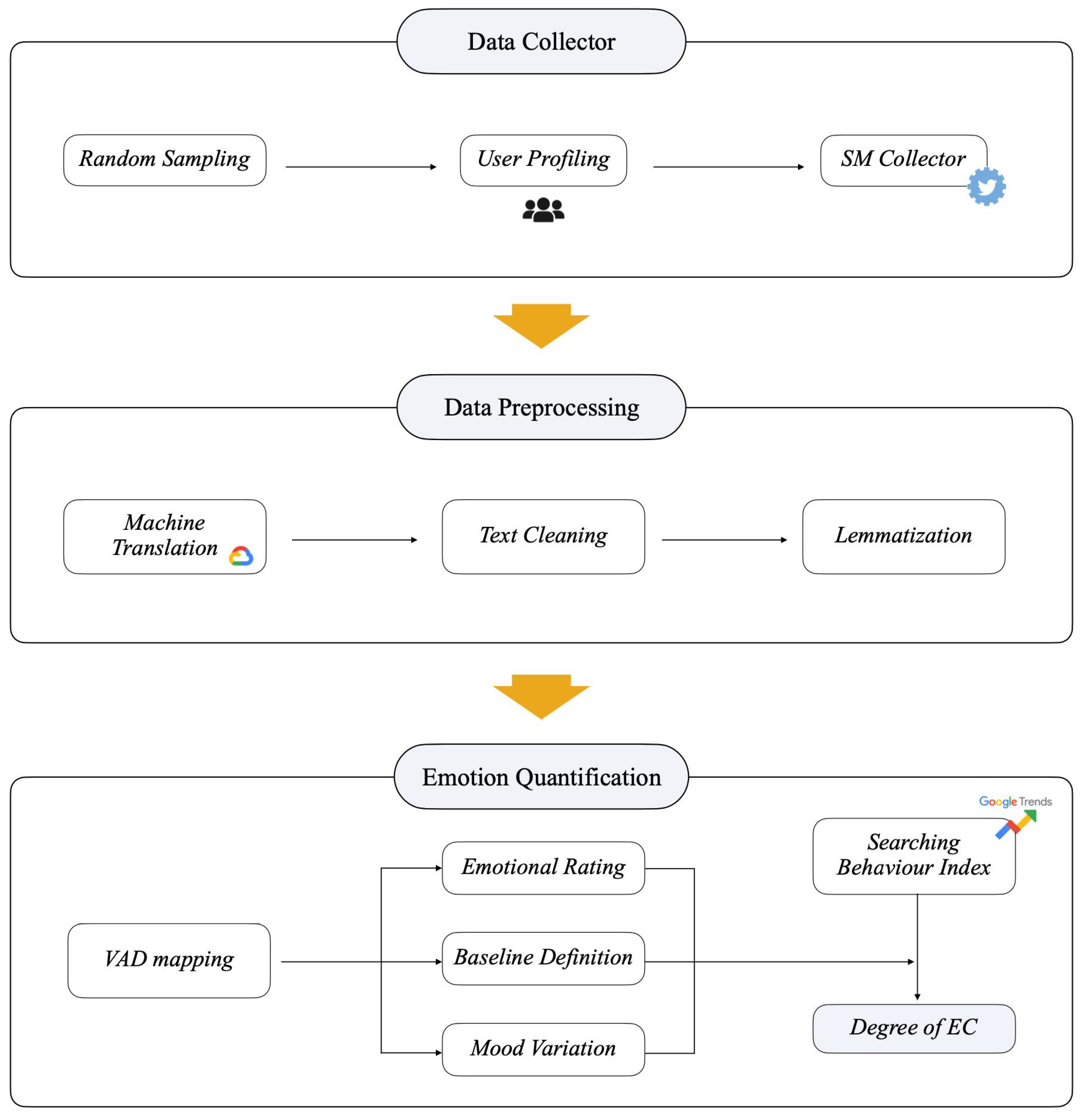
In this section, we will introduce the architecture we build for the development of this case study and explain the different modules involved in the process (Figure 2).
Each of these blocks is defined according to the task they accomplish and will be explained in further detail in the following subsections.
4.1. Data Collector
We must define two main parameters in order to fetch the social interactions that we will need to build our dataset: time period (initial and final time) and location (coordinates and radius).
In order not to fall into a subjective selection, a random search corresponding to a set period is established, with the aim of capturing a first group of potential users to work with. This initial group will serve as the first intuition about the group that we will end up using to subtract social interactions as an object of study.
Once we have the initial harvest, we define a set of filters in order to have a standardized group upon which we could perform our analysis. The filters through which we ran our initial user list are the following:
- User Activity. Minimum rate of interactions per week.
- Account Type. Personal, Organizations, Publicity, etc.
- Join Date. To ensure a comfortable and integrated use of the SMN.
- User Count. Minimum number of users per location.
These conditions can help us define a group of steady, regular active users, whose social profile is adequate to infer useful information from it.
Having built our list of candidates, we proceed to collect a number of interactions from each of the users, attending to the specified parameters for time period and location. A language filter may be used to fetch only certain interactions.
The data collected by our system are publicly available through the Twitter API. Sensitive and potentially identifiable information, such as profile username or tweet content, is automatically encoded for emotional content upon acquisition. Data are analyzed anonymously and aggregated only. Therefore, the individual consent of the users was not required.
4.2. Data Preprocessing
Once the data we will use in our study has been obtained, we will apply a series of NLP techniques [42] to clean and standardize the text. Since we chose to search for social posts in the country’s native language, assuming a greater reach, we must deal with the steps required in order to work with the selected lexicon, which in our case is XANEW. By using an English annotated dictionary, we had two options: either find lexicons for each of the languages we had or translate all posts into English. The main problem of the first option is that, although there exists such annotated dictionaries, they may not be as extensive as XANEW. Therefore, we chose to apply machine translation to all social posts by using Google Translate API (Google Cloud Translate https://cloud.google.com/translate/, accessed on 24 February 2021). The results obtained were manually reviewed in random chunks by native speakers, also assuming the performance offered by this service (Table 2), since a full manual inspection was unrealistic due to the volume of data.
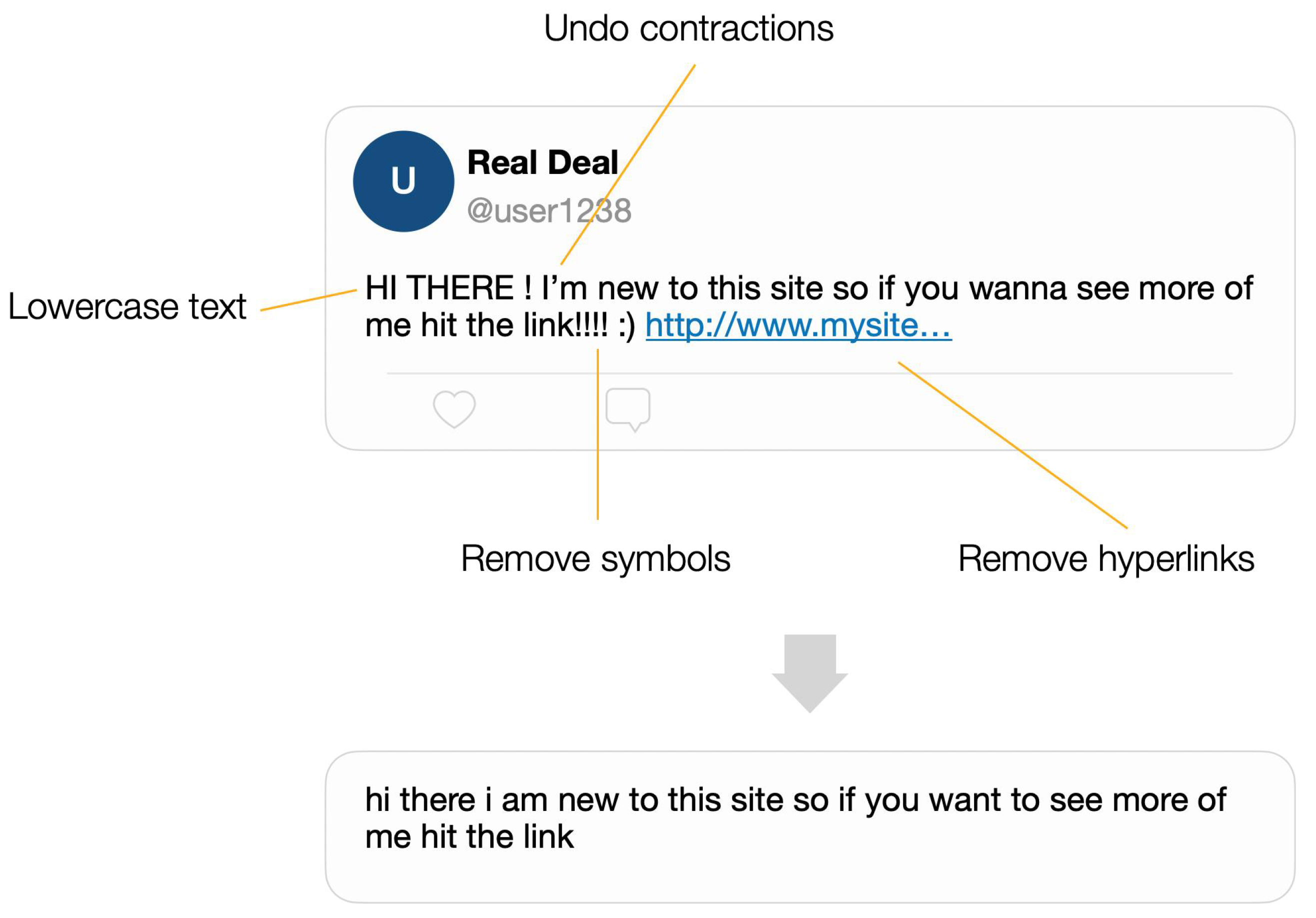
In further steps, we will apply a series of corrections:
- Undo contractions.
- Lowercase text.
- Correct identified misspellings.
- Replacement of consecutive non-ASCII characters and hyperlinks.
- Tokenization of posts.
As we can see in Figure 3, these techniques help us improve the quality of our dataset and remove unnecessary information, such as smilies or hyperlinks.
An additional and important step will apply lemmatization to all tweets, so that we are left with terms that are mappable to our lexicon, aiming to capture a greater range of expressions.
4.3. Emotional Quantification
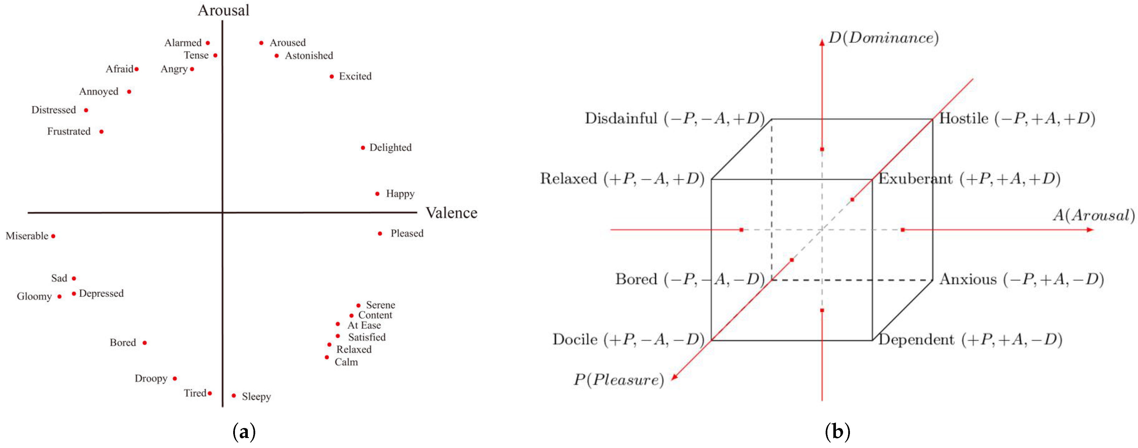
By building and applying our mapping function, and selecting a lexicon, we are able to assign a score to all the interactions from our dataset. Once we do that, we can calculate the values for the Emotional Rating and represent the interactions in the Circumplex Model, (Figure 4a), as well as in the PAD dimensional space (Figure 4b), an essential step to calculate the emotional metrics described in Section 3.1.3. The main difference between the two models shown is the dimensionality: the Circumplex model, firstly developed by Russell, only contemplates two dimensions, while the PAD model, an evolved version, contributes by adding the Dominance dimension and providing a more detailed representation.
Having mapped the VAD values from the selected lexicon, we can calculate the Emotional Rating for all posts of a user, allowing us to obtain such value at a user level by aggregating the VAD values as explained in previous sections. Next, we would be able to obtain the Emotional Baseline and Emotional Charge for each of the users, and therefore measure the distance to specific moods in the PA(D) space, as well as the variation in time from to , where those periods refer to interactions from a specific time frame (i.e., period1 = February-2019, period2 = February-2020). By grouping these results by location, we attain the mood variation at location level. In Table 3, we see a sample of what we work with when calculating the values we need.
On another topic, by establishing a set of terms to analyze their trend, we attain the Searching Behavior Index, having, therefore, the necessary ingredients to calculate the degree of Emotional Concern defined in Equation (15). There is a series of factors that should be taken into consideration when choosing terms for Google Trends in order to ensure a valid analysis. Google Trends is not case sensitive, but plurals or accents might alter the results. When choosing keywords for this search, we encounter two main options to choose from: search term and topic (or disease). While “search term” returns the results that include all keywords including that term, the option “topic” or “disease” captures a wider number of keywords that fall into that category. It is also important noting that “topic” covers the same group of terms that share the same concept in any language, while "search term" would need to be translated to the specific language [39].
5. Experiment Results and Discussion
After applying the method that we have developed, we present in this section the results obtained and we will analyze the conclusions that can be observed from them. The subject we are dealing with is the emotional response of the population against the arrival of COVID-19 during a period comprising the months from February 2019 until October 2019, and February 2020 until October 2020. The reason behind selecting this topic for our study can be summarized into three main ones: (a) It is a relevant subject which still affects our daily lives, (b) it has reached all continents, turning this topic into a global concern, and (c) it is a highly discussed subject for many reasons (counter-measures, mask policies, negationists, etc.). We chose the same period for the previous year in order to establish a baseline on which to measure variations. Using the Twitter Search API, we collected millions of tweets from different European capitals for that time period. In order to harvest geolocated tweets, we specified the coordinates (latitude and longitude) for each of the cities (Berlin, London, Madrid, Rome, Paris, and Warsaw), covering a 20 km radius. The filters through which we ran our initial user list are reflected in Table 4:
We chose these locations as the target for our study based on the fact that, even if all of them belong to the same continent and the European Union, different measures were taken in each place, so we will observe similarities and differences in their reaction to the pandemic. Our Data Collection module contains the six harvesters in charge of building our dataset, based on previously defined criteria. No search terms have been specified, aiming to avoid a bias or polarization of the results, intending, therefore, to observe a general reaction, instead of a focused analysis around a specific topic.
The resulting dataset is made up of more than 5 million tweets, coming from an average of 200 users per city. As we have already explained, these users will be the representative group at the geographical level for each city and country. We want to indicate the fact that no language filters have been imposed on the extraction of tweets, assuming that the vast majority of users would interact in the native language. Therefore, we used the Machine Translation service from Google Cloud API to translate all interactions into English, and the spaCy (spaCy https://spacy.io/, accessed on 26 February 2021) library to carry out the necessary lemmatization.
To calculate the Searching Behavior Index related to the subject of the COVID-19 pandemic, we chose the terms presented in Table 5. Each of these terms is language-specific for each country, following the assumption of a native-language search for each of the locations.
To the best of our knowledge, there has not been any similar study that we can use as a comparison of ground truth. However, we extend the work done in the past [19], which covered the quantification of the Emotional Impact of certain events on different locations, by introducing the degree of Emotional Concern, which reflects the emotional response as the variation in people’s concern based on values of valence, arousal, and dominance, and their relation to searching behavior on Google. We also extend our contribution in this work by expanding our criteria in data gathering, meaning that, instead of monitoring specific keywords or hashtags, we take into account unbiased tweets, so we not only can capture how people react to the pandemic but also how they deal with their daily lives in general.
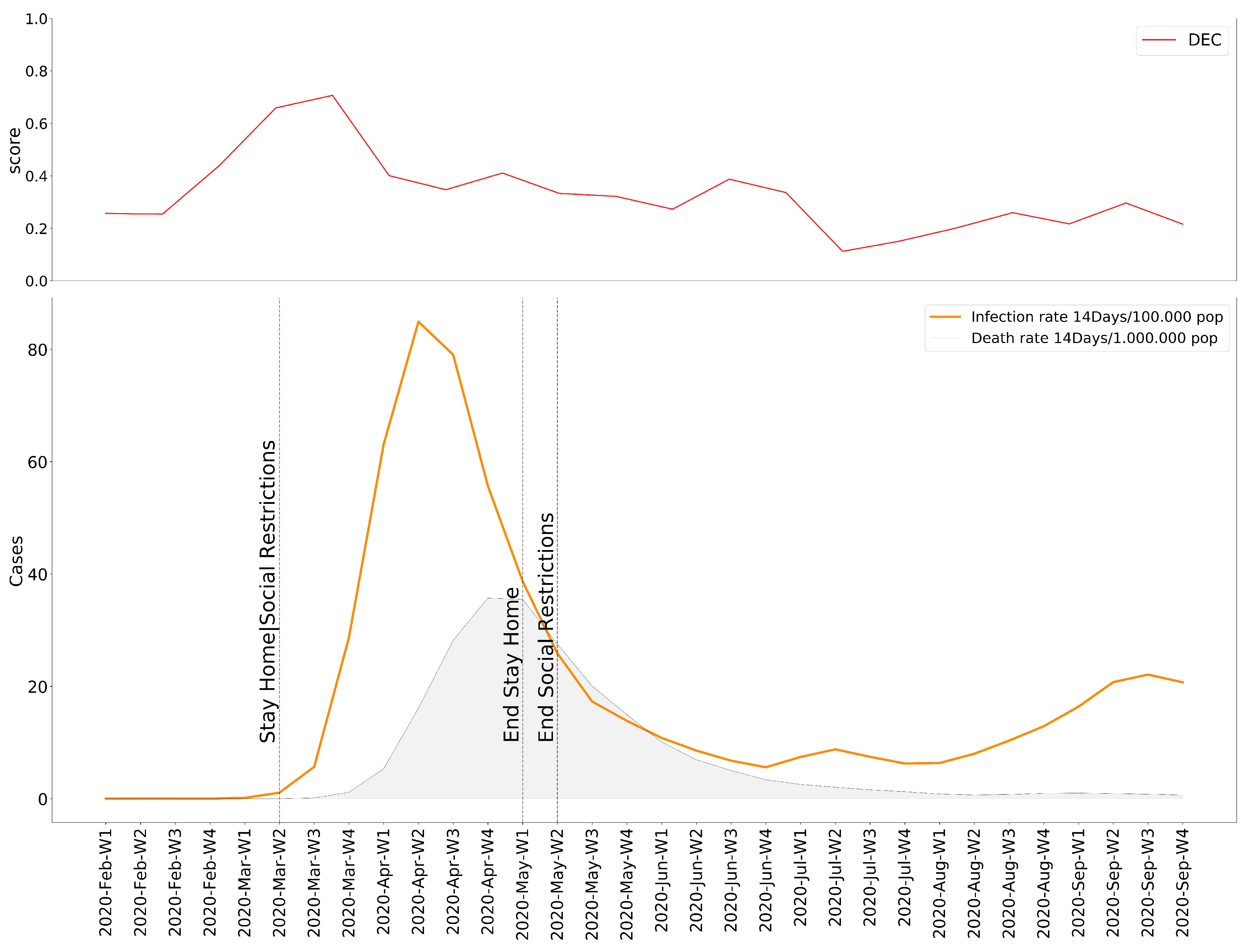
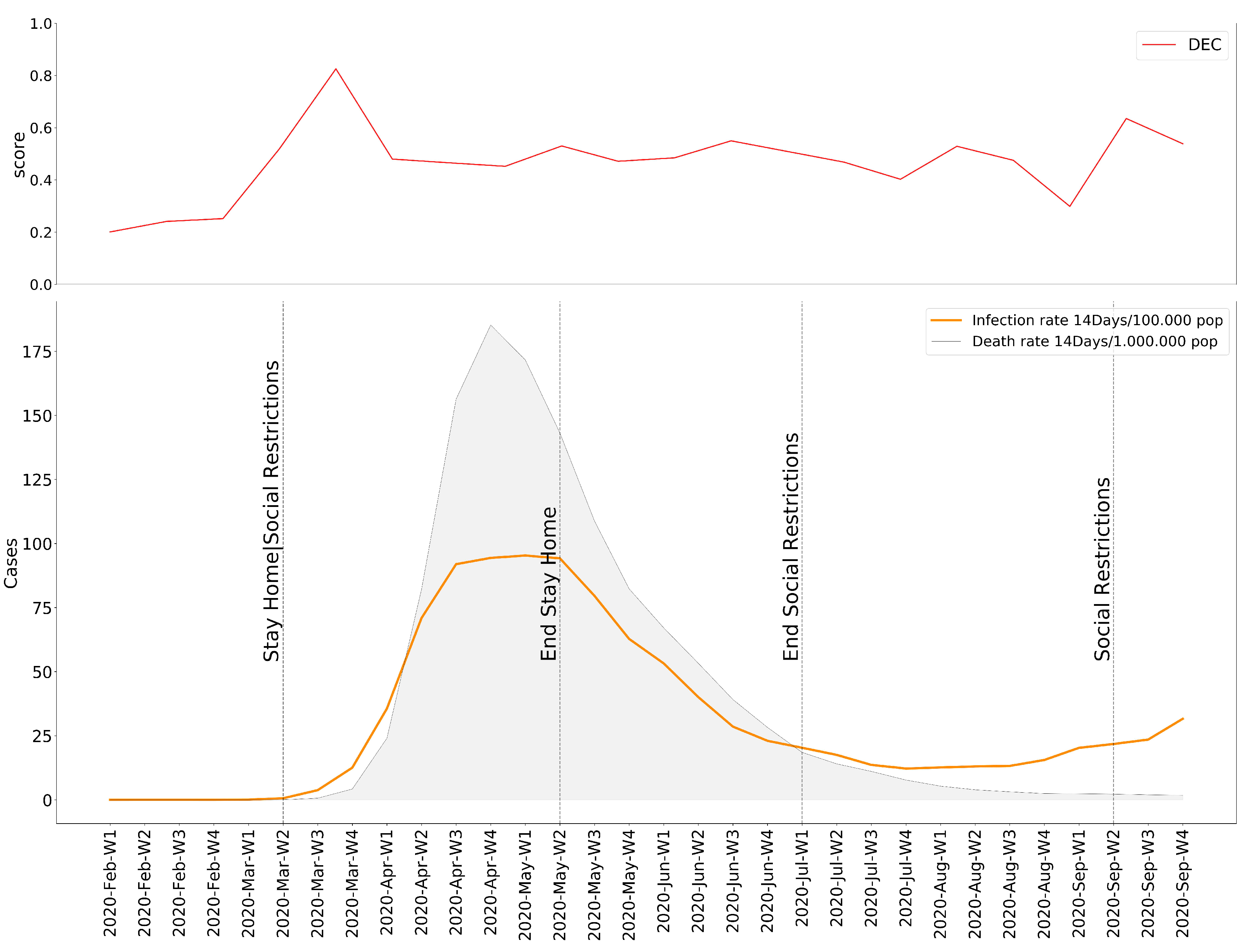
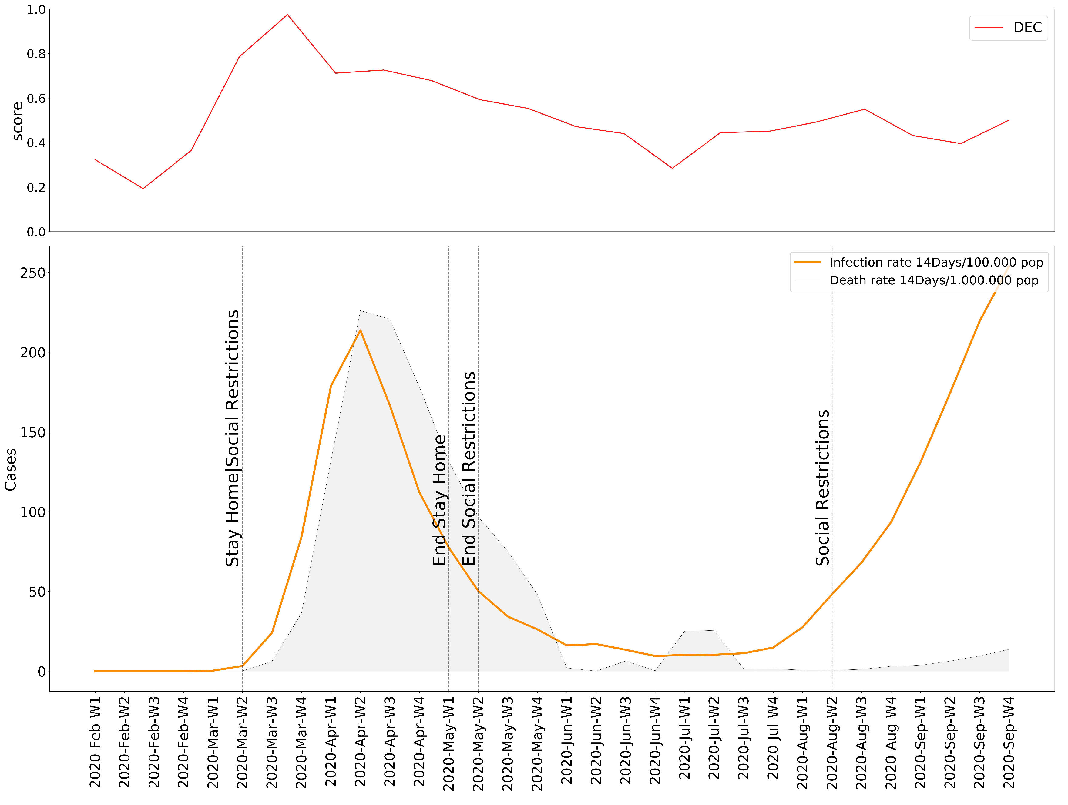
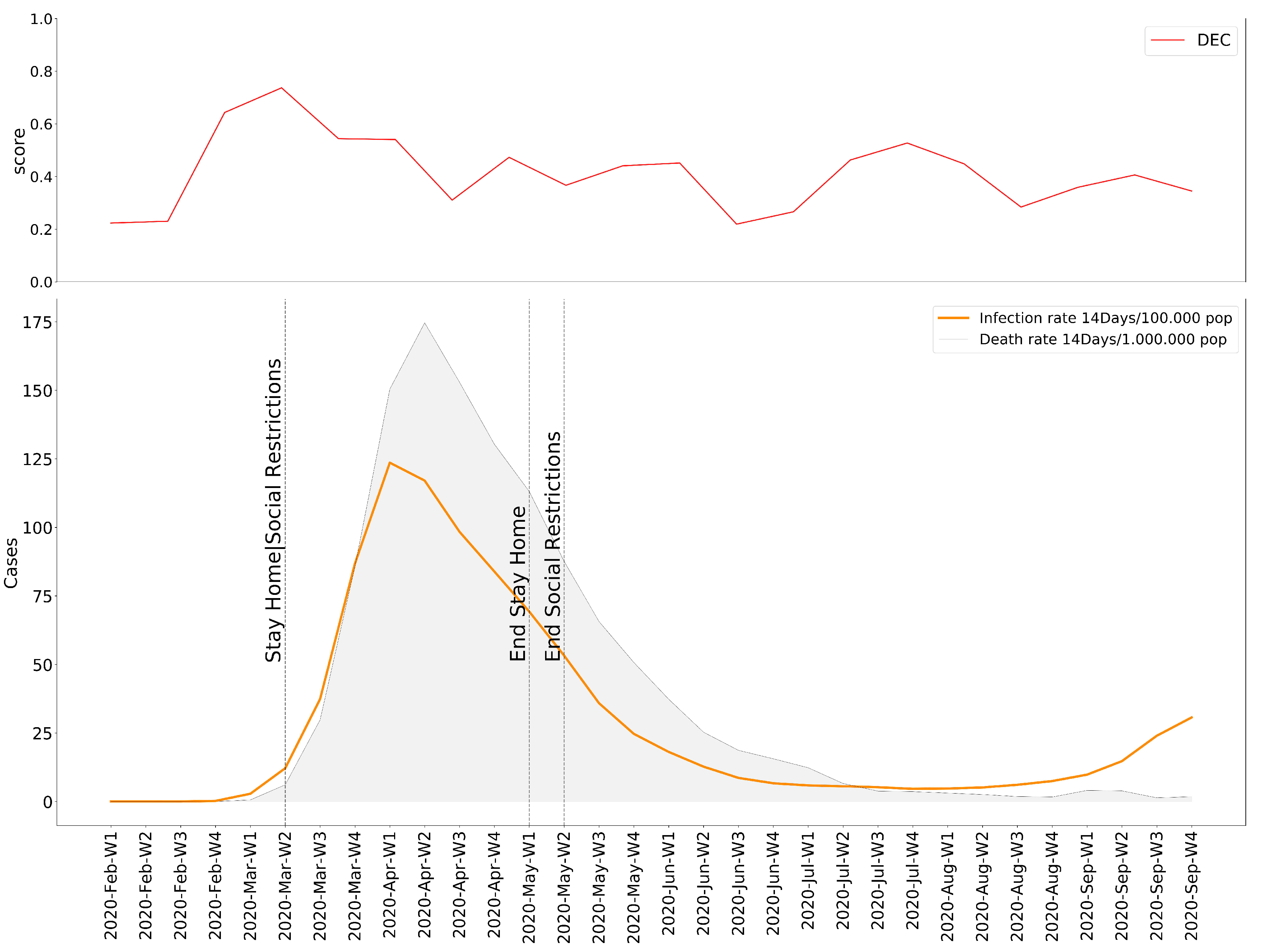
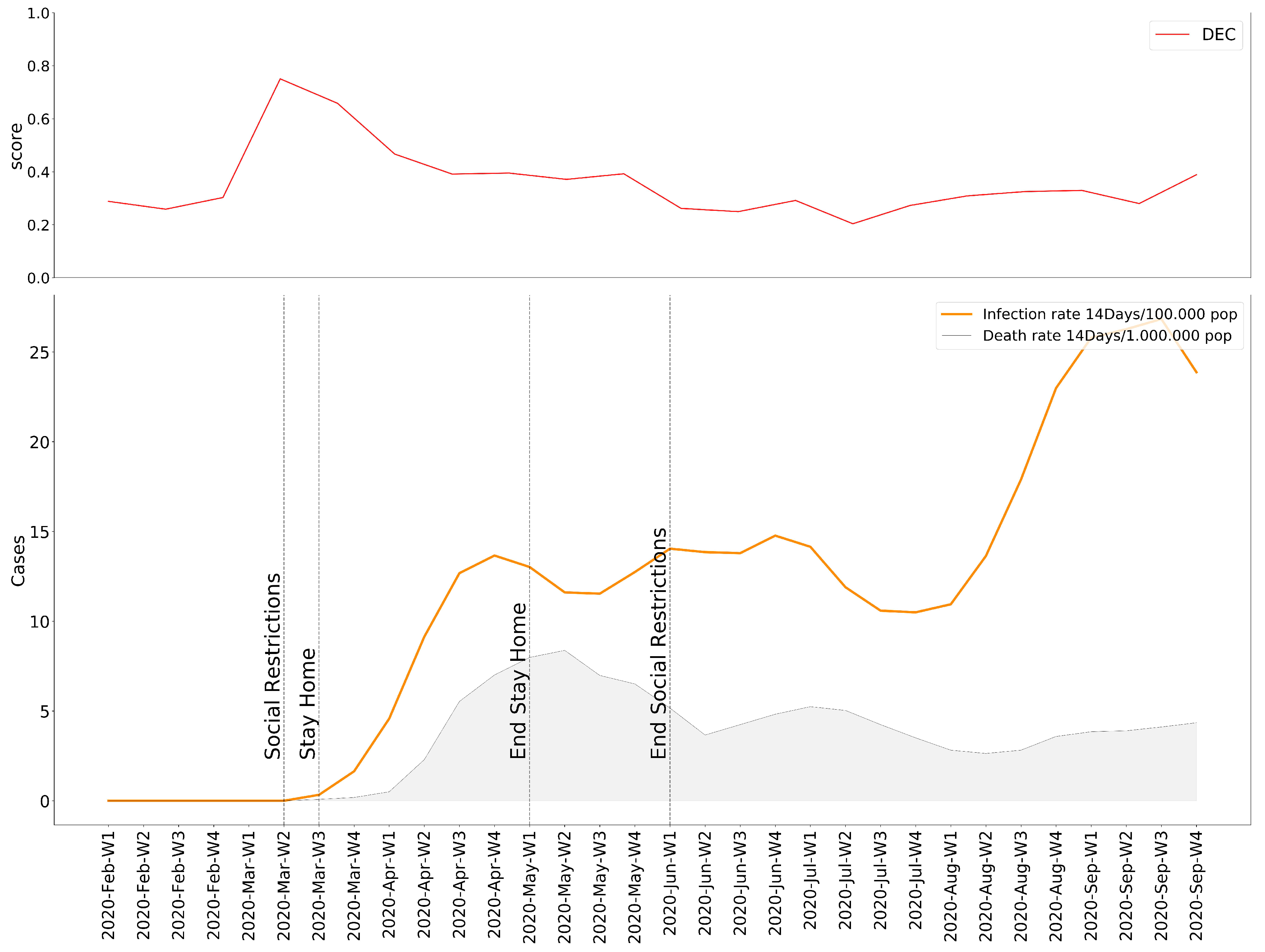
Once the necessary operations have been executed, we possess values for the Emotional Rating, Emotional Impact, and Emotional Baseline; all the ingredients we need to expose our results. Based on these variables, we present our observations as the individual variation of the degree of Emotional Concern as well as the 15 selected moods. In order to follow the evolution of the pandemic, we decided to help ourselves with the data of the accumulated incidence of 14 days of COVID-19 cases and deaths for each country [44], plus their respective response measures [45]. The results obtained in this experiment lead to the conclusion that, for most cities, the onset of the pandemic is received with a clear negative reaction—an increase in moods with a higher rate of displeasure in the Circumplex model (Figure 5, Figure 6, Figure 7, Figure 8, Figure 9 and Figure 10), associated with the exponential increase in cases nationwide. The degree of emotional concern (DEC) thus reflects an increase in concern about this growing number of infections. We could speak of a certain causality concerning DEC and the imposition of restrictive countermeasures on social activities and mobility, as a response to the gravity of the situation. At first glance, it is evident that the emotional response is not the same in all countries: we find similarities in Berlin, London, Madrid, and Warsaw (Figure 5, Figure 6, Figure 7, Figure 8, Figure 9 and Figure 10), where the DEC evolves with a decreasing trend concerning the initial peak, while in Rome and Paris that variation is not so tangible (Figure 8 and Figure 9).
As we can see, in every location, we can find a growing trend in the degree of Emotional Concern corresponding to a first reaction. It was on 11 March when WHO declared COVID-19 a global pandemic, and governments started taking action around the same time, impacting the daily lives of the population. This came to be reflected in social interactions, for example, by considering mood variations in Madrid (Figure 11), people are feeling more nervous, tense, and upset than the previous year. We can find a strong correlation between our results and those resulting from previous studies that concluded an increase in low valence emotions, such as anger, anxious, or tense [46].
However, in all six locations, the DEC begins decreasing after this first peak. We find a steady decrease rate in some cities like Warsaw, where the infection and death rate of the country is much lower than the rest. On the other hand, Rome presents an unstable evolution of the DEC. Focusing again on Madrid, it is noticeable how, given the number of infections and deaths, the DEC still falls significantly after its summit, and even when a new wave of infections begins, the DEC response is not quite the same as in the beginning.
This concurs with findings from other authors, where social media monitoring revealed an increase in emotions such as anger, fear, and anxiety soon after the beginning of the pandemic [46]. Psychology also shows that people tend to feel anxious and unsafe in response to environment changes, especially in the case of disease outbreaks, when the cause or progression of the disease and outcomes are unclear, rumors grow and close-minded attitudes eventuate [47]. In most countries, during the first phase of the pandemic, rates for depression, anxiety, and insomnia increased significantly in comparison to previous years, while these rates noticeably decreased as time passed since the beginning of the pandemic [48,49,50]. This observation may lead us to argue that, in general terms, a decrease in DEC means an adaptation or getting accustomed to living in such a tragic situation, where, although there is an increase in the cumulative incidence of COVID-19 cases, the response, if any, is not so negative. This aspect of acquired indifference has been studied numerous times in the field of human psychology, associated with the need for survival and resilience in the face of extremely aversive events [51]. Other authors already demonstrated that we not only become numb to the significance of increasing numbers, but our compassion can actually fade or collapse overall as numbers increase [52].
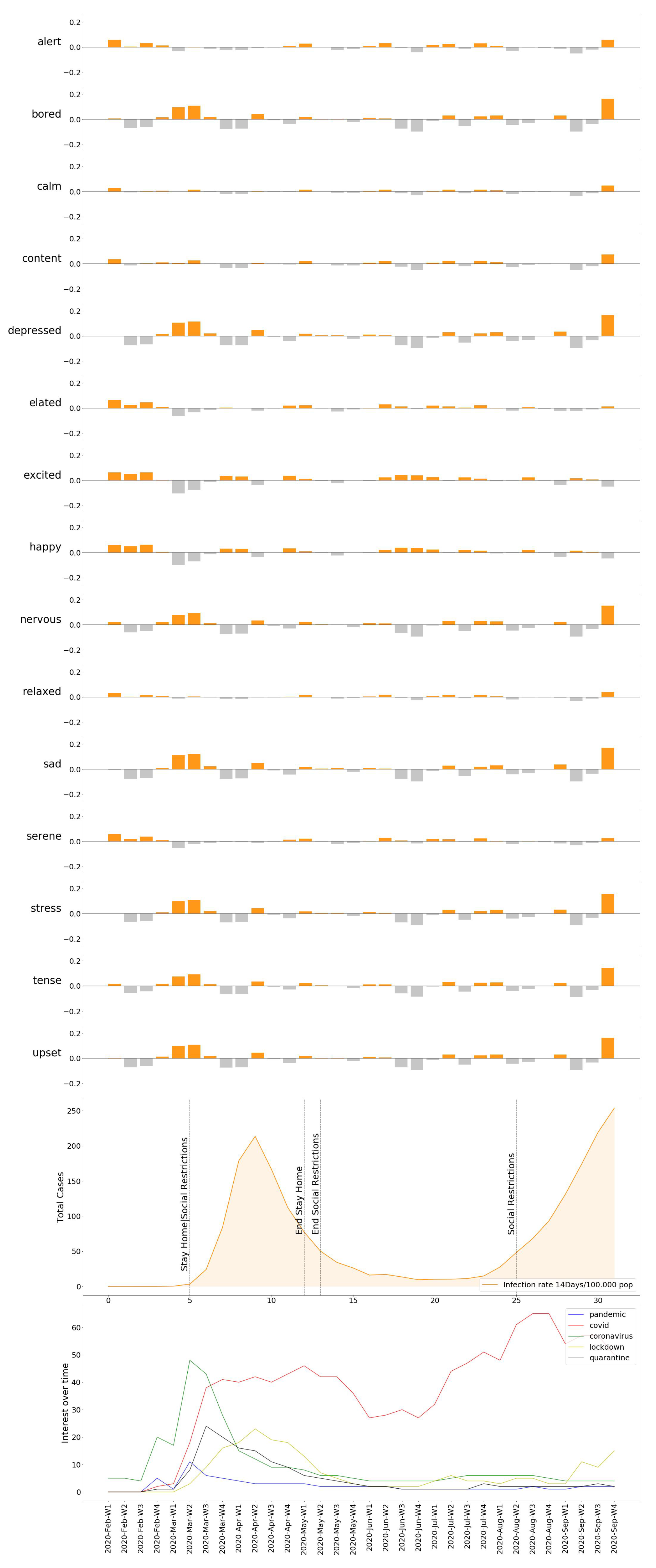
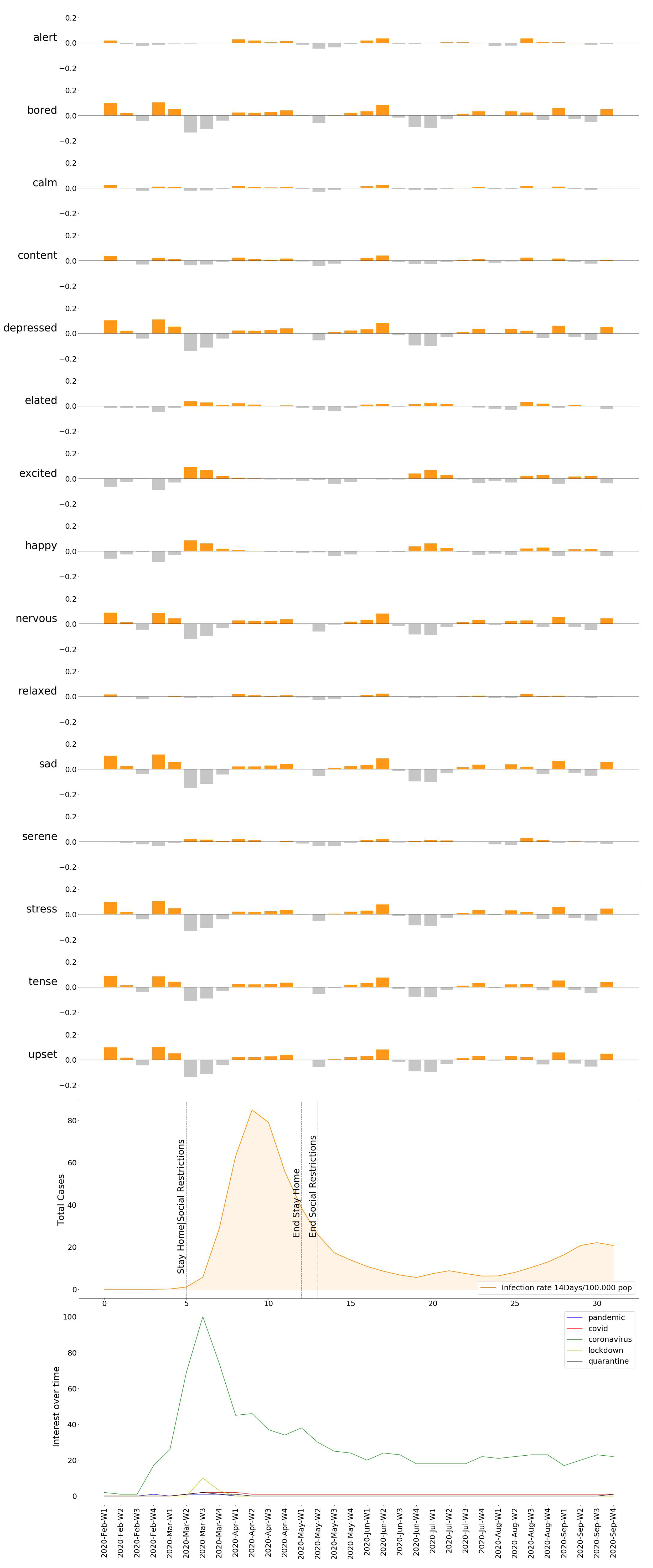
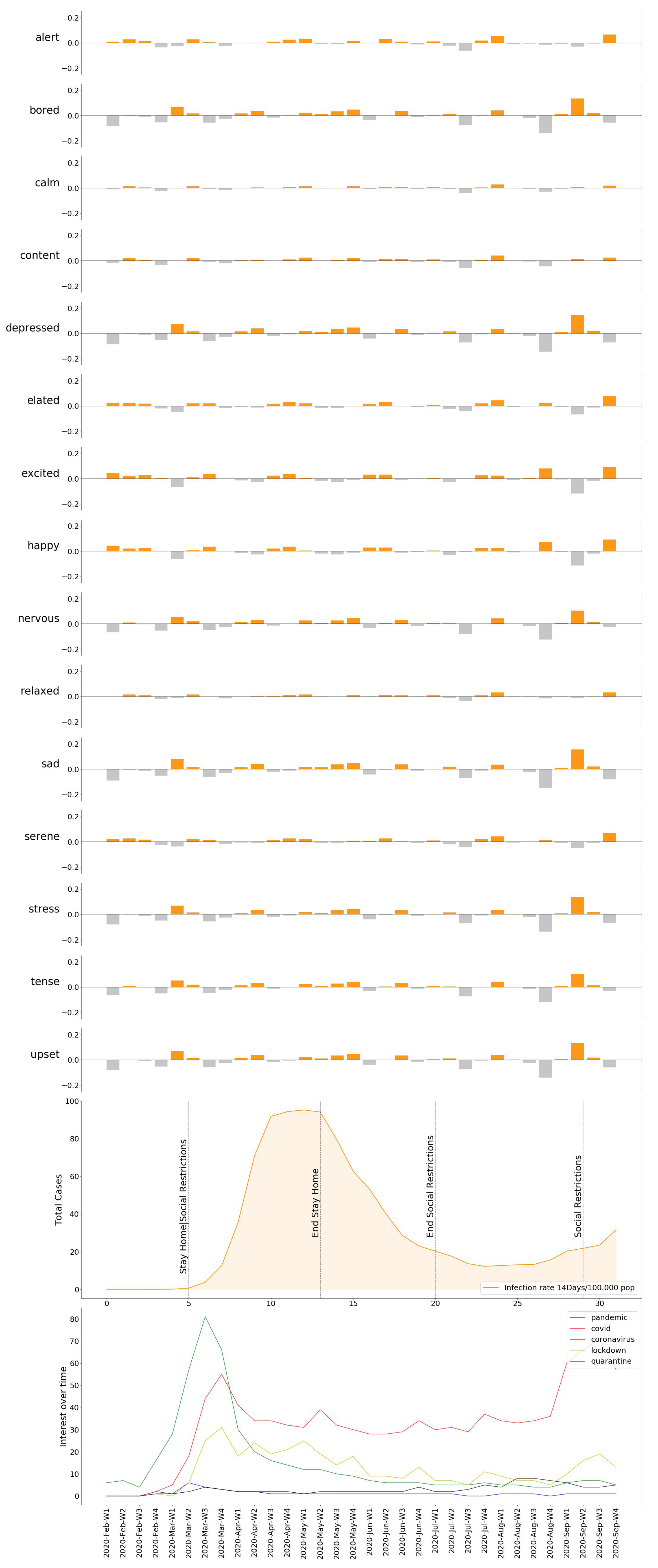
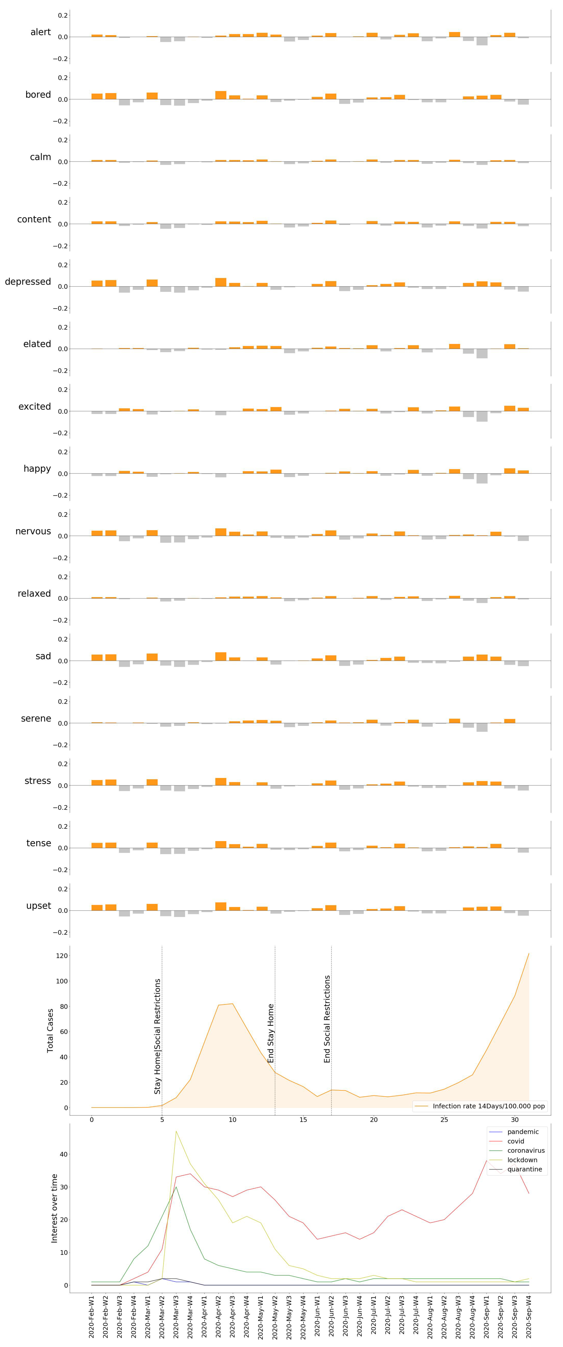
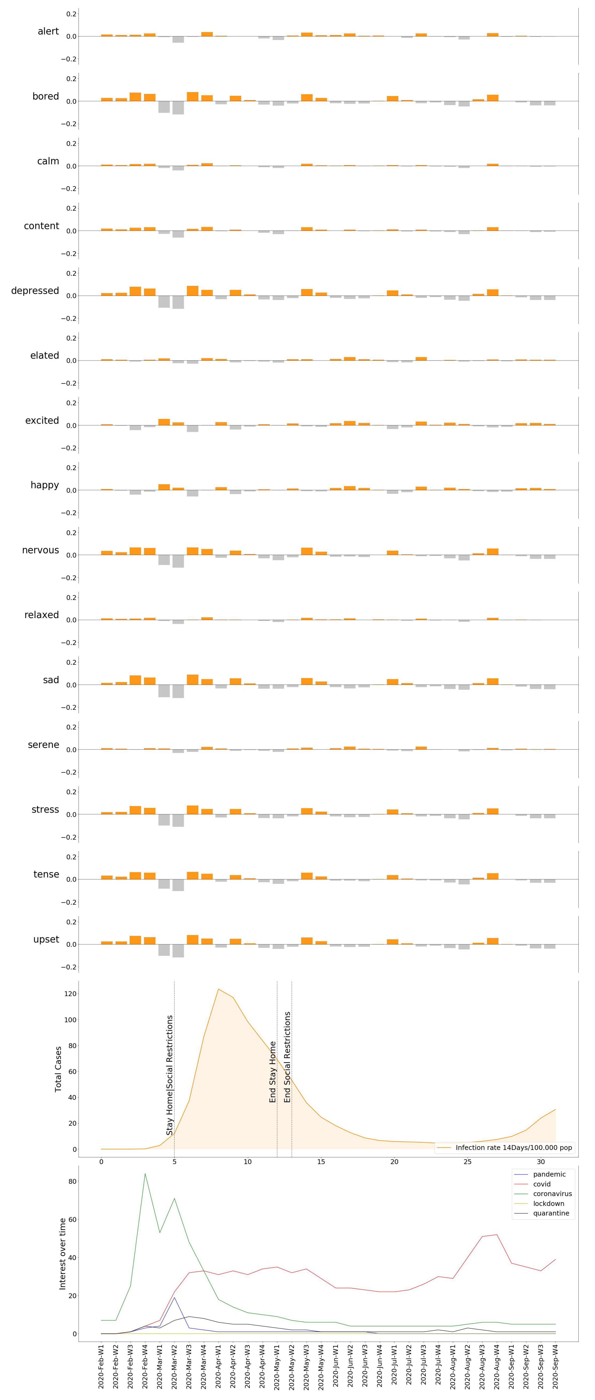
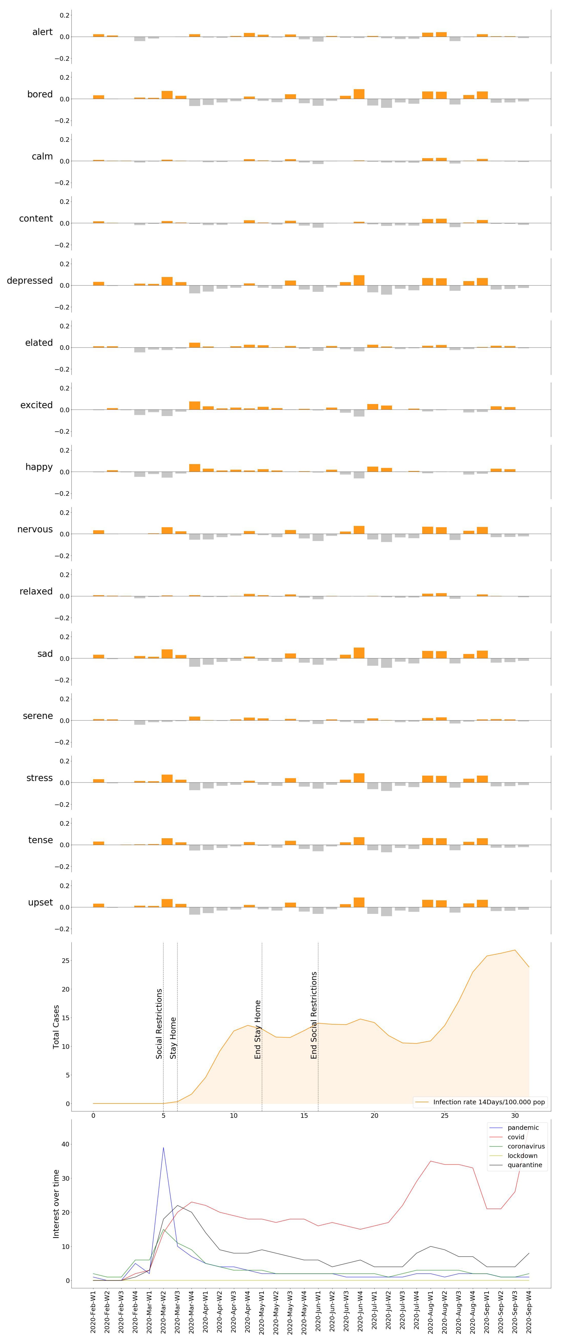
Similarly, we can see how the emotional response spreads over the individual moods in Figure 12, Figure 13, Figure 14, Figure 15 and Figure 16, providing us with a more detailed insight on the variation of specific emotions over that period of time.
It is important to emphasize the reach, scope, and limitations of our method: we make use of the aggregated opinions of a collective, which we consider representative for a whole location, collected for two periods of time, in order to create a new method to quantify and calculate an index that can measure the emotional concern of the population. The first assumption we make is choosing the selected target group as a representative for the whole population. By choosing a specific timeframe, we are aware of possible mood changes that we do not capture, and this could directly influence the results we present. Our Social Media analysis assumes that the total population studied in this work expresses their complete and absolute opinion via these networks, thus, even contemplating the possibility that people use Twitter to communicate only certain emotions (i.e., angry tweets, hate speech, etc.), we dismiss this case, as the scientific community provides sufficient support to utilize this practice [11,12,19,34,36,40,46]. We establish our criteria to obtain good candidates in all transparency, aiming to build an unbiased dataset.
Secondly, we build our method based on a lexicon. We decided to choose this approach instead of more recent architectures based on the format of the data we work with: opinions expressed in a few words or sentences. Although current state-of-the-art architectures provide exceptional results in text classification, as classes increase, their performance decrease. Adding to this, our resources did not allow for a labeled dataset upon which to train such models. Accepting the limitations of a lexicon, it provides valid representations of its aggregated values on PA(D) models, as shown by previous works from other authors [34,35,46]. On top of that, emotion labeling and classification still is a fuzzy field in psychology, existing no consensus over a global emotion model, thus choosing a specific approach bears the exclusion of different methods. Nevertheless, being aware of the possible limitations of our method, we establish that the scope of this study is to build the degree of Emotional Concern based on two relevant factors: Emotional Impact and Searching Behavior.
6. Conclusions
In this paper, we deal with the subject of measuring the population’s concern with respect to an event prolonged in time. We chose COVID-19 as the subject for our study based on the relevance and global impact it has had. Therefore, we present to the community our very own method to build the degree of Emotional Concern, explaining our approach at modeling and quantifying the emotional response to the global pandemic based on data gathered from different geotagged locations using Social Media and dimensional models of emotion. To achieve that, we gathered geolocated data from six different locations over the period of eight months, during the course of two years. Presenting the concepts of Emotional Baseline, Emotional Impact, Mood Variation, and the novel definition of Searching Behavior Index, we calculate the degree of Emotional Concern for each location as the result of a normalized, weighted aggregation between the Mood Variation around the emotion concerned and the .
In order to calculate the Emotional Rating, necessary to calculate the Emotional Charge, Emotional Baseline, etc., we rely on the dimensional model PAD for emotion classification introduced by Russell, mapping the social interactions on the tridimensional space making use of the eXtended Affective Norms for English Words, which gives VAD values to a set of nearly 14,000 words. This allows us to measure the closeness—or distance—of social interaction to a specific mood, such as tense or excited, which we perform for the 15 named moods introduced in Table 1.
Although Social Media is a growing industry, not all the population, in terms of age range, is using it and, therefore, not all opinions are reflected. This is what drove us to include the Searching Behavior as a parameter when calculating the degree of Emotional Concern, so those who are not represented in the interactions we collected can still be captured by this concept, which holds a much bigger audience. There is solid proof in the field supporting the use of Google Trends as a tool to gain insights into the population’s interest [53], behavior with respect to an event [38] and even emotional outcome derived from the online search [54]. This past research helps us substantiate the combination with the searching index we developed with the mood variation, in order to create our DEC, which is the novelty we present in this work.
Once the DEC for all locations is obtained, we displayed the results found compared against the pandemic evolution (infection rate, death rate, government measures), in order to observe and comprehend its progress. The DEC in all locations reached its peak when the spread of the virus acquired an exponential trend. From that point on, four cities showed a similar evolution, which is a progressive decrease in the DEC. More detailed insights are provided in Figure 12, Figure 13, Figure 14, Figure 15 and Figure 16, where named mood variations are displayed. These figures show in a more detailed manner how predominant negative emotions arise as a reaction to countermeasures such as lockdown and social restrictions, while they start fading away, being replaced by more neutral and even strong positive emotions once these restrictions are lifted, regardless of the infection rate.
Our results shed some light into the field of human behavior and psychology, by bringing to the community a long-term response to a tragic event. We find that populations across countries react in quite similar ways after being exposed to similar restrictions. The work we present here can be used in many scenarios: as we suggested, the notable decrease in people’s preoccupation could be linked to human resilience or adaptation to prolonged situations, even if they are catastrophic. This research could be continued by exploring other locations and for longer periods of time: we used as a baseline the previous year, thus extending our range to the previous years might give us a more rigorous measure. Similarly, including additional parameters, such as economic impact, solidarity evolution, or hospital data could give us a better understanding of which locations coped best with the situation and what the drivers were. It can also be applied to other topics, such as people’s reactions to melting glaciers, global warming, water crisis, or political conflicts. It would also be interesting to consider how fake news affected and polarized people’s opinion in this specific scenario, where negationists and anti-vaxxers played a significant role.
Author Contributions
Both authors have contributed in the same way to this paper. All authors have read and agreed to the published version of the manuscript.
Funding
This research received no external funding.
Conflicts of Interest
The authors declare no conflict of interest.
References
- WHO Naming the Coronavirus Disease (COVID-19) and the Virus that Causes It; WHO: Geneva, Switzerland, 2020.
- Cucinotta, D.; Vanelli, M. WHO declares COVID-19 a pandemic. Acta Bio Med. Atenei Parm. 2020, 91, 157. [Google Scholar]
- Tirachini, A.; Cats, O. COVID-19 and public transportation: Current assessment, prospects, and research needs. J. Public Transp. 2020, 22, 1. [Google Scholar] [CrossRef]
- Pak, A.; Adegboye, O.A.; Adekunle, A.I.; Rahman, K.M.; McBryde, E.S.; Eisen, D.P. Economic consequences of the COVID-19 outbreak: The need for epidemic preparedness. Front. Public Health 2020, 8, 241. [Google Scholar] [CrossRef] [PubMed]
- WHO Impact of COVID-19 on People’s Livelihoods, Their Health and Our Food Systems; WHO: Geneva, Switzerland, 2020.
- European Commission. Timeline of EU Action; European Commission: Brussels, Belgium, 2021. [Google Scholar]
- YouGov International. Personal Impacts of Coronavirus; YouGov International: London, UK, 2020. [Google Scholar]
- Barrett, L.F. How Emotions Are Made: The Secret Life of the Brain; Houghton Mifflin Harcourt: Boston, MA, USA, 2017. [Google Scholar]
- Ekman, P. Basic emotions. In Handbook of Cognition and Emotion; John Wiley & Sons: Hoboken, NJ, USA, 1999; Volume 98, p. 16. [Google Scholar]
- European Union Internet Users, Population and Facebook Statistics. 2021. Available online: https://www.internetworldstats.com/stats9.htm (accessed on 10 March 2021).
- Lathi, K. Social Media as a Data Source. 2016. Available online: https://elicitinsights.com/blog/social-media-as-a-data-source/ (accessed on 15 March 2021).
- Pak, A.; Paroubek, P. Twitter as a Corpus for Sentiment Analysis and Opinion Mining. In Proceedings of the Seventh International Conference on Language Resources and Evaluation (LREC’10), Valletta, Malta, 17–23 May 2010; European Language Resources Association (ELRA): Valletta, Malta, 2010. [Google Scholar]
- Iqbal, M. Twitter MAU, Q1 2010–Q1 2019, Millions; Business of Apps: London, UK, 2020. [Google Scholar]
- Aggarwal, C.C. Machine Learning for Text; Springer: Berlin/Heidelberg, Germany, 2018. [Google Scholar]
- Vaswani, A.; Shazeer, N.; Parmar, N.; Uszkoreit, J.; Jones, L.; Gomez, A.N.; Kaiser, L.; Polosukhin, I. Attention is all you need. arXiv 2017, arXiv:1706.03762. [Google Scholar]
- Lample, G.; Conneau, A. Cross-lingual language model pretraining. arXiv 2019, arXiv:1901.07291. [Google Scholar]
- Lewis, M.; Liu, Y.; Goyal, N.; Ghazvininejad, M.; Mohamed, A.; Levy, O.; Stoyanov, V.; Zettlemoyer, L. Bart: Denoising sequence-to-sequence pre-training for natural language generation, translation, and comprehension. arXiv 2019, arXiv:1910.13461. [Google Scholar]
- Warriner, A.B.; Kuperman, V.; Brysbaert, M. Norms of valence, arousal, and dominance for 13,915 English lemmas. Behav. Res. Methods 2013, 45, 1191–1207. [Google Scholar] [CrossRef] [Green Version]
- Bernabé-Moreno, J.; Tejeda-Lorente, A.; Porcel, C.; Fujita, H.; Herrera-Viedma, E. Quantifying the emotional impact of events on locations with social media. Knowl. Based Syst. 2018, 146, 44–57. [Google Scholar] [CrossRef]
- Galea, S.; Merchant, R.M.; Lurie, N. The mental health consequences of COVID-19 and physical distancing: The need for prevention and early intervention. JAMA Intern. Med. 2020, 180, 817–818. [Google Scholar] [CrossRef] [Green Version]
- Centers for Disease Control and Prevention. Risk for COVID-19 Infection, Hospitalization, and Death By Age Group; Centers for Disease Contri and Prevention: Atlanta, GA, USA, 2021. [Google Scholar]
- Iqbal, M. Global Twitter Users by Age and Gender; Business of Apps: London, UK, 2020. [Google Scholar]
- Ripberger, J.T. Capturing curiosity: Using internet search trends to measure public attentiveness. Policy Stud. J. 2011, 39, 239–259. [Google Scholar] [CrossRef]
- Higgins, T.S.; Wu, A.W.; Sharma, D.; Illing, E.A.; Rubel, K.; Ting, J.Y.; Alliance, S.F. Correlations of online search engine trends with coronavirus disease (COVID-19) incidence: Infodemiology study. JMIR Public Health Surveill. 2020, 6, e19702. [Google Scholar] [CrossRef]
- Myers, D.G. Psychology, 7th ed.; Worth: New York, NY, USA, 2004. [Google Scholar]
- Izard, C.E. Human Emotions; Springer Science & Business Media: Berlin/Heidelberg, Germany, 2013. [Google Scholar]
- Jung, C.G. Psychological Types; Routledge: London, UK, 2014. [Google Scholar]
- Russell, J.A. A circumplex model of affect. J. Personal. Soc. Psychol. 1980, 39, 1161. [Google Scholar] [CrossRef]
- Mehrabian, A. Pleasure-arousal-dominance: A general framework for describing and measuring individual differences in temperament. Curr. Psychol. 1996, 14, 261–292. [Google Scholar] [CrossRef]
- Gross, J.J. Handbook of Emotion Regulation; Guilford Publications: New York, NY, USA, 2013. [Google Scholar]
- Stadthagen-Gonzalez, H.; Imbault, C.; Sánchez, M.A.P.; Brysbaert, M. Norms of valence and arousal for 14,031 Spanish words. Behav. Res. Methods 2017, 49, 111–123. [Google Scholar] [CrossRef] [PubMed] [Green Version]
- Schmidtke, D.S.; Schröder, T.; Jacobs, A.M.; Conrad, M. ANGST: Affective norms for German sentiment terms, derived from the affective norms for English words. Behav. Res. Methods 2014, 46, 1108–1118. [Google Scholar] [CrossRef]
- Bravo-Marquez, F.; Mendoza, M.; Poblete, B. Combining strengths, emotions and polarities for boosting twitter sentiment analysis. In Proceedings of the Second International Workshop on Issues of Sentiment Discovery and Opinion Mining, Chicago, IL, USA, 11 August 2013; pp. 1–9. [Google Scholar]
- Larsen, M.E.; Boonstra, T.W.; Batterham, P.J.; O’Dea, B.; Paris, C.; Christensen, H. We feel: Mapping emotion on Twitter. IEEE J. Biomed. Health Inform. 2015, 19, 1246–1252. [Google Scholar] [CrossRef] [PubMed]
- Preoţiuc-Pietro, D.; Schwartz, H.A.; Park, G.; Eichstaedt, J.; Kern, M.; Ungar, L.; Shulman, E. Modelling Valence and Arousal in Facebook posts. In Proceedings of the 7th Workshop on Computational Approaches to Subjectivity, Sentiment and Social Media Analysis, San Diego, CA, USA, 16 June 2016; Association for Computational Linguistics: San Diego, CA, USA, 2016; pp. 9–15. [Google Scholar] [CrossRef]
- Imran, A.S.; Daudpota, S.M.; Kastrati, Z.; Batra, R. Cross-cultural polarity and emotion detection using sentiment analysis and deep learning on COVID-19 related tweets. IEEE Access 2020, 8, 181074–181090. [Google Scholar] [CrossRef]
- Siliverstovs, B.; Wochner, D.S. Google Trends and reality: Do the proportions match?: Appraising the informational value of online search behavior: Evidence from Swiss tourism regions. J. Econ. Behav. Organ. 2018, 145, 1–23. [Google Scholar] [CrossRef]
- Preis, T.; Moat, H.S.; Stanley, H.E. Quantifying trading behavior in financial markets using Google Trends. Sci. Rep. 2013, 3, 1–6. [Google Scholar] [CrossRef] [Green Version]
- Mavragani, A.; Ochoa, G. Google Trends in infodemiology and infoveillance: Methodology framework. JMIR Public Health Surveill. 2019, 5, e13439. [Google Scholar] [CrossRef] [Green Version]
- Bernabé-Moreno, J.; Tejeda-Lorente, A.; Porcel, C.; Fujita, H.; Herrera-Viedma, E. Emotional profiling of locations based on social media. Procedia Comput. Sci. 2015, 55, 960–969. [Google Scholar] [CrossRef] [Green Version]
- Posner, J.; Russell, J.A.; Peterson, B.S. The circumplex model of affect: An integrative approach to affective neuroscience, cognitive development, and psychopathology. Dev. Psychopathol. 2005, 17, 715. [Google Scholar] [CrossRef] [PubMed]
- Uysal, A.K.; Gunal, S. The impact of preprocessing on text classification. Inf. Process. Manag. 2014, 50, 104–112. [Google Scholar] [CrossRef]
- Aiken, M. An updated evaluation of Google Translate accuracy. Stud. Linguist. Lit. 2019, 3, 253–260. [Google Scholar] [CrossRef] [Green Version]
- European Centre for Disease Prevention and Control. COVID-19 Datasets; European Centre for Disease Prevention and Control: Solna, Switzerland, 2021. [Google Scholar]
- European Centre for Disease Prevention and Control. Data on 14-Day Notification Rate of New COVID-19 Cases and Deaths; European Centre for Disease Prevention and Control: Solna, Switzerland, 2021. [Google Scholar]
- Stella, M.; Restocchi, V.; De Deyne, S. # lockdown: Network-enhanced emotional profiling in the time of Covid-19. Big Data Cogn. Comput. 2020, 4, 14. [Google Scholar]
- Usher, K.; Durkin, J.; Bhullar, N. The COVID-19 pandemic and mental health impacts. Int. J. Ment. Health Nurs. 2020, 29, 315. [Google Scholar] [CrossRef] [PubMed] [Green Version]
- Mingote, L.R. COVID-19 y Salud Mental: Más Ansiolíticos, Más Llamadas al 061 y Pocos Psicólogos | lamarea.com. 2020. Available online: https://www.lamarea.com/2021/02/05/covid-19-y-salud-mental-mas-ansioliticos-mas-llamadas-al-061-y-pocos-psicologos/ (accessed on 20 March 2021).
- Fancourt, D.; Steptoe, A.; Bu, F. Trajectories of anxiety and depressive symptoms during enforced isolation due to COVID-19 in England: A longitudinal observational study. Lancet Psychiatry 2021, 8, 141–149. [Google Scholar] [CrossRef]
- Essadek, A.; Rabeyron, T. Mental health of French students during the Covid-19 pandemic. J. Affect. Disord. 2020, 277, 392–393. [Google Scholar] [CrossRef]
- Bonanno, G.A. Loss, trauma, and human resilience: Have we underestimated the human capacity to thrive after extremely aversive events? Am. Psychol. 2004, 59, 20. [Google Scholar] [CrossRef] [Green Version]
- Västfjäll, D.; Slovic, P.; Mayorga, M.; Peters, E. Compassion fade: Affect and charity are greatest for a single child in need. PLoS ONE 2014, 9, e100115. [Google Scholar] [CrossRef] [Green Version]
- Choi, H.; Varian, H. Predicting the present with Google Trends. Econ. Rec. 2012, 88, 2–9. [Google Scholar] [CrossRef]
- Flavián-Blanco, C.; Gurrea-Sarasa, R.; Orús-Sanclemente, C. Analyzing the emotional outcomes of the online search behavior with search engines. Comput. Hum. Behav. 2011, 27, 540–551. [Google Scholar] [CrossRef]
Figure 1.
Impact of coronavirus on mental health, international [7].
Figure 1.
Impact of coronavirus on mental health, international [7].

Figure 2.
System architecture diagram.

Figure 3.
Sample of text preprocessing on social posts.

Figure 4.
Dimensional models of emotion. (a) Circumplex Model of Affect [28]; (b) PAD tri-dimensional space [29].

Figure 5.
Degree of Emotional Concern compared to COVID-19 evolution in Berlin.

Figure 6.
Degree of Emotional Concern compared to COVID-19 evolution in London.

Figure 7.
Degree of Emotional Concern compared to COVID-19 evolution in Madrid.

Figure 8.
Degree of Emotional Concern compared to COVID-19 evolution in Paris.

Figure 9.
Degree of Emotional Concern compared to COVID-19 evolution in Rome.

Figure 10.
Degree of Emotional Concern compared to COVID-19 evolution in Warsaw.

Figure 11.
Emotion variation compared to COVID-19 evolution in Madrid.

Figure 12.
Emotion variation compared to COVID-19 evolution in Berlin.

Figure 13.
Emotion variation compared to COVID-19 evolution in London.

Figure 14.
Emotion variation compared to COVID-19 evolution in Paris.

Figure 15.
Emotion variation compared to COVID-19 evolution in Rome.

Figure 16.
Emotion variation compared to COVID-19 evolution in Warsaw.


Table 1.
VAD values for selected emotions [41].
Table 1.
VAD values for selected emotions [41].
| Term | Valence | Arousal | Dominance | Term | Valence | Arousal | Dominance |
|---|---|---|---|---|---|---|---|
| alert | 5.38 | 5.14 | 6.58 | nervous | 3.56 | 5.51 | 4.02 |
| bored | 2.95 | 3.65 | 4.96 | relaxed | 7.25 | 2.49 | 7.09 |
| calm | 6.89 | 2.00 | 1.67 | sad | 2.10 | 3.49 | 3.84 |
| content | 6.70 | 3.17 | 5.92 | stress | 1.79 | 4.72 | 3.85 |
| depressed | 2.27 | 4.25 | 3.91 | serene | 4.67 | 1.48 | 6.50 |
| elated | 6.56 | 5.14 | 6.86 | tense | 2.75 | 5.32 | 4.72 |
| excited | 8.11 | 0.90 | 6.43 | upset | 2.45 | 4.49 | 4.30 |
| happy | 8.47 | 6.05 | 7.21 |
Table 2.
Google Translate Scores for selected Languages [43].
Table 2.
Google Translate Scores for selected Languages [43].
| Language | Bard | Tarzan | Fail | BLEU1 | BLEU2 | Tarzan2 | BLEU3 |
|---|---|---|---|---|---|---|---|
| French | 45 | 60 | 40 | 91 | 89 | 95 | 88 |
| German | 60 | 82.5 | 18 | 77 | 72 | 99 | 81 |
| Italian | 50 | 60 | 40 | 87 | 100 | 99 | 90 |
| Polish | 56.25 | 72.5 | 28 | 66 | 79 | 93 | 84 |
| Spanish | 56.2 | 75 | 25 | 67 | 78 | 98 | 80 |
Table 3.
Sample Emotional Rating.
| Location | User | Time | ID | V | A | D |
|---|---|---|---|---|---|---|
| Location1 | User1 | period1 | 0001 | 6.75 | 3.94 | 4.86 |
| Location1 | User1 | period1 | 0002 | 8.01 | 5.32 | 6.12 |
| Location1 | User1 | period2 | 0003 | 5.43 | 6.70 | 5.21 |
| Location1 | User2 | period1 | 0010 | 5.67 | 7.41 | 4.35 |
| Location1 | User2 | period2 | 0011 | 2.34 | 3.55 | 7.63 |
Table 4.
Criteria for User Capturing and Data Collection.
| Criteria | Description |
|---|---|
| User Activity | >2 tweets/week |
| Account Type | Personal |
| Join Date | <2017 |
| User Count (per location) | >200 |
Table 5.
Top 5 COVID-related search terms.
| English | French | German | Italian | Polish | Spanish |
|---|---|---|---|---|---|
| pandemic | pandémie | Pandemie | pandemia | pandemic | pandemia |
| covid | covid | covid | covid | covid | covid |
| coronavirus | coronavirus | coronavirus | coronavirus | coronavirus | coronavirus |
| lockdown | confinement | Ausgangssperre | confinamento | zakaz wyjścia | confinamiento |
| quarantine | quarantaine | Quarantäne | quarantena | Kwarantanna | cuarentena |
Publisher’s Note: MDPI stays neutral with regard to jurisdictional claims in published maps and institutional affiliations. |
© 2021 by the authors. Licensee MDPI, Basel, Switzerland. This article is an open access article distributed under the terms and conditions of the Creative Commons Attribution (CC BY) license (https://creativecommons.org/licenses/by/4.0/).
Share and Cite
MDPI and ACS Style
Ortega, J.M.; Bernabé-Moreno, J. Modelling the Degree of Emotional Concern: COVID-19 Response in Social Media. Appl. Sci. 2021, 11, 3872. https://doi.org/10.3390/app11093872
AMA Style
Ortega JM, Bernabé-Moreno J. Modelling the Degree of Emotional Concern: COVID-19 Response in Social Media. Applied Sciences. 2021; 11(9):3872. https://doi.org/10.3390/app11093872
Chicago/Turabian StyleOrtega, Jose Moreno, and Juan Bernabé-Moreno. 2021. "Modelling the Degree of Emotional Concern: COVID-19 Response in Social Media" Applied Sciences 11, no. 9: 3872. https://doi.org/10.3390/app11093872
Note that from the first issue of 2016, this journal uses article numbers instead of page numbers. See further details here.