
Health Risk of Increased O3 Concentration Based on Regional Emission Characteristics under the Unusual State of the COVID-19 Pandemic

Graduate School of Engineering, Osaka University, 2-1 Yamadaoka, Suita, Osaka 565-0871, Japan
*
Authors to whom correspondence should be addressed.
Atmosphere 2021, 12(3), 335; https://doi.org/10.3390/atmos12030335
Submission received: 2 February 2021
/
Revised: 22 February 2021
/
Accepted: 25 February 2021
/
Published: 5 March 2021
(This article belongs to the Section Air Quality and Human Health)
Abstract
:Photochemical oxidant concentration increases with the decrease in nitrogen oxide (NOx) concentration in volatile organic compound (VOC)-sensitive areas with several automobiles and factories. We aimed to quantify the changes in health risks from ozone (O3) and nitrogen dioxide (NO2) using disability-adjusted life years (DALY) in Osaka City, which is one of the major cities in Japan. ADMER-PRO version 1.0, an atmospheric model for secondary products, was used to estimate the concentration distribution of NO2, VOC, and O3 using the year-on-year change of traffic during the declaration of the state of emergency in response to the coronavirus disease 2019 (7 April to 21 May 2020). NO2 concentration decreased by an average of 0.962 ppb in 88.9% of the grids in Osaka City, whereas O3 concentration increased by an average of 1.00 ppb in all the grids with a 26–28% reduction of traffic volume due to the pandemic. We also found three intensities for the VOC-sensitive condition depending on the different regional emission characteristics, with the DALYs of health risks from the decrease in NO2 exceeding those from the increase in O3, reaching 811.4 and 55.90 total DALYs in the city, respectively.
1. Introduction
The coronavirus disease 2019 (COVID-19) pandemic [1] has caused a significant reduction in traffic due to the lockdown to prevent its spread in many countries [2]. Particularly in Japan, the traffic volume decreased by up to 80% compared with the previous year during the period of declaration of the state of emergency [3]. As a result of the reduction in energy consumption and oil demand worldwide, the air quality showed improvement, with a reduction in NO2 concentration of about 20% [4]. On the other hand, the lockdown significantly reduced the concentrations of carbon monoxide (CO) and NO2, but increased ozone (O3) concentration in several areas, including Rio de Janeiro and Baghdad [5,6,7]. The increased O3 concentration triggered by the COVID-19 lockdown is a major problem; Bell et al. [8] reported an increase in the daily mortality due to continuous O3 exposure.
The mechanism by which the decrease in NO2 concentration often leads to an increase in O3 concentration, mainly in urban areas [5], is described below.
The nitric oxide (NO) emitted from automobiles is oxidized in the atmosphere to NO2, which is photodegraded into NO and mono-oxygen (O) by ultraviolet energy, whereas O3 is formed by the combination of O and dioxygen (O2):
where M is the third body, stabilizing the produced molecules by sapping the chemical energy generated by the reaction. N2 and O2 play this role in the atmosphere.
The formed O3 reacts with NO to produce NO2 again. Thus, if only nitrogen oxides (NOx) are present in the environment, the O3 concentration will be a constant value due to the balance of reactions that produce and consume O3:
However, when volatile organic compounds (VOC) are present in the atmosphere, they react with hydroxyl radical (OH) to produce alkylperoxy radical (RO2). In addition, the alkoxy radical (RO), which is produced by the reaction of RO2 with NO, reacts with O2 to produce a hydroperoxy radical (HO2). The reaction of these peroxy radicals with NO in (R1) produces NO2 without destroying O3:
The NO2 produced in (R4,5) undergoes the reactions in (R1,2) again. The chain reaction cycle of O3 production is triggered, and the O3 concentration increases.
When the NOx concentration is lower than the VOC concentration, the peroxy radicals do not react with NO, but with themselves, producing peroxides and other oxygenated compounds. Thus, NO2 is not produced in (R4,5), and the reaction of (R1,2) is delayed. Therefore, despite the further reduction in the VOC emissions, the O3 concentration will remain unchanged given that the NO2 supplied to (R1) will not change. Meanwhile, the further reduction of NOx emissions delays the reactions of (R1,2), resulting in a decreased O3 concentration. Thus, the generation rate of O3 is sensitive to the supply of NOx and is referred to as being “NOx-sensitive” [9]:
where P(O3) and P(HOx) are the generation rates of O3 and hydrogen oxide radicals (HOx), respectively, k1 and k2 are the rate constants, and [NO] is the concentration of NO. In general, the NOx-sensitive intensity is high in suburban areas due to the large amount of VOC emissions from plants [10].
On the other hand, when NOx concentration is higher than the VOC concentration, the reaction of NO2 with OH to produce nitric acid (HNO3) becomes dominant, and this condition interferes with the chain reaction cycle from (R4,5) to (R1), (R2), which starts from the reaction of OH with VOC, resulting in a decreased O3 production efficiency:
When NOx emissions are reduced, the reaction of (R6) is stagnated, and the chain reaction cycle starting from the reaction of OH and VOC is accelerated. If the decrease in NO2 supplied to (R1) due to the reduction of NOx is balanced with the increase in NO2 produced in (R4,5) due to the acceleration of the chain reaction cycle, the O3 concentration will not change. However, if the latter amount exceeds the former, the O3 concentration will increase. Meanwhile, the reduction in VOC emissions further reduces the amount of peroxy radicals in the atmosphere, resulting in a low production of O3, which requires the peroxy radical in the chain reaction cycle from (R4,5) to (R1), (R2). Thus, the generation of O3 is sensitive to the supply of VOC and is referred to as being “VOC-sensitive” [9]:
where P(O3) and P(HOx) are the generation rates of O3 and HOx, respectively. k3 and k4 are rate constants, and [RH], [NO2], and [M] denote the concentration of hydrocarbons, NO2, and M, respectively. In general, the intensity of VOC-sensitivity is high in urban areas due to the large amount of NOx emissions from automobiles and factories [10].
As described above, the increase in O3 concentration with the decrease in NO2 concentration depends on sensitive conditions in the area. However, the changes in O3 concentration due to the decrease in traffic in COVID-19 and health risk as a result have not been quantitatively clarified for Japanese cities, which are considered to be in VOC-sensitive condition. Therefore, in this study, we first measured the sensitive conditions in a major city in Japan with a largely exposed population and then calculated the changes in O3 and NO2 concentrations caused by the reduction in traffic volume as a countermeasure against COVID-19. Finally, we quantitatively clarified the effects of these different types of pollutants on human health risks using the same criteria.
2. Selection of the Case Study Area
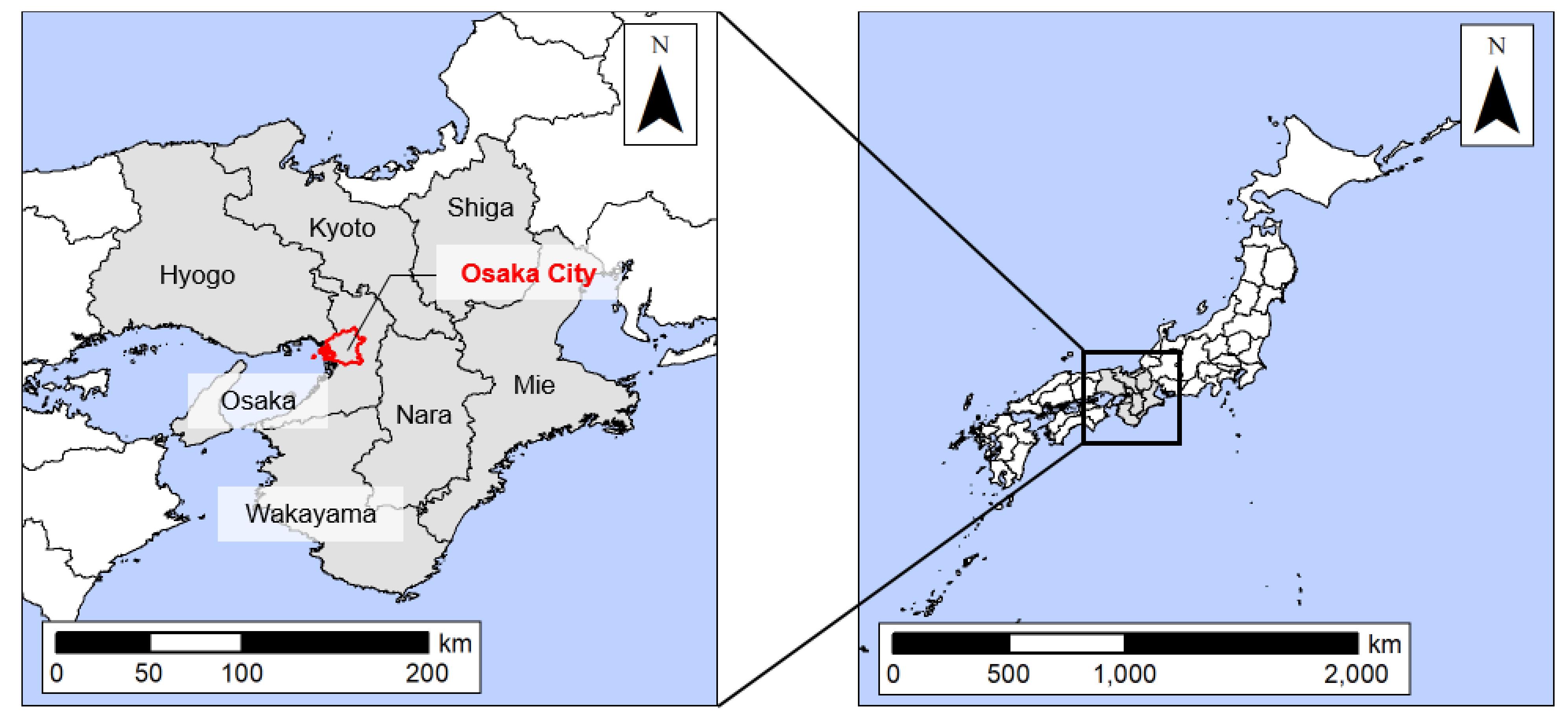
In this study, given that NO2 and VOC cause the formation of O3, Osaka City (Figure 1) was selected as the case study area, where many emission sources of such precursors exist [11,12,13,14,15]. The Hanshin Industrial Zone, one of the three major industrial zones (Keihin, Chukyo, and Hanshin Industrial Zone), extends along the coast of Osaka Prefecture. The Hanshin Industrial Zone is the second largest in terms of the shipment value of manufactured goods, after the Chukyo Industrial Zone, which is centered on the automobile industry [11]. The NOx emissions from smoke in Hyogo Prefecture, which is included in the Hanshin Industrial Zone, was the third largest after Yamaguchi and Hokkaido Prefectures in fiscal year (FY) 2018 [12], which indicates the presence of large stationary sources. The industrial zone is also a source of VOC, and VOC emissions in Osaka Prefecture in FY2018 was 31,789 t/year, the largest in western Japan [13]. In addition, Osaka Prefecture had the greatest transport ton-kilometers (12,705,503 thousand ton-kilometers) in FY2019 among the six major prefectures (Tokyo, Kanagawa, Aichi, Osaka, Hyogo, and Fukuoka Prefectures) [14] and the second greatest transport person-kilometers (5,160,352 thousand person-kilometers) in FY2019, following Tokyo Prefecture, the capital of Japan [15]; thus, mobile sources are also sufficient in the case study area.
Thus, although the existence of NOx emissions is sufficient for there to be a VOC-sensitive condition, the results of sensitivity regime diagnostics with satellite data show that the area around Osaka City has a mixed sensitivity, which is intermediate between NOx- and VOC-sensitive conditions [16], or there are two sensitive conditions (NOx- and VOC-sensitive ones) [17]. However, it has not been revealed which state is currently predominant in the city. Therefore, this study selected Osaka City, which has a large, exposed population and where the risk of increased O3 concentration caused by decreased NO2 concentration is unknown.
3. Methods
3.1. Estimation of Atmospheric Chemical Concentration and Measurement of Sensitive Conditions
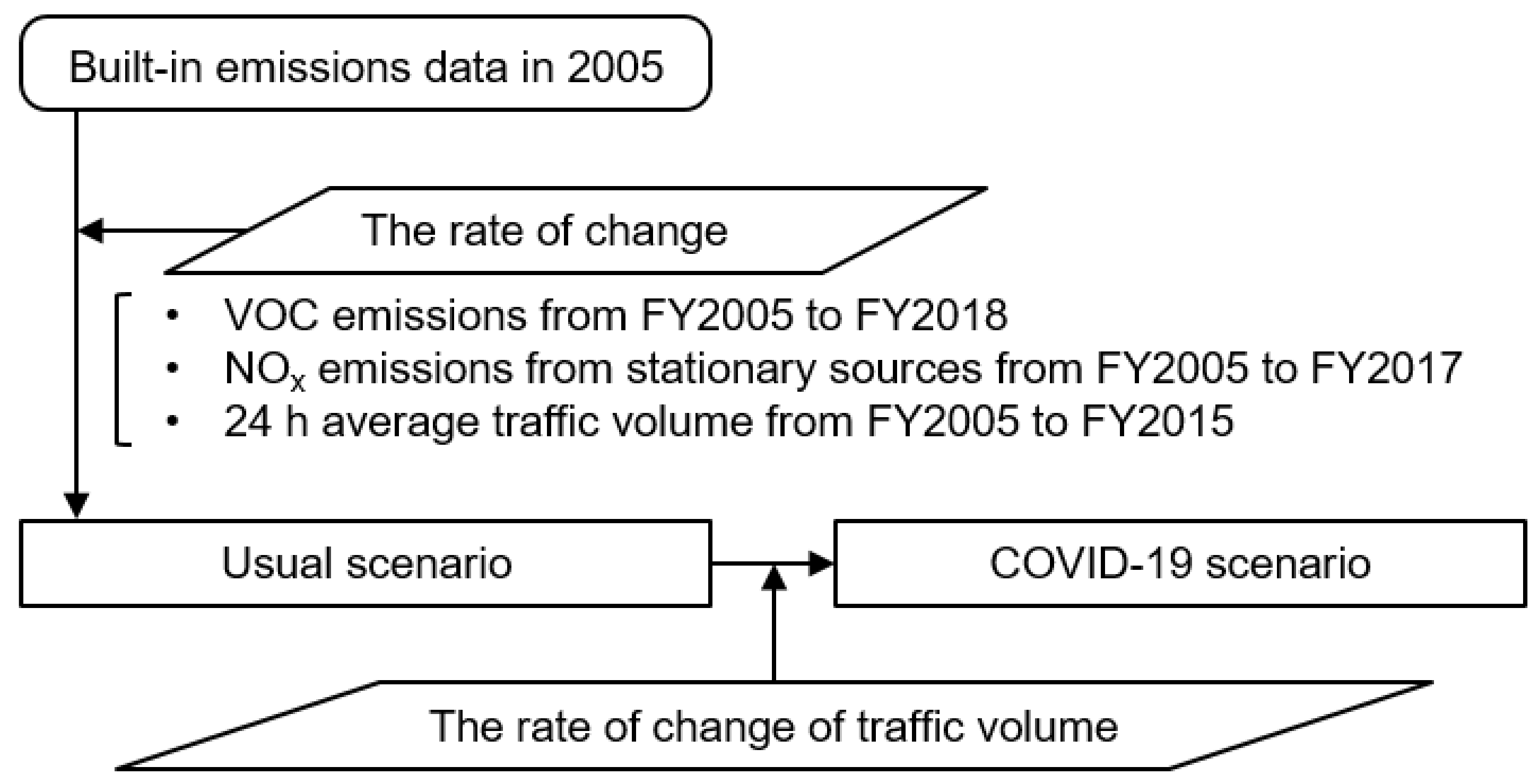
In this study, ADMER PRO Version 1.0 (ADMER-PRO) [18], which was developed by National Institute of Advanced Industrial Science and Technology (AIST) in Tsukuba, Japan, was used in estimating the concentrations of VOC, O3, and NOx, including NO and NO2. This is an atmospheric model for evaluating regional concentration distributions and can estimate the atmospheric concentration distributions of chemical substances, including secondary products, by using the chemical transport model [18]. ADMER-PRO includes emissions and meteorological data in 2005 (Figure 2). The meteorological data were processed from observed data by the National Centers for Environmental Prediction [19]. For stationary VOC sources, stationary NOx sources, and mobile NOx sources, we can simulate recent situations by comparing the actual emission data in 2005, which were included in the model, with the latest available emission data and by inputting the rate of change by prefecture. Given that NOx emissions from automobiles, which are mobile NOx sources, are not reported, the rate of the 24 h average traffic volume was substituted as the rate of NOx emissions. However, biogenic VOC (BVOC) emissions under standard meteorological conditions [20,21] were used and substantially revised significantly upward according to the results of field surveys and numerical experiments conducted by the AIST [22].
For stationary VOC sources, the VOC emission inventory data [13] were used in calculating the rate of change in VOC emissions from FY2005 to FY2018 by prefecture and industry (Figure 2). These data are published two years after Ministry of the Environment (MOE) estimates VOC emissions by industry for each fiscal year for the purpose of monitoring the progress of VOC emission control [13]. Here, we used the latest published VOC emissions in FY2018 [13]. For stationary NOx sources, a comprehensive survey on air pollutant emissions [12,23] was used in calculating the rate of change in NOx emissions from factories and power plants from FY2005 to FY2017 by prefecture (Figure 2). The survey is a statistical survey conducted every three years by the MOE for the monitoring of the emission status of air pollutants emitted from apparatus exhausting flue gas [12,23]. Here, we used the latest published NO2 emission data in FY2017 [12]. For mobile NOx sources, the Road Traffic Census [24,25] was used in calculating the rate of change in 24 h average traffic volume on weekdays from FY2005 to FY2015 by prefecture (Figure 2). This survey is a statistical survey conducted by Ministry of Land, Infrastructure, Transport and Tourism every five years [24,25]. Here, we used the latest published 24 h average traffic volume in FY2015 [25]. However, given that the traffic volume decreased by only 1.7% from FY2010 to FY2015 [26], we supposed that the data in FY2015 were sufficient to reproduce more recent situations. Using the emission data corrected by the above calculations, the average values from April to September (see Section 3.2 for the explanation on the selection of this period) of the concentrations of VOC and NOx and the sum of NO and NO2 were outputted using CB-IV 99, which is a built-in model that aggregates the formation of secondary pollutants, such as O3 and aldehydes, by grouping VOC into 37 chemical species and 93 chemical formulas based on their carbon bonding states [20]. In particular, given that the O3 concentration varies greatly with time, the daily maximum hourly value, which is related to health risk, was outputted using CB-IV 99.
VOC/NOx concentration ratio ([VOC]/[NOx]) [5,27,28] was used as an indicator to measure the sensitive conditions. When the value of this indicator is relatively small, the intensity of VOC-sensitivity is high, whereas when the value of this indicator is relatively large, the NOx-sensitive intensity is high [27]. Kannari [28] estimated that in the Kansai region, including Osaka Prefecture, the boundary value for the sensitive conditions is 6 to 12 for non-methane hydrocarbons (NMHC)/NOx concentration ratio. Since methane is not included in the VOC output by ADMER-PRO, we refer to its value as a boundary in this study.
3.2. Setting of Meteorological Conditions and Grids
The photochemical oxidant (OX) concentration increases during warmer seasons [29]. The total time when the hourly OX concentration in Osaka City exceeded the environmental quality standard of 60 ppb was highest from April to September [30]. Therefore, we set these months as the calculation period in this study. OX is a general term for oxidizing substances, excluding NO2, that can be measured using the neutral buffered potassium iodide method and include not only O3 but also peroxyacetylnitrate. In this study, OX and O3 concentrations were assumed to be equal, because O3 accounts for most of OX. ADMER-PRO is equipped with a “long-term analysis mode” that uses the classification of weather patterns to estimate the concentration over the target period in a relatively short time [22]. In the long-term analysis mode, the weather patterns of the target areas, which are grouped by weather pattern, are characterized on each day, and the appearance frequency of each weather pattern is calculated until the appearance frequency reaches a specified value [31]. In this study, the top five weather patterns with the highest appearance frequencies from April to September were used to shorten the calculation time, which includes three days of weather by each weather pattern. The AIST indicates that the coefficient of determination is 0.77 when the top five weather patterns are considered [22].
In addition, two grids were set up: one for the area to be analyzed and the other for the larger area covered with a rough resolution. For Osaka City, the target area, a 1 km × 1 km grid was set. For the larger area, a 5 km × 5 km grid was set for Kinki region (Mie, Shiga, Kyoto, Osaka, Hyogo, Nara, and Wakayama Prefectures), assuming that O3 and its precursors are transported from outside the target area [32].
3.3. Reduction of Traffic Volume during the COVID-19 Pandemic
In this study, we compared and analyzed two scenarios: a scenario reflecting the normal situation in recent years (usual scenario) and a scenario for reduced traffic due to the declaration of the state of emergency for COVID-19 (COVID-19 scenario), as shown in Figure 2 with the dataset and analysis procedure. The NOx emission sources include power plants and refuse incineration plants, which support the lives of citizens [33,34]; they were assumed to have been operating normally during the declaration of the state of emergency. To simulate the conditions based on the reduction of traffic volume due to COVID-19, at first, we extracted the rate of year-on-year change in traffic volume of major sections of expressways (West Nippon Expressway, Honshu-Shikoku Bridge Expressway, and Hanshin Expressway) in the Hanshin area only on weekdays and averaged over the period of declaration of the state of emergency [3]. Next, the rate of year-on-year change in traffic volume of general roads was calculated by extracting the rate of year-on-year change in traffic volume of National Route 1 on weekdays and averaged over the period of the declaration of the state of emergency [3]. The rate of year-on-year change of expressways and general roads was set uniformly in the Kinki region, including Osaka City. Finally, we multiplied the 24 h average traffic volume on expressways and general roads in FY2015 by the rate of year-on-year change in traffic volume for each road type and calculated the rate of change in traffic volume during the period of the declaration of the state of emergency, with weighting of the traffic volume for each road type by prefecture:
where Ri is the rate of change of traffic volume in the COVID-19 scenario, and a and b are the rates of year-on-year change in traffic volume for expressways and general roads, respectively. TEi and TGi are the usual traffic volumes for expressways and general roads, respectively.
The rate of year-on-year change in traffic volume in the Kinki region was 72.5% for expressways and 93.7% for general roads during the period of the declaration of the state of emergency [3]. Based on these values, we set the rate of change in traffic volume during the period of the declaration of the state of emergency as a = 0.7 and b = 0.9 and estimated that the rates were 0.72 in Nara Prefecture, 0.73 in Mie and Shiga Prefectures, and 0.74 in other prefectures (Kyoto, Osaka, Hyogo, and Wakayama Prefectures). These values were multiplied by the rate of change in mobile NOx sources by prefecture in the usual scenario and inputted into ADMER-PRO.
In this study, the annual change in health risk was estimated with the assumption that the reduction in traffic volume during the period of the declaration of state of emergency (7 April to 21 May 2020) would continue for one year. We used the reduction in traffic volume during the period of the declaration of the state of emergency to estimate the annual change in health risk because the impact of COVID-19 is still continuing, and the continuous reduction in traffic volume should be considered. In addition, the health risk is comparable with those of other diseases, which are generally estimated using the annual loss of disability-adjusted life years (DALY) as an indicator.
3.4. Validation of the Model
In this study, the reproducibility of the model was evaluated using the normalized mean bias (NMB), normalized mean error (NME), and the probability of factor 2 (Pfac2), which are widely used in the evaluation of atmospheric model performances [35,36]. The smaller the absolute value of NMB (Equation (4)) and the smaller the value of NME (Equation (5)), the higher the reproducibility [35].
where Calk is the estimated value, Obsk is the observed value, and N is the number of data. In this study, as substances for estimating health risks, the average NO2 concentrations estimated from April to September and the average O3 concentrations estimated at 14:00 of the specific weather patterns from April to September were compared with the average concentrations observed in FY2018 in the grid where each concentration was estimated. In Osaka City, NO2 and O3 concentrations were observed at 25 and 14 stations, respectively, in FY2018 [37].
3.5. Estimation of Health Risk Derived from O3
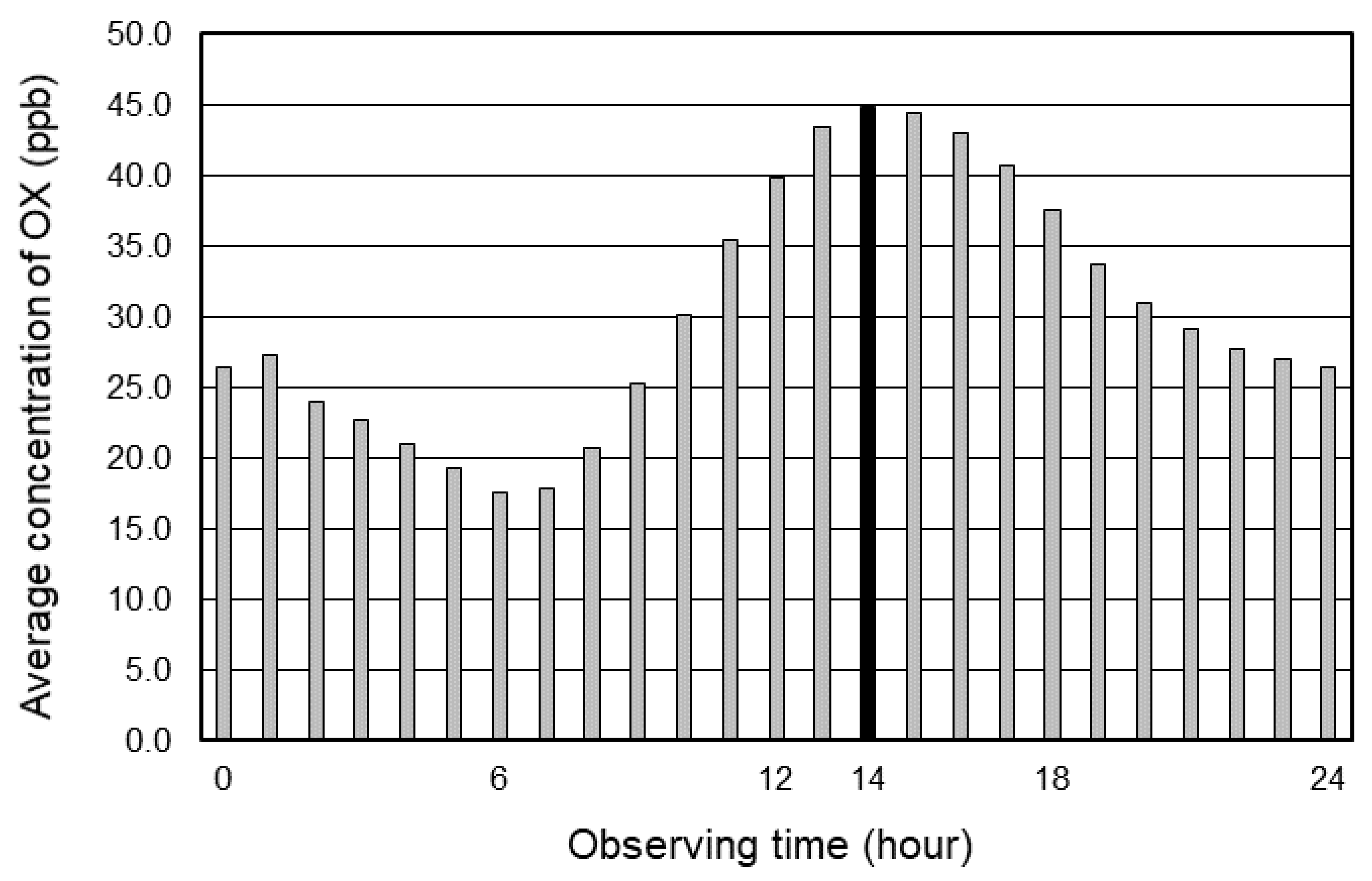
In this study, a 0.32% increase in mortality with a 10 ppb increase in the 24 h value of O3 concentration [8] was converted to a 0.17% increase in mortality, with the adoption of a 10 ppb increase in the daily maximum hourly value of O3 [38]. These values were based on the results of Bell et al. [8], who observed that the percentage increase in all-cause mortality associated with a 10 ppb increase in O3 concentration was 0.32% for a 1-day lag across the 98 U.S. communities. Nakanishi et al. [38] also adopted the value reported by Bell et al. [8], which was considered to have less uncertainty. On the other hand, a positive correlation exists between the daily maximum hourly value and the number of deaths due to respiratory disease [39]. Therefore, we calculated the average concentration at each hour from the observed values, excluding missing, unobserved, and error values, at 14 stations in Osaka City and used the estimated values for health risk assessment at 14:00 when the concentration was the highest [40] (Figure 3).
DALY, as an index of health risk, refers to the years lost due to death or disability, and it can comprehensively represent the burden of disease [41]. By evaluating health risk in terms of DALY, the health risk can potentially be compared with other diseases. DALY is the sum of years of life lost (YLL) and years lost due to disability [41]; however, given that the endpoint of this study increased mortality, only YLL was considered. YLL is calculated as the product of the number of deaths and life expectancy per age group [41]. The vital statistics [42] were used for the number of deaths and the life tables [43] for the life expectancy; the YLLs were calculated for each 5-year age group and finally summed to calculate the change in health risk:
where ∆DALY is the change in health risk, Casej is the number of deaths from causes other than injury disease at age j, RR is the relative risk of a 10 ppb increase in O3 concentration, and Lj is the life expectancy at age j. Based on the values of Bell et al. [8] and Nakanishi et al. [38], we calculated the health risk for usual and COVID-19 scenarios by using RR-1 of 0.0017. ∆C is the difference between the average O3 concentration estimated at 14:00 of the specific weather patterns from April to September averaged over Osaka City and the background concentration. We adopted the minimum concentration estimated for the usual scenario by ADMER-PRO as the background concentration [38].
3.6. Estimation of Health Risk Derived from NO2
Chen et al. [44] showed a 1.63% increase in daily mortality with a 10 μg/m3 increase in the 24 h value of NO2 concentration from the exposure–response relationship between NO2 concentration and daily deaths in 17 Chinese cities. In this study, the mass concentration of NO2 (a 1.63% increase with a 10 μg/m3 increase in the 24 h value) was converted to a volume concentration (a 3.08% increase with a 10 ppb increase in the 24 h value) at 23.8 °C, the observed temperatures in Osaka City from April to September in FY2018 was averaged [40]. However, the 0–4-year-old group was excluded from this study [44]. Based on the values, the health risks for usual and COVID-19 scenarios were evaluated in terms of DALY in Equation (6) and the estimation of health risk due to O3. Meanwhile, RR-1 was set at 0.0308; ∆C is the difference between the average NO2 concentrations estimated from April to September averaged over Osaka City and the minimum concentration estimated for usual scenarios by ADMER-PRO as the background concentration [38].
4. Results and Discussion
4.1. Validation of the Model
The average NO2 concentrations estimated from April to September by ADMER-PRO were compared with the average concentrations observed for the same period in FY2018 in the grid where the concentrations were estimated. The results were 0.315 for NMB and 0.339 for NME. These findings can be attributed to the difference in the distribution of emission sources from FY2005. Thus, certain emission sources existed in FY2005 that were absent in FY2018 due to environmental pollution control or population decrease, and the estimated values were overestimated compared with the observed values. However, Pfac2 was 100%, and all estimated values were contained within two times the observed value.
Similarly, for O3 concentrations, NMB and NME were both 0.301. The estimated values were higher than the observed ones at all stations, whereas Pfac2 was 100%. These differences between the estimated and measured values may have been caused by the difference in the distribution of emission sources and weather patterns of the observed values that were not included in the top five most frequently appearing weather patterns from April to September in this study. As a result, the mean of the observed values decreased. Based on these results, we considered this model to be sufficiently applicable for risk assessment, although it slightly overestimates the estimated values.
4.2. Estimation of Atmospheric Chemical Concentration and Measurement of Sensitive Conditions
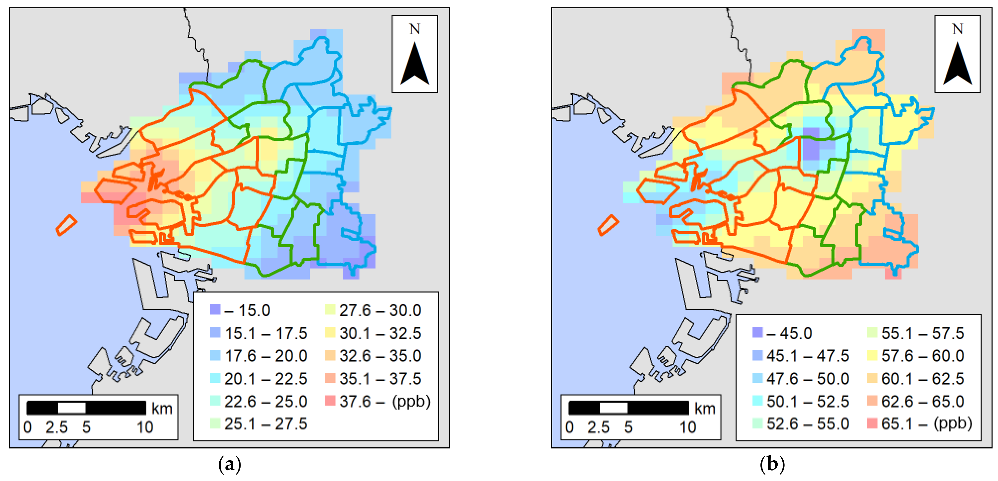
Figure 4 shows the average NO2 concentrations estimated from April to September and average O3 concentrations estimated at 14:00 of the specific weather patterns from April to September for the usual and COVID-19 scenarios. In both scenarios, NO2 concentrations were higher in coastal areas (Figure 4a), whereas O3 concentrations were lower in coastal and central areas, showing a distribution opposite to that of NO2 concentrations (Figure 4b). The low O3 concentrations, especially in the coastal areas, is attributed to the reaction of NO2, which also showed high concentrations in these areas, with OH interfering with the chain reaction cycle from (R4,5) to (R1), (R2), which starts from the reaction of OH with VOC, resulting in a decrease in O3 production efficiency.
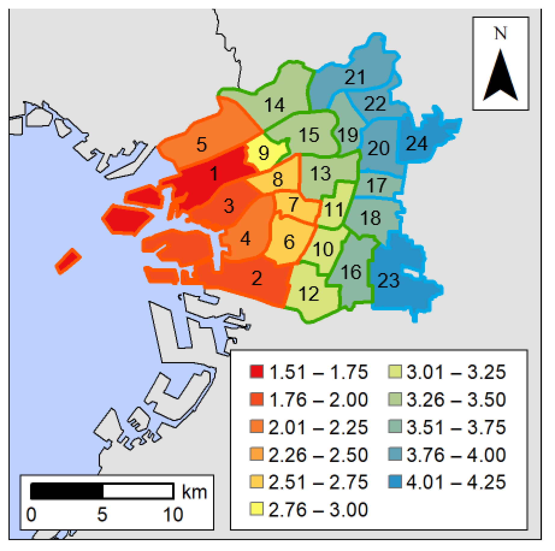
Table 1 lists the VOC/NOx concentration ratios (in ascending order) obtained from the average VOC and NOx concentrations estimated from April to September for each ward, and Figure 5 shows the VOC/NOx concentration ratio with the location of each ward. Since the VOC/NOx concentration ratios of all the wards were below 6 to 12, as indicated by Kannari [28], overall, Osaka City had a high intensity of VOC-sensitivity. Therefore, we divided the ward into three groups of eight wards, starting from the ward with the smallest concentration ratio and the highest intensity of VOC-sensitivity, and classified them based on high (Group High), middle (Group Middle), and low (Group Low) intensities of VOC-sensitivity (Figure 5). The average VOC concentrations in each group were 71.4, 85.7, and 90.7 ppb, and the average NOx concentrations were 33.8, 26.8, and 23.7 ppb. Group High mainly included coastal areas, and Group Middle to Group Low comprised inland wards. The top ten wards with the highest VOC concentrations were distributed among the three groups, whereas seven of them with NOx concentrations were included in Group High. This finding indicates that NOx concentration contributed significantly to the group to which a ward belonged.
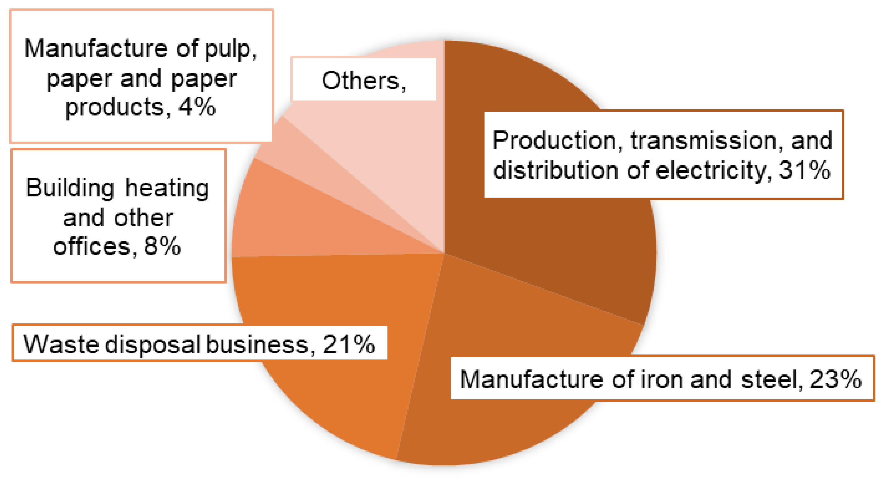
Two types of NOx emission sources exist: stationary sources, such as factories and power plants, and mobile sources, such as automobiles [33,34]. With regard to stationary NOx emission sources, Figure 6 shows the breakdown of NOx emissions in Osaka City in FY2018 by industry [12]. The production, transmission, and distribution of electricity accounted for the largest share at 31%, followed by the manufacture of iron and steel at 23%, waste disposal businesses at 21%, building heating and other offices at 8%, and the manufacture of pulp, paper, and paper products at 4% [12]. Konohana Ward (No. 1 in Figure 5), which has the smallest VOC/NOx concentration ratio in Osaka City and was included in Group High, has a refuse incineration plant (Maishima Plant) and a sewage sludge treatment plant (Maishima Sludge Center). In addition, Suminoe Ward (No. 2 in Figure 5), which had the next smallest VOC/NOx concentration ratio, has the only natural gas-fired power plant (Nanko Power Plant) in Osaka City, from which 165 t of NOx, corresponding to 6% of annual NOx emissions in Osaka City, were emitted in FY2018 [45]. These large-scale emissions of NOx are thought to have resulted in high NOx concentrations in the wards with the smallest VOC/NOx concentration ratios. In addition, Taisho Ward (No. 4 in Figure 5), which was included in Group High, had the largest, at 190,610 million yen, value of manufactured goods shipments of iron and steel in Osaka City in 2019 [46]; the other wards in Group High are also engaged in the industry (Table 1). By contrast, most of the wards in Group Middle and Group Low have no engagement in the industry (Table 1).
With regard to mobile NOx emission sources, Table 1 shows the total value of the product of section extension and 24 h traffic volume for each ward in FY2015 [25]. Six of the top ten wards were included in Group High. These results indicate that wards with high NOx concentrations had high emissions from stationary and mobile sources of NOx, which contributed to the VOC-sensitive condition.
4.3. Comparison of NO2 and O3 Concentrations Between Scenarios
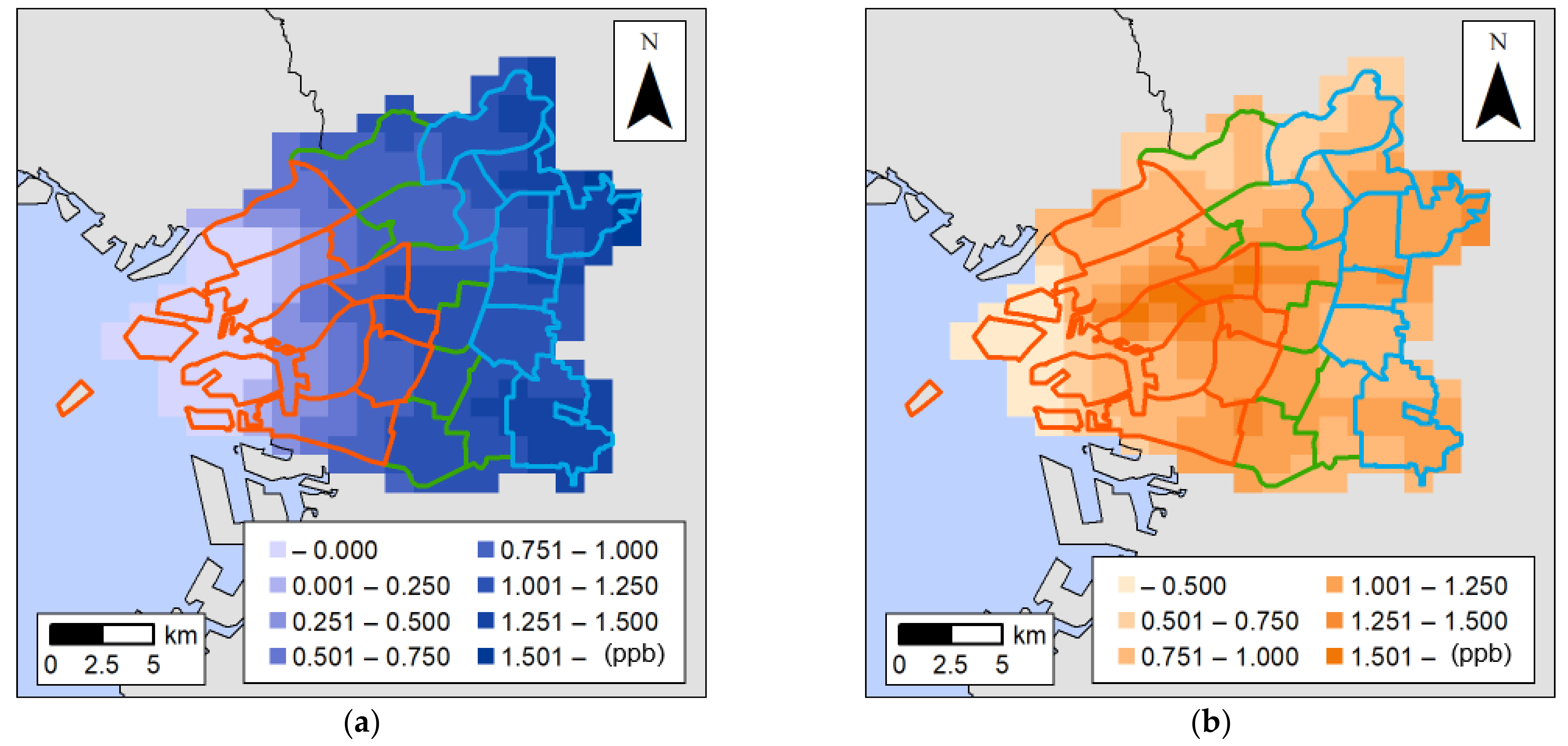
In the COVID-19 scenario, NO2 concentrations decreased by an average of 0.962 ppb in 88.9% of the grids in Osaka City compared with the usual scenario due to the reduction in traffic caused by COVID-19 (Figure 7a). Regarding the characteristics of each group, seven out of eight wards belonging to Group Low were among the top ten wards with the largest decrease in NO2 concentration (Table 2). On the other hand, Group High did not include any of these wards (Table 2) given the absence of significant stationary emission sources in Group Low (Table 1). Thus, the proportion of emissions from mobile sources was large, and the decrease in traffic volume in the COVID-19 scenario may have caused a large decrease in NO2 concentration in the wards belonging to Group Low. By contrast, Group High included significant stationary emissions, such as the power plant and refuse incineration plant. However, given that these operations continued in the COVID-19 scenario, the overall decrease in NO2 concentration was considered to be relatively small, although only the emissions from mobile sources decreased with the decrease in traffic. The NO2 concentration in Konohana Ward was 33.1 ppb in the usual scenario and 33.4 ppb in the COVID-19 scenario, resulting in an increase of 0.261 ppb. However, considering the possibility of overestimation using the NME in Section 4.1, the NO2 concentration was at its lowest at 22.1 ppb in the COVID-19 scenario. With the increase in 0.261 ppb being within the margin of error, it is unclear as to whether only NO2 the concentration in Konohana Ward followed an increasing trend.
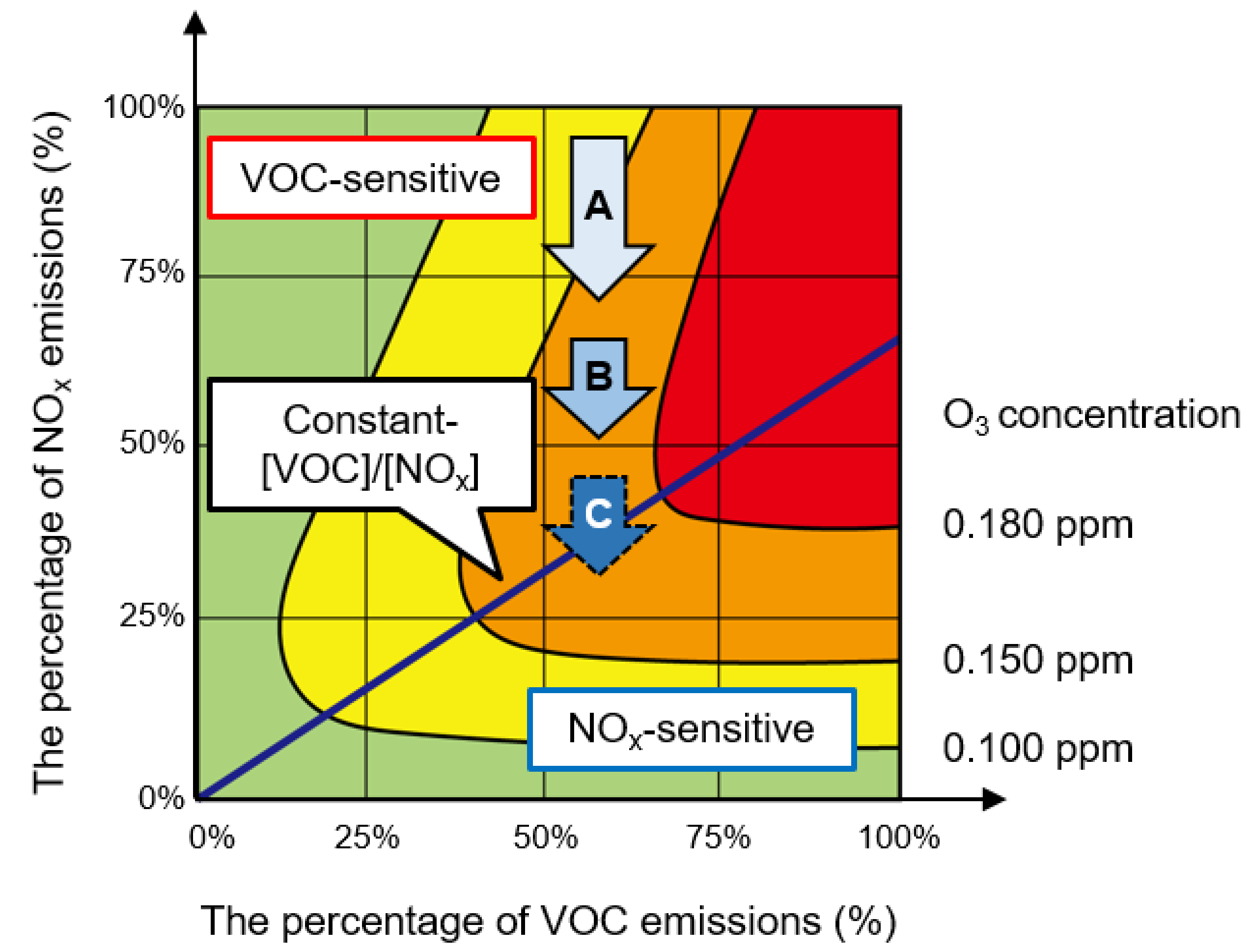
On the other hand, O3 concentrations in the COVID-19 scenario increased by an average of 1.00 ppb in all grids compared with the usual scenario (Figure 7b). The top 12 wards with the highest intensity of VOC-sensitivity included the top 10 wards with the largest increase in O3 concentration. In particular, Nishi (No. 8 in Figure 5), Naniwa (No. 7 in Figure 5), and Minato Wards (No. 3 in Figure 5), which belonged to Group High, had large increases of 1.39, 1.35, and 1.28 ppb, respectively. By contrast, one ward in Group Low, with the top 10 wards, showed the largest increase in O3 concentration. The wards in the former group were considered to be in phase A in Figure 8, where O3 concentration increased in the VOC-sensitive condition. If the reduction of NO2 emissions continues, the O3 concentration is expected to remain almost constant as the amount of NO2 supplied to (R1) decreases, while the amount of NO2 produced in (R4) will increase due to the acceleration of the chain reaction cycle. However, given the continuity of VOC-sensitive conditions, the O3 concentration may increase further if VOC emissions increase in this condition. By contrast, the wards in the latter group were considered to be in phase B in Figure 8, given the small increase in O3 concentration. If the decrease in NO2 emissions continues further, the condition will shift to the NOx-sensitive condition in phase C in Figure 8. In such a case, the O3 concentration is expected to decrease further with the decrease in NO2 emissions, and the O3 concentration is expected to remain constant when the VOC concentration increases.
4.4. Health Risk Derived from NO2 and O3
Table 3 shows the health risks from NO2 and O3 for the usual and COVID-19 scenarios, and the increase/decrease in health risk from the usual scenario to the COVID-19 scenario. For the usual scenario, the health risks of NO2 and O3 for the whole of Osaka City were 9454 and 1310 DALYs, respectively. In the COVID-19 scenario, the health risk from NO2 was 811.4 DALYs (8.6%) lower, at 8643 DALYs, whereas that from O3 was 55.90 DALYs (4.3%) higher, at 1365 DALYs. Given that Chen et al. [44] only showed mortality rates for the combination of NO2, particulate matter (PM10), and sulfur dioxide, the endpoint in this study was the increase in mortality when only the relevant substances increased (single-pollutant model), in order to reduce uncertainty. Therefore, considering these health risks simultaneously is difficult. However, decreased NOx emissions will increase the O3 concentration and the health risk from O3, but will substantially decrease the health risk from NO2. This condition is due to the greater loss in health risk per concentration of NO2 (RR-1 = 0.0308) compared with that of O3 (RR-1 = 0.0017), although the change in O3 concentration was larger than that in the NO2 concentration in Osaka City. In this study, we estimated the health risk for the whole of Osaka City. The daytime population of Nishi, Naniwa, Minato, and Nishinari Wards (No. 6 in Figure 5) in Group High and Chuo Ward (No. 13 in Figure 5) in Group Middle, where the increase in O3 concentration, was large, and exceeded the night-time population; the daytime population of Chuo Ward is about five times larger than the night-time population [48]. Therefore, the health risk in these wards may be high, because the population coming in from outside the ward during daytime may be exposed to increased O3.
When we used the NME to calculate the health risks from O3 and NO2 by correcting for the overestimated values of the two scenarios, the decrease in health risk from NO2 was 14.5 times greater than the increase in health risk from O3 before the correction and 13.7 times greater after the correction. This result indicates that errors in the model caused no effects on the results obtained in this study. On the other hand, given that we estimated DALYs per year using O3 concentration estimated for a specific weather pattern from April to September in this study, the DALYs were possibly overestimated, considering that O3 concentrations decrease in winter. However we concluded that this overestimation is acceptable.
5. Conclusions
In this study, we quantitatively clarified that Osaka City was in a VOC-sensitive condition, where the sensitive condition has not been clearly measured. The study also demonstrated that different sensitive conditions can occur because of differences in the distributions of NOx emission sources and emissions, even in narrow areas of the same city. Moreover, the results of the study enabled us to predict O3 concentration variations due to reductions in NO2 emissions and to quantitatively evaluate associated health risks with DALY that were previously unknown. The risk assessment method and the results obtained through ADMER-PRO and DALY produced valuable findings for determining future policies on air pollution control.
The VOC/NOx concentration ratio was calculated for each ward, and the results showed that the intensity of VOC-sensitivity was higher in coastal areas and lower toward inland areas. In Group High, with a high intensity of VOC-sensitivity, large-scale emissions of NOx, such as those from a power plant, a refuse incineration plant, a sewage sludge treatment plant, and a manufacturer of iron and steel, were located nearby, contributing to the VOC-sensitive condition. The top 12 wards with the highest intensities of VOC-sensitivity exhibited large increases in O3 concentrations, with a 26–28% reduction in NOx emissions from mobile sources in the Kinki region. However, it is unlikely that O3 concentrations will increase rapidly in the future, despite the further reduction in NO2 emissions. Still, if NO2 decreases in these areas, the VOC-sensitive condition is expected to continue for a time, and O3 concentrations may increase further as VOC concentrations increase, which may increase the health risk from O3. Furthermore, given that the daytime population exceeds the night-time population in coastal and central areas where the increase in O3 concentration was large, the health risk in those wards may be greater. On the other hand, Group Low showed a large reduction in NO2 concentrations in the COVID-19 scenario because of the relatively large amount of emissions from mobile sources. In addition, the increase in O3 concentration was relatively small in the wards belonging to this group, suggesting that the continuous decrease in NO2 emissions in the future may shift to the NOx-sensitive condition and trigger a decrease in O3 concentration.
As a result of traffic reduction, the health risk from NO2 decreased by 811.4 DALYs, and that from O3 increased by 55.90 DALYs, for the entirety of Osaka City.
This study showed that in Osaka City, which is a VOC-sensitive area, the decrease in health risk due to the reduction in NOx emissions from mobile sources exceeds the increase in health risk due to the increased O3 concentration, regardless of the sensitive conditions, indicating that the reduction in NO2 emissions reduces the net health risk from air pollutants. Therefore, the health risk is expected to decrease even under (i) a lockdown due to further spread of COVID-19, (ii) a decrease in traffic volume due to road damage caused by large-scale natural disasters, or (iii) a decrease in NOx emissions due to alternative means of transportation, such as the widespread use of next-generation vehicles. In addition, given the regional variation of vegetation, which are the major source of VOC emissions, the health risk from NO2 and O3 in other regions can be estimated, provided that the appropriate amount of BVOC emissions is set.
Author Contributions
Conceptualization, Y.O., L.I. and A.T.; methodology, Y.O. and L.I.; validation, Y.O., L.I. and A.T.; formal analysis, Y.O.; investigation, Y.O. and L.I.; data curation, Y.O.; writing—original draft preparation, Y.O.; writing—review and editing, L.I. and A.T.; visualization, Y.O.; supervision, L.I. and A.T.; project administration, A.T.; funding acquisition, A.T. All authors have read and agreed to the published version of the manuscript.
Funding
This research was funded by Study on Sound Management of Chemicals with Relevant Legal Framework (METI) in FY2020 and the Environment Research and Technology Development Fund (JPMEERF18S11702) of the Environmental Restoration and Conservation Agency of Japan.
Institutional Review Board Statement
Not applicable.
Informed Consent Statement
Not applicable.
Data Availability Statement
The data presented in this study are available upon request from the corresponding author.
Conflicts of Interest
The authors declare no conflict of interest.
References
- Velavan, T.P.; Meyer, C.G. The COVID-19 epidemic. Trop. Med. Int. Health 2020, 25, 278–280. [Google Scholar] [CrossRef] [PubMed] [Green Version]
- Gossling, S.; Scott, D.; Hall, C.M. Pandemics, tourism and global change: A rapid assessment of COVID-19. J. Sustain. Tour. 2020, 29, 1–20. [Google Scholar] [CrossRef]
- Changes in Traffic Volume on Major Sections of Expressways and Major National Highways in Major Urban Areas in Japan. Translated from Japanese. Available online: https://www.mlit.go.jp/road/road_fr4_000090.html (accessed on 1 February 2021).
- NASA Model Reveals How Much COVID-Related Pollution Levels Deviated from the Norm. Available online: https://www.nasa.gov/feature/goddard/2020/nasa-model-reveals-how-much-covid-related-pollution-levels-deviated-from-the-norm (accessed on 1 February 2021).
- Siciliano, B.; Dantas, G.; da Silva, C.M.; Arbilla, G. Increased ozone levels during the COVID-19 lockdown: Analysis for the city of Rio de Janeiro, Brazil. Sci. Total Environ. 2020, 737, 139765. [Google Scholar] [CrossRef] [PubMed]
- Hashim, B.M.; Al-Naseri, S.K.; Al-Maliki, A.; Al-Ansari, N. Impact of COVID-19 lockdown on NO2, O3, PM2.5 and PM10 concentrations and assessing air quality changes in Baghdad, Iraq. Sci. Total Environ. 2020, 754, 141978. [Google Scholar] [CrossRef] [PubMed]
- Peralta, O.; Ortinez-Alvarez, A.; Torres-Jardon, R.; Suarez-Lastra, M.; Castro, T.; Ruiz-Suarez, L.G. Ozone over Mexico City during the COVID-19 pandemic. Sci. Total Environ. 2020, 76, 143183. [Google Scholar] [CrossRef] [PubMed]
- Bell, M.L.; Peng, R.D.; Dominici, F. The exposure-response curve for ozone and risk of mortality and the adequacy of current ozone regulations. Environ. Health Perspect. 2006, 114, 532–536. [Google Scholar] [CrossRef] [PubMed] [Green Version]
- Jacob, D.J. Introduction to Atmospheric Chemistry; Princeton University Press: Princeton, NJ, USA, 1999. [Google Scholar]
- Survey on Scientific Knowledge on Photochemical Oxidants and Other Factors Related to the Atmospheric Environment (Summary). Translated from Japanese. Available online: https://www.meti.go.jp/shingikai/sankoshin/sangyo_gijutsu/sangyo_kankyo/pdf/006_02_02.pdf (accessed on 1 February 2021).
- Yanotsuneta Kinenkai. Japan National Census 2018/19; Translated from Japanese; Yanotsuneta Kinenkai: Tokyo, Japan, 2018. [Google Scholar]
- Comprehensive Survey on Air Pollutant Emissions (FY2017). Translated from Japanese. Available online: http://www.env.go.jp/air/air/osen/kotei/h30_2.pdf (accessed on 1 February 2021).
- FY2019 Volatile Organic Compounds (VOC) Emission Inventory Data. Translated from Japanese. Available online: https://www.env.go.jp/air/air/osen/voc/inventory/R1/R1-Mat02.xlsx (accessed on 1 February 2021).
- FY2019 Survey on Motor Vehicle Transport for Freight. Translated from Japanese. Available online: https://www.e-stat.go.jp/stat-search/files?page=1&layout=datalist&toukei=00600330&bunya_l=10&tstat=000001078083&cycle=8&year=20191&month=0&stat_infid=000031974557&result_back=1&result_page=1&tclass1val=0 (accessed on 1 February 2021).
- FY2019 Survey on Motor Vehicle Transport for Passenger. Translated from Japanese. Available online: https://www.e-stat.go.jp/stat-search/files?page=1&layout=datalist&toukei=00600330&bunya_l=10&tstat=000001078083&cycle=8&year=20191&month=0&stat_infid=000031974566&result_back=1&result_page=1&tclass1val=0 (accessed on 1 February 2021).
- Survey on Quantitative Evaluation of VOC Emission Reduction Effect. Translated from Japanese. Available online: https://www.meti.go.jp/shingikai/sankoshin/sangyo_gijutsu/sangyo_kankyo/pdf/008_02_02.pdf (accessed on 1 February 2021).
- Yamamoto, K. Consideration on photochemical oxidant production regime in Osaka. Bull. Res. Inst. Environ. Agric. Fish. Osaka Prefect. 2014, 1, 9–14. [Google Scholar] [CrossRef]
- ADMER-PRO Ver.1.0 (Atmospheric Dispersion Model for Exposure and Risk Assessment). Available online: https://admer-pro.aist-riss.jp/ (accessed on 1 February 2021).
- Operating Manual for ADMER PRO Version 1.0. Translated from Japanese. Available online: https://admer-pro.aist-riss.jp/wp-content/uploads/sites/92/2015/08/ADMER-PRO_V10_manual.pdf (accessed on 1 February 2021).
- Inoue, K.; Yasuda, R.; Yoshikado, H.; Higashino, H. Spatial distribution of summer-time surface ozone sensitivity to NOx and VOC emissions for the Kanto area, part 1: Estimation by numerical simulations with two kinds of (larger and smaller) biogenic emission estimates. J. Jpn. Soc. Atmos. Environ. 2010, 45, 183–194. [Google Scholar] [CrossRef]
- Inoue, K.; Yoshikado, H.; Higashino, H. Spatial distribution of summer-time surface ozone sensitivity to NOx and VOC emissions for the Kanto area, part 2: Estimation based on the measurement of a photochemical indicator. J. Jpn. Soc. Atmos. Environ. 2010, 45, 195–204. [Google Scholar] [CrossRef]
- Technical Manual for ADMER-PRO Version 0.8β. Translated from Japanese. Available online: https://admer-pro.aist-riss.jp/wp-content/uploads/sites/92/2015/08/ADMER-PRO_V08B_techdisc.pdf (accessed on 1 February 2021).
- Comprehensive Survey on Air Pollutant Emissions (FY2005). Translated from Japanese. Available online: http://www.env.go.jp/air/osen/kotei/haishutsu/h18.pdf (accessed on 1 February 2021).
- Japan Society of Traffic Engineers (JSTE). FY2005 Road Traffic Census; Translated from Japanese; Maruzen Publishing: Tokyo, Japan, 2007. [Google Scholar]
- Japan Society of Traffic Engineers (JSTE). FY2015 Road Traffic Census; Translated from Japanese; Maruzen Publishing: Tokyo, Japan, 2018. [Google Scholar]
- Japan Society of Traffic Engineers (JSTE). FY2010 Road Traffic Census; Translated from Japanese; Maruzen Publishing: Tokyo, Japan, 2012. [Google Scholar]
- Yang, Y.; Liu, X.; Zheng, J.; Tan, Q.; Feng, M.; Qu, Y.; An, J.; Cheng, N. Characteristics of one-year observation of VOCs, NOx, and O3 at an urban site in Wuhan, China. J. Environ. Sci. 2019, 79, 297–310. [Google Scholar] [CrossRef] [PubMed]
- Kannari, A. An analysis of weekend effects on photochemical oxidant concentrations in the Kanto and Kansai regions Part 2 Verification of dynamically changing ozone formation regimes. J. Jpn. Soc. Atmos. Environ. 2006, 41, 220–233. [Google Scholar] [CrossRef]
- Monks, P.S. A review of the observations and origins of the spring ozone maximum. Atmos. Environ. 2000, 34, 3545–3561. [Google Scholar] [CrossRef]
- FY 2018 Air Environment Monthly and Annual Value Data. Translated from Japanese. Available online: https://www.nies.go.jp/igreen/td_down.html (accessed on 1 February 2021).
- Yoshikado, H.; Shirakawa, Y.; Nakano, T.; Kudo, Y.; Suzuki, M. Feasibility of a method simulating long-term average concentration of pollutants based on a mesoscale meteorological model (I) Classification of weather patterns and application to NOx in the Kanto Plain. J. Jpn. Soc. Atmos. Environ. 2006, 41, 1–14. [Google Scholar] [CrossRef]
- Chan, C.Y.; Chan, L.Y. Effect of meteorology and air pollutant transport on ozone episodes at a subtropical coastal Asian city, Hong Kong. J. Geophys. Res. 2000, 105, 20707–20724. [Google Scholar] [CrossRef] [Green Version]
- Nazari, S.; Shahhoseini, O.; Sohrabi-Kashani, A.; Davari, S.; Paydar, R.; Delavar-Moghadam, Z. Experimental determination and analysis of CO2, SO2 and NOx emission factors in Iran’s thermal power plants. Energy 2010, 35, 2992–2998. [Google Scholar] [CrossRef]
- Carslaw, D.C. Evidence of an increasing NO2/NOx emissions ratio from road traffic emissions. Atmos. Environ. 2005, 39, 4793–4802. [Google Scholar] [CrossRef]
- Inoue, K.; Higashino, H. Development and verification of the atmospheric model ADMER-PRO Applicable for Secondary Formation. J. Jpn. Soc. Atmos. Environ. 2015, 50, 278–291. [Google Scholar] [CrossRef]
- Itahashi, S.; Yamaji, K.; Chatani, S.; Kitayama, K.; Morino, Y.; Nagashima, T.; Saito, M.; Takigawa, M.; Morikawa, T.; Kanda, I.; et al. Model performance differences in fine-mode nitrate aerosol during wintertime over Japan in the J-STREAM model inter-comparison study. Atmosphere 2020, 11, 511. [Google Scholar] [CrossRef]
- FY2018 Results of Air Pollution Monitoring. Translated from Japanese. Available online: http://taiki.kankyo.pref.osaka.jp/taikikanshi/taiki_sokutei/H30_2018/taiki_h30(2018)_index.html (accessed on 1 February 2021).
- Nakanishi, J.; Shinozaki, H.; Inoue, K. Risk Assessment Documents for Ozone (Photochemical Oxidant); Translated from Japanese; Maruzen Pabulishing: Tokyo, Japan, 2009. [Google Scholar]
- Jerret, M.; Burnett, R.T.; Pope, C.A., III; Ito, K.; Thurston, G.; Kreski, D.; Shi, Y.; Calle, E.; Thun, M. Long-term ozone exposure and mortality. N. Engl. J. Med. 2009, 360, 1085–1095. [Google Scholar] [CrossRef] [PubMed] [Green Version]
- FY2018 Air Environment Hourly Value Data. Translated from Japanese. Available online: https://www.nies.go.jp/igreen/tj_down.html (accessed on 1 February 2021).
- Murray, C.J.L.; Lopez, A.D. The Global Burden of Disease; Harvard School of Public Health: Boston, MA, USA, 1996. [Google Scholar]
- 2018 Vital Statistics. Translated from Japanese. Available online: https://www.e-stat.go.jp/stat-search/files?page=1&layout=datalist&toukei=00450011&bunya_l=02&tstat=000001028897&cycle=7&year=20180&month=0&tclass1=000001053058&tclass2=000001053061&tclass3=000001053074&tclass4=000001053089&stat_infid=000031884414&result_back=1&result_page=1&tclass5val=0 (accessed on 1 February 2021).
- 2015 Life Tables. Translated from Japanese. Available online: https://www.e-stat.go.jp/stat-search/files?page=1&layout=datalist&toukei=00450012&bunya_l=02&tstat=000001031336&cycle=7&tclass1=000001060926&tclass2=000001114595&stat_infid=000031693271&tclass3val=0 (accessed on 1 February 2021).
- Chen, R.; Samoli, E.; Wong, C.M.; Huang, W.; Wang, Z.; Chen, B.; Kan, H. Associations between short-term exposure to nitrogen dioxide and mortality in 17 Chinese cities: The China Air Pollution and Health Effects Study (CAPES). Environ. Int. 2012, 45, 32–38. [Google Scholar] [CrossRef] [PubMed]
- Environmental Data 2019. Translated from Japanese. Available online: https://www.kepco.co.jp/sustainability/kankyou/report/pdf/k_report2019.pdf (accessed on 1 February 2021).
- 2019 Census of Manufacture. Translated from Japanese. Available online: https://www.e-stat.go.jp/stat-search/files?page=1&layout=datalist&toukei=00550010&tstat=000001022686&cycle=7&tclass1=000001022790&tclass2=000001143706&stat_infid=000031975100&tclass3val=0 (accessed on 1 February 2021).
- Report of the Study Group on Photochemical Oxidants. Translated from Japanese. Available online: https://www.env.go.jp/air/osen/pc_oxidant/conf/chosa.html (accessed on 1 February 2021).
- 2015 National Census. Translated from Japanese. Available online: https://www.e-stat.go.jp/stat-search/files?page=1&layout=datalist&toukei=00200521&bunya_l=02&tstat=000001080615&cycle=0&tclass1=000001101935&tclass2=000001101955&tclass3=000001101982&stat_infid=000031587080&result_page=1&tclass4val=0 (accessed on 1 February 2021).
Figure 1.
Location of Osaka City. Osaka City is the prefectural capital of Osaka Prefecture and consists of 24 wards. The gray area covers the Kinki region, which consists of Mie, Shiga, Kyoto, Osaka, Hyogo, Nara, and Wakayama Prefectures.
Figure 1.
Location of Osaka City. Osaka City is the prefectural capital of Osaka Prefecture and consists of 24 wards. The gray area covers the Kinki region, which consists of Mie, Shiga, Kyoto, Osaka, Hyogo, Nara, and Wakayama Prefectures.

Figure 2.
Analysis procedure. Rounded rectangle represents initial data, parallelograms represent input data, rectangles represent scenarios, and arrows represent analysis procedures.
Figure 2.
Analysis procedure. Rounded rectangle represents initial data, parallelograms represent input data, rectangles represent scenarios, and arrows represent analysis procedures.

Figure 3.
Hourly average concentration of OX observed at 14 stations in Osaka City from April to September in 2018 [40]. The concentration at 14:00 was the highest, at 44.9 ppb.
Figure 3.
Hourly average concentration of OX observed at 14 stations in Osaka City from April to September in 2018 [40]. The concentration at 14:00 was the highest, at 44.9 ppb.

Figure 4.
NO2 and O3 concentrations in the usual scenario estimated by ADMER-PRO. (a) Average NO2 concentrations estimated from April to September and (b) average O3 concentrations at 14:00 of the specific weather patterns from April to September. The red, green, and blue boxes correspond to Group High, Group Middle, and Group Low, respectively.

Figure 5.
VOC/NOx concentration ratios for each ward. Numbers were assigned to each ward, from the smallest concentration ratio, namely, the highest intensity of VOC-sensitivity. The red, green, and blue boxes correspond to Group High, Group Middle, and Group Low, respectively.
Figure 5.
VOC/NOx concentration ratios for each ward. Numbers were assigned to each ward, from the smallest concentration ratio, namely, the highest intensity of VOC-sensitivity. The red, green, and blue boxes correspond to Group High, Group Middle, and Group Low, respectively.

Figure 6.
Breakdown of NO2 emissions from the industrial sector in Osaka City in FY2018 [12]. A total of 2699 t/year of NO2 was emitted from all sectors in Osaka City in FY2018.
Figure 6.
Breakdown of NO2 emissions from the industrial sector in Osaka City in FY2018 [12]. A total of 2699 t/year of NO2 was emitted from all sectors in Osaka City in FY2018.

Figure 7.
Differences in concentrations between the usual and COVID-19 scenarios. (a) Average NO2 concentration estimated from April to September in the usual scenario minus the value in the COVID-19 scenario; and (b) average O3 concentration estimated at 14:00 for the specific weather patterns from April to September in the COVID-19 scenario minus the value in the usual scenario. The red, green, and blue boxes correspond to Group High, Group Middle, and Group Low, respectively.

Figure 8.
Dependence of O3 concentration on VOC and NOx emissions and isoconcentration area of O3. The vertical and horizontal axes represent the percentage of NOx and VOC emissions, respectively. The center line represents the border of NOx- and VOC-sensitive conditions, above which is the VOC-sensitive condition, and below which is the NOx-sensitive one. The same color area represents the same O3 concentration. (Modified from the MOE [47]).


Table 1.
VOC/NOx concentration ratio, VOC and NOx concentrations by ward, the value of manufactured goods shipments of iron and steel [46], and product of section extension and 24 h traffic volume for each ward [25].
| No. | Ward | Group | [VOC]/[NOx] | [VOC] (ppb) | [NOx] (ppb) | Shipment Value of Iron and Steel Industry (Million Yen) | Product of Traffic Volume and Section Extension (thousand car-km/day) |
|---|---|---|---|---|---|---|---|
| 1 | Konohana | High | 1.51 | 62.8 | 41.7 | 55,836 | 599 |
| 2 | Suminoe | 1.77 | 61.8 | 34.9 | 43,363 | 1101 | |
| 3 | Minato | 1.81 | 69.1 | 38.1 | 1407 | 765 | |
| 4 | Taisho | 2.12 | 68.5 | 32.4 | 190,610 | 284 | |
| 5 | Nishiyodogawa | 2.23 | 69.1 | 30.9 | 112,308 | 1020 | |
| 6 | Nishinari | 2.55 | 71.6 | 28.1 | 7012 | 694 | |
| 7 | Naniwa | 2.58 | 78.7 | 30.5 | 3026 | 678 | |
| 8 | Nishi | 2.65 | 89.9 | 34.0 | 3126 | 1033 | |
| 9 | Fukushima | Middle | 2.78 | 84.2 | 30.2 | - | 584 |
| 10 | Abeno | 3.02 | 74.1 | 24.5 | - | 485 | |
| 11 | Tennoji | 3.08 | 88.6 | 28.7 | - | 439 | |
| 12 | Sumiyoshi | 3.17 | 70.0 | 22.1 | - | 365 | |
| 13 | Chuo | 3.26 | 112 | 34.4 | - | 1751 | |
| 14 | Yodogawa | 3.39 | 77.7 | 22.9 | 22,124 | 790 | |
| 15 | Kita | 3.47 | 105 | 30.3 | - | 1578 | |
| 16 | Higashisumiyoshi | 3.54 | 74.0 | 20.9 | - | 589 | |
| 17 | Higashinari | Low | 3.66 | 93.4 | 25.5 | 8557 | 587 |
| 18 | Ikuno | 3.71 | 83.4 | 22.5 | - | 300 | |
| 19 | Miyakojima | 3.73 | 103 | 27.7 | - | 313 | |
| 20 | Joto | 3.78 | 100 | 26.6 | 6228 | 354 | |
| 21 | Higashiyodogawa | 3.79 | 82.8 | 21.8 | - | 490 | |
| 22 | Asahi | 3.86 | 89.6 | 23.2 | - | 485 | |
| 23 | Hirano | 4.08 | 77.7 | 19.0 | 7055 | 1328 | |
| 24 | Tsurumi | 4.09 | 95.1 | 23.3 | 18,849 | 638 |
* Top ten wards for VOC concentration, NOx concentration, value of manufactured goods shipments, and traffic volume are highlighted in bold.
Table 2.
O3 and NO2 concentrations by scenario and increase/decrease in the concentrations between scenarios for each ward.
Table 2.
O3 and NO2 concentrations by scenario and increase/decrease in the concentrations between scenarios for each ward.
| No. | Ward | O3 Concentration (ppb) | Increase in O3 Concentration (ppb) | NO2 Concentration (ppb) | Decrease in NO2 Concentration (ppb) | ||
|---|---|---|---|---|---|---|---|
| Usual | COVID-19 | Usual | COVID-19 | ||||
| 1 | Konohana | 54.1 | 54.9 | 0.81 | 33.1 | 33.4 | −0.26 |
| 2 | Suminoe | 56.0 | 56.8 | 0.86 | 28.5 | 28.3 | 0.24 |
| 3 | Minato | 54.1 | 55.4 | 1.28 | 31.0 | 30.6 | 0.37 |
| 4 | Taisho | 57.2 | 58.4 | 1.16 | 27.2 | 26.6 | 0.60 |
| 5 | Nishiyodogawa | 59.6 | 60.5 | 0.85 | 25.7 | 25.4 | 0.26 |
| 6 | Nishinari | 58.4 | 59.6 | 1.20 | 23.6 | 22.7 | 0.94 |
| 7 | Naniwa | 55.7 | 57.1 | 1.35 | 25.0 | 24.0 | 1.06 |
| 8 | Nishi | 54.0 | 55.4 | 1.39 | 27.3 | 26.4 | 0.90 |
| 9 | Fukushima | 57.7 | 58.8 | 1.07 | 25.0 | 24.2 | 0.74 |
| 10 | Abeno | 59.3 | 60.4 | 1.11 | 20.6 | 19.4 | 1.14 |
| 11 | Tennoji | 54.8 | 56.0 | 1.12 | 23.2 | 22.1 | 1.12 |
| 12 | Sumiyoshi | 61.2 | 62.3 | 1.12 | 18.8 | 17.8 | 1.07 |
| 13 | Chuo | 50.1 | 51.4 | 1.22 | 26.7 | 25.7 | 0.99 |
| 14 | Yodogawa | 61.3 | 62.0 | 0.75 | 19.2 | 18.3 | 0.88 |
| 15 | Kita | 54.7 | 55.7 | 0.99 | 24.1 | 23.3 | 0.88 |
| 16 | Higashisumiyoshi | 61.5 | 62.5 | 0.97 | 17.7 | 16.5 | 1.20 |
| 17 | Higashinari | 56.4 | 57.5 | 1.08 | 20.9 | 19.8 | 1.13 |
| 18 | Ikuno | 59.9 | 60.8 | 0.94 | 18.8 | 17.6 | 1.15 |
| 19 | Miyakojima | 54.9 | 55.8 | 0.97 | 22.3 | 21.3 | 0.98 |
| 20 | Joto | 55.0 | 56.1 | 1.10 | 21.6 | 20.5 | 1.11 |
| 21 | Higashiyodogawa | 61.7 | 62.5 | 0.74 | 18.3 | 17.1 | 1.18 |
| 22 | Asahi | 59.6 | 60.6 | 0.97 | 19.3 | 18.0 | 1.27 |
| 23 | Hirano | 62.9 | 63.9 | 0.99 | 16.1 | 14.8 | 1.29 |
| 24 | Tsurumi | 58.7 | 59.8 | 1.14 | 19.3 | 17.9 | 1.35 |
* Top ten wards for O3 and NO2 concentration by scenario and increase/decrease in the concentrations between scenarios are highlighted in bold.
Table 3.
Comparison of the health risks between usual and COVID-19 scenarios.
| Usual Scenario | COVID-19 Scenario | |
|---|---|---|
| Health risk due to NO2 (DALYs) | 9454 | 8643 |
| Health risk due to O3 (DALYs) | 1310 | 1365 |
Publisher’s Note: MDPI stays neutral with regard to jurisdictional claims in published maps and institutional affiliations. |
© 2021 by the authors. Licensee MDPI, Basel, Switzerland. This article is an open access article distributed under the terms and conditions of the Creative Commons Attribution (CC BY) license (http://creativecommons.org/licenses/by/4.0/).
Share and Cite
MDPI and ACS Style
Okazaki, Y.; Ito, L.; Tokai, A. Health Risk of Increased O3 Concentration Based on Regional Emission Characteristics under the Unusual State of the COVID-19 Pandemic. Atmosphere 2021, 12, 335. https://doi.org/10.3390/atmos12030335
AMA Style
Okazaki Y, Ito L, Tokai A. Health Risk of Increased O3 Concentration Based on Regional Emission Characteristics under the Unusual State of the COVID-19 Pandemic. Atmosphere. 2021; 12(3):335. https://doi.org/10.3390/atmos12030335
Chicago/Turabian StyleOkazaki, Yuki, Lisa Ito, and Akihiro Tokai. 2021. "Health Risk of Increased O3 Concentration Based on Regional Emission Characteristics under the Unusual State of the COVID-19 Pandemic" Atmosphere 12, no. 3: 335. https://doi.org/10.3390/atmos12030335
Note that from the first issue of 2016, this journal uses article numbers instead of page numbers. See further details here.