SARS-COV-2: SIR Model Limitations and Predictive Constraints

Abstract

Background: The main purpose of this research is to describe the mathematical asymmetric patterns of susceptible, infectious, or recovered (SIR) model equation application in the light of coronavirus disease 2019 (COVID-19) skewness patterns worldwide. Methods: The research modeled severe acute respiratory syndrome coronavirus 2 (SARS-COV-2) spreading and dissemination patterns sensitivity by redesigning time series data extraction of daily new cases in terms of deviation consistency concerning variables that sustain COVID-19 transmission. The approach opened a new scenario where seasonality forcing behavior was introduced to understand SARS-COV-2 non-linear dynamics due to heterogeneity and confounding epidemics scenarios. Results: The main research results are the elucidation of three birth- and death-forced seasonality persistence phases that can explain COVID-19 skew patterns worldwide. They are presented in the following order: (1) the environmental variables (Earth seasons and atmospheric conditions); (2) health policies and adult learning education (HPALE) interventions; (3) urban spaces (local indoor and outdoor spaces for transit and social-cultural interactions, public or private, with natural physical features (river, lake, terrain). Conclusions: Three forced seasonality phases (positive to negative skew) phases were pointed out as a theoretical framework to explain uncertainty found in the predictive SIR model equations that might diverge in outcomes expected to express the disease’s behaviour.

1. Introduction

This research’s main focus is to point, as noted in Grassly and Fraser [1], to the consequences of seasonality for endemic $R_0$ stability in order to understand and obtain an endemic equilibrium for coronavirus disease 2019 (COVID-19) involving mixing patterns such as environmental driving factors, policy interventions, and urban spaces [2,3,4,5,6,7,8]. These latter three variables might pose challenges for the outcomes of the SIR (susceptible, infectious, or recovered) predictive analysis [9] of severe acute respiratory syndrome coronavirus 2 (SARS-COV-2) spreading and dissemination patterns. This can be verified in the time series data regarding daily new COVID-19 cases where the type of spreading patterns in daily quantitative outcomes present a high degree of uncertainty (skewness asymmetric patterns) expressed by fluctuations and mainly random distributions [8].

By observing time series data of daily new COVID-19 cases worldwide [10], the epidemics birth and death persistence present different probabilistic distributions for each sample (country) of observation, with many delays and fluctuations for the outbreak, peak and control phases due to no initial predefined conditions within the overall samples (countries). These data with distinct outcomes among countries originate false phenomenon observations in terms of positive and negative skew to allow predictive analysis based on SIR models and derivations [11]. This is due to these models relying upon a predefined type of health policies interventions, pre-assumed human behavior and predefined spatial or temporal analysis towards outbreaks, peak and control phases. These pre-assumptions were investigated theoretically although stability to instability patterns generated by the variables that sustain the disease occurrence.

The research divided data of daily new COVID-19 cases into three phases of forced seasonality, demonstrated by a mathematical model of skewness presented in the phenomenon derived from a brief topological analysis and the confounding variables that sustain the disease transmission. Consequently it suggests specific data extraction from time series in order to make predictive analysis with SIR models. This approach aims to provide a more robust understanding of the scientific results concerning these topics of study and worldwide strategies to reduce SARS-COV-2 dissemination patterns of daily new COVID-19 cases to control infection spreading and dissemination patterns. The three main birth and death seasonality persistence $\left({\epsilon }^{\prime }\right)$ phases found in this research are in the following order: (1) the environmental variables (Earth seasons and atmospheric conditions); (2) health policies and adult learning education (HPALE) interventions; (3) urban spaces (local indoor and outdoor spaces for transit and social-cultural interactions, public or private, with natural physical features (river, lake, terrain).

2. Materials and Methods

2.1. Earth Seasons: From Stable Mean to Asymptotic Patterns of Susceptible, Infectious, or Recovered (SIR) Modeling Equation

To better understand the terms used in this article, spreading patterns is considered as the type of transmission that COVID-19 may assume, be it airborne or physical contact. In contrast, dissemination patterns are understood as the cumulative daily new COVID-19 cases worldwide caused by the existent transmission forms.

To set COVID-19 dissemination patterns under the Earth seasonality aspect of analysis, the endemic free-equilibrium of COVID-19 needs to be applied to Floquet Theory, currently employed in many other infectious diseases with a defined time period ($T$) of Earth seasonality ($\epsilon$). To perform this task from a mathematical view of the problem, it is necessary to meet an oscillation to predict endemic $R_0$ under periodic and defined $A\left(t\right)$ criteria, even for time-varying environments with no heterogeneity forces, thus assuming a linear force of infection with homogeneity as $F\left(T\right)=B\left(t\right)\frac{I}{N}$. This would allow stablishing a reasonable $R_0^{\tau }$ periodical stability for COVID-19 worldwide, as observed by Bacaër [12].

The stability point pre-assumed, if COVID-19 worldwide would be seasonal in winter as flu, could be defined as $p\left(t+1\right)=\left(A\left(t\right)+B\left(t\right)\right)p\left(t\right)$ [12], with $p$ representing the spectral matrix of periodicity $A\left(t\right)$ and $B\left(t\right)$ the environment of compartments S, I, and R of the SIR model (ecological variables such as biotic and abiotic of each country). Following this definition, the seasonality of COVID-19 at S, I, and R compartments are assumed to be dependent on deterministic outcomes for immunity, forms of transmission, healthcare interventions, and public policies under atmospheric triggering conditions (Earth seasons $\epsilon$) as found, for example, in common flu. Considering this condition, the ODE (ordinary differential equations) could be easily observed in linear time series, as pointed in Sietto [13] as $y\left(t\right)=a+bt+{\displaystyle \sum }_{i=1}^m{c}_i\cos \theta +{\displaystyle \sum }_{i=1}^m{d}_i\sin \theta +e\left(t\right)$, where the proposition of periodicity $\theta$ as linear in time as $B\left(t+T\right)=B\left(t\right)$ would be possible and consistent in its fluctuations in terms of daily new infections with seasonal sinusoidal patterns as $\theta \left(t\right)={\theta }_0\left[1\pm \epsilon \sin \left(2\pi t\right)\right]$ [14]. This could also be considered for stochastic expressions over time, considering seasonal fluctuations defined as hidden Markovian chains as $P\left(Y\left(t\right)=y\left(t\right)|Y\left(t-1\right)=y\left(t-1\right),Y\left(t-2\right)=y\left(t-2\right),\dots ,Y\left(1\right)=y\left(1\right)\right)$ [13] and its many derivations, found in many studies [15,16,17]. This deterministic approach for the worldwide event would lead to the seasonal Fourier transform fluctuations of COVID-19 outbreaks, control, and over determined periodic cycles with no confounding scenarios. Fourier analysis would then be possible to perform considering time-periodic fluctuations as noted in Mari et al. [14]. Therefore, the use of Markovian chains to obtain the phase shifts of regularities would be a true approach to predict how SARS-COV-2 dissemination patterns are formed, regardless of spreading patterns. The main issue is when the stochastic process $Y\left(t\right)$ assumes a lack of synchrony due to random worldwide delays and uncertainty [8,18,19] due to spreading patterns and characteristics of each country, region, and place. This situation generates a stochastic form with unknown seasonality of infection, defined as ${R^{\prime }}_0=D{{\displaystyle \int }}_0^{1}B\left(t\right)dt$ [18], and thus not assuming seasonality dissemination for $\epsilon$ and the outbreak of local epidemics. At this point, it was observed that there are several discrepant (heterogeneous) time series of daily new infection cases in countries during 2019 and 2021 that were entering winter in the southern hemisphere and summer in the northern hemisphere. No great difference was verified at Earth dissemination seasonality influencing those localities [2,8,9,11].

The lack of dissemination pattern formation for COVID-19, as not found in common flu [20,21], creates an undefined $T$ over defined $A\left(t\right),$ as well as, a mean $\mu$ over periodicity $\theta$ criteria as a pre-assumption of analysis in Fourier’s perspective transform. This confirms an unexpected seasonality forcing behavior ${\epsilon }^{\prime }$ in which each sample (countries, regions, places) presents a different SARS-COV-2 dissemination pattern not only concerning the Earth seasonality but other components included in ${\epsilon }^{\prime }$.

2.2. Skewness Validation and SIR Model Limitation

What can be observed in many results [2] is an asymptotic unstable behavior of SARS-COV-2 dissemination patterns towards atmospheric conditions (temperature, humidity, ultraviolet (UV), and wind speed), policies and urban spaces that for this latter feature, differ greatly around the globe; and therefore not following only the Earth environmental seasonal forces as found in common flu [22,23,24]. The asymptotic feature of the phenomena relies on how virus transmission can be associated with a mixture of variables that sustain an indeterminate pattern of growing or reduction among countries. Worldwide, countries are facing daily new COVID-19 cases and the reason for countries to reduce its dissemination patterns are caused mainly due to HPALE on population [2,3,4,5,6,7,8] than a well-defined Earth seasonal period of COVID-19 transmission, as it is known that individual behavior and government policies are a major determinant for the pandemic peak reduction. This overall pandemic scenario could be observed in late March and starting in April 2020 when China and South Korea were the unique countries with the lowest rates of exponential growth of infection cases due to the type and strength of adopted HPALE [3,6], while Europe was in its fully active growing pattern. However, this does not mean that environmental variables such as atmosphere properties or Earth seasonality do not present causation of the event. It implies that HPALE influences the phenomenon at its beginning and end with a persistent pattern [2,3,4,5,6,7,8] rather than what was expected to be addressed only by the environmental factors as the main driving force of seasonality during winter periods. For this reason, constant COVID-19 dissemination is expected during all Earth seasons and HPALE can be one of the main seasonality driven force observed worldwide.

To add to this scenario, it is possible to identify one more important feature of pandemics, the urban spaces found in every city which present specific potential to influence local epidemics and mathematical simulations of SIR equations, namely the S and R compartments. This impact is due to the effects on each country/city/locality’s capability to deal with the outcomes of susceptibility, immunity, spreading patterns, and public health control measures, thus making COVID-19 predictive models assume data that do not correspond to reality. For each predictive model that fails to address urban spaces heterogeneity, HPALE interventions subjectivity, and environmental non-homology of data, the uncertainty degree grows. This leads to SARS-COV-2 emerging under unknown contagion patterns as observed in Billings et al. [19] and with a similar example of measles in Grenfell et al. [25].

2.3. Mathematical Framework of Three Seasonality Forcing Behavior of Coronavirus Disease 2019 (COVID-19) Worldwide and SIR Model Variants Needed

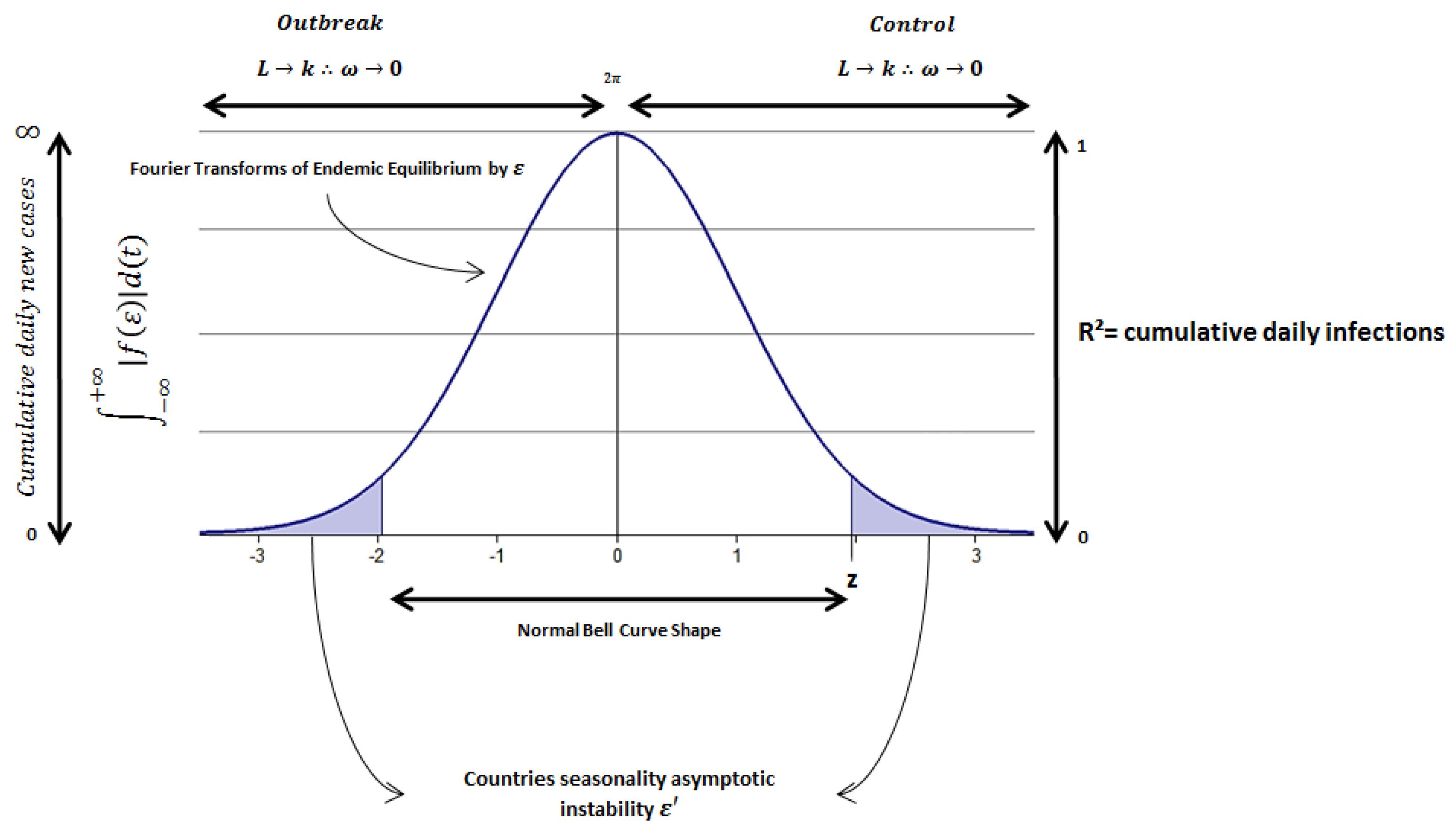
The unexpected seasonality ${\epsilon }^{\prime }$ under heterogeneity forcing behavior explain the exponential behavior of infection spreading patterns among countries an unpredictable sinusoidal expression such as $\beta \left(t\right)={\beta }_0\left(1+\epsilon \varnothing \left(t\right)\right)$, as modelled by Buonuomo et al. [26] with a possibility of using Fourier transforms use, considering finite time lengths of analysis (seasons) equally distributed over the period $T$ within samples (countries). This mathematical framework of analysis applies to the data series of daily new cases when these data present high-amplitude noise, often related to the lower spectral density and lower frequency that makes the analysis imprecise as a sinusoidal stable behavior in the basis form of Earth dissemination seasonality as ${{\displaystyle \int }}_{-\infty }^{+\infty }\left|f\left(\epsilon \right)\right|d\left(t\right)$. In this sense, the sinusoidal behavior does not exist regarding how countries might present default oscillations within seasonal periods of Earth, as represented schematically in Figure 1.

Considering the aspects mentioned before, it is possible to observe that each sample can be understood as the lack of spreading and dissemination patterns towards the confident interval and standard deviation under default periods $T$ from 31 December 2019, to 3 March 2021, resulting in a stochastic maximum exponential form of daily new infections as $Y\left(t\right)$ changes over time, as already observed in the literature [2,8,27,28].

However, despite this scheme pointing to the weaker Earth seasonality forcing behavior of SARS-COV-2 dissemination patterns, it can still influence the overall hidden transmission patterns due to HPALE interventions, environmentally driven seasonality, and urban spaces. This point can be addressed as a pattern formation ${\epsilon }^{\prime }$, of each sample, of confounding forced seasonality that dismantles S and R compartments of SIR predictive model over time [1,27,28,29,30,31,32,33,34], caused by environmental driven factors, urban spaces [35,36,37], and health HPALE intervention [2,3,4,5,6,7,8]. Then, it is possible to observe that each country might respond differently to the same initial conditions [8], influenced by the three components mentioned above, thus generating multiple patterns formation over time $T$ for SARS-CoV-2 forms of transmission and periodicity.

2.4. SIR Model Redefinition from the Original Equation to Skewness Patterns and Global Sensitivity

Concerning a theoretical desired worldwide SIR model normal distribution that most mathematical models imply for infection spreading and dissemination patterns with shape behavior $k=1$ or $k>1$ (Weinbull parameterization) of the exponential “regular” distributions of SARS-CoV-2 infection within time intervals $t$ and with defined periodicity $T$ (possible seasonality forms among countries) [38], the original defined form of $I$ compartment of SIR modeling equation is given as $\frac{dI}{dt}=\beta \frac{SI}{N}-gI$. However, the high asymptotic instability [27,28,29,30,31,32,33,34] of infected individuals ($I$) and the confounding scenario lead to redefining the equation’s basic fundaments to make the skewness analysis. Following this sense, the I compartment of the SIR model was modeled to support confounding data as

$$I={\left(\frac{\omega }{\lambda }\right)}^k$$

(1)

where the infected $I$ is influenced by the unpredictable scale of infection $\lambda$ ($N$) for each sample with inconsistent behavior of variables for S term of the equation, thus influencing the transition rate ($\beta SI$) defined as $\omega$ dissemination patterns (no global solution). Also it is not assumed for $gI$ in the original form of R compartment, that there is a normal distribution output for this virus spreading and dissemination patterns. This new dissemination pattern formation of the epidemic behavior was also described by Duarte et al. [39] when the contact rate does not encompass weather conditions and time-varying aspects of epidemics. Therefore, an unpredictable shape $k$ of probabilistic outcomes (close to reality shapes) was used, mainly defining this shape caused $\lambda$ and $\omega$ asymptotic instabilities generated by S and R compartments over time [1,27,28,29,30,31,32,33,34], among the environmental- and urban space-driven factors [35,36,37] and HPALE interventions [2,3,4,5,6,7,8]. This equation represents the presence of confounding and heterogeneous environmental variables $\omega$ with an unknown predictive scale of $exp\lambda$ or maximum likelihood estimator for $\lambda$ due to non-linear inputs for S and R compartments over time as a global proposition (urban spaces, HPALE, and environmental conditions influence), thus generating nonlinear outputs $k$ (asymptotic instability) [40,41]. If it is considered that most models are searching for a normality behavior among countries, hence, implying that the $k$ distributions are non-complex and not segmented by its partitions, thus resulting in linearity for the virus infection $I$ over $Y$ and $t$, then the overall equation as described by Dietz $\beta \left(t\right)=\beta m\left(1+A\cos \left(\omega t\right)\right)$ [40] would not be reachable for any given period of analysis considering the seasonality forcing behavior of SARS-CoV-2.

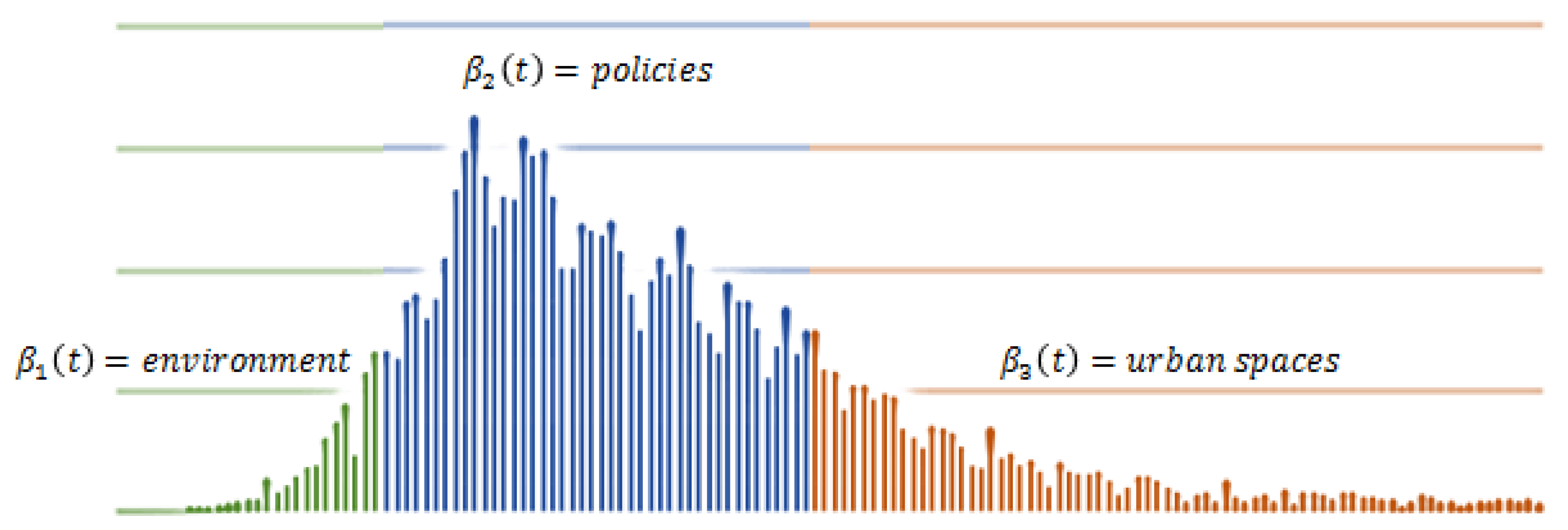
The outputs with heteroscedasticity and non-homologous form for $k$ and $\lambda$ can be modified to reach stable points of analysis, as modelled by Dietz $\beta \left(t\right)=\beta m\left(1+A\cos \left(\omega t\right)\right)$ for each of the three seasonality forces influencing SARS-CoV-2 spreading patterns. These three stable points of the asymptotic structure mentioned before can be observed in Figure 2.

To remove heteroscedasticity and non-homologous form for $k$ and $\lambda$ from occurring in the three phases mentioned in Figure 2, as far as the $\kappa <1$ Weibull parameterization aspect [42] (Bell curve shape) of distribution is chosen as the most reliable region of analysis (attractive orientation) for any given $T$ periods within any sample (countries daily new cases time series), it is necessary to modify the first Equation (1) to

$$I=I={\left(\frac{Y\left(t\right)}{T}\right)}^{k<1}-{\left(\frac{\omega }{\lambda }\right)}^k$$

(2)

hence with the new SIR model proposition as $I=I^{\prime }-\left(S+R\right)$, where $I$ is asymptotic stable to $I^{\prime }$ and S and R considered in its original form $\theta \left(t\right)={\theta }_0\left[1\pm \epsilon \sin \left(2\pi t\right)\right]$ [14]. This is a mandatory redesign since many scientific breakthroughs point to health policies as the best approach to reduce COVID-19 [2,3,4,5,6,7,8]. Starting with this redesign of the equation, it is possible to find one of the first regions of analysis and stability that is health policy intervention, found in the slope (peak) of daily cases over time.

2.5. Birth and Death Persistence of COVID-19 Dissemination Patterns: From Positive to Negative Skew

Considering the new scope of analysis regarding time-series data mentioned before, it is now necessary to uncover the graphic regions in which confounding scenarios can be dismantled with a more robust relation of cause and effect according to Equation (2). It is important to address this birth and death persistence homology for this research, in which the desired mean function $Y\left(t\right)$ of topological space $\mathrm{𝕩}\to \mathbb{R}$ over $\beta \left(t\right)=\beta m\left(1+A\cos \left(\omega t\right)\right)$ indicated at (2) can be found as a persistence diagram existence [43] by mapping each adjacent pair to the point $\left(f\left(Y\right),f\left(t\right)\right)$ local minimum and maximum observations, due to worldwide epidemic growth behaviour and subtle reduction due to HPALE measures. This step results in critical points of $Y$ function over time $t,$ not in adjacent form globally but regionally triangularly space as $d\left(D\left(Y_t\right),D\left(t\right)\right)\le \Vert Y_t-t{\Vert }_{\infty }$ [44] with a given mean region, thus expressing random critical values (dissemination patterns) defined by $I^{\prime }={\left(\frac{Y\left(t\right)}{T}\right)}^{k<1}$ in the real-life form of the event. However, since it is necessary to filter $f\left(Y_n\right)-f\left(t_n\right)=y_n$ unstable critical points (oscillatory instability of seasonality for S and R, HPALE, environmental driven variables, and urban spaces) to an attractive minimum behavior with normal distribution, these regions of analysis must be situated between $\pi <y_n<\frac{\pi }{2}$ for every $A\left(t\right)\to T$ asymptote period. Following this path, and roughly modelling it, the mean $\mu \left(A\left(t\right)\right)$ is obtainable as the size of birth and death persistence diagram and triangulable diagonal ($\Delta$) like $D\left(Y_t,t-\Delta \right)={\displaystyle \sum }_{\pi <y_n<\frac{\pi }{2}}{\mu }_t^{Y_t}$ with multiplicity pairing regions ($t,Y_t$) for each desired triangulation as $0\le t<Y_t\le n+1$, resulting in the general equation for any assumed region as ${\mu }_t^{Y_t}=\beta {\left(t\right)}_{{\epsilon }_{t-1}}^{{\epsilon }_{Y_t}}-\beta {\left(t\right)}_{{\epsilon }_t}^{{\epsilon }_{Y_t}}+\beta {\left(t\right)}_{{\epsilon }_t}^{{\epsilon }_{Y_t}-1}-\beta {\left(t\right)}_{{\epsilon }_{t-1}}^{{\epsilon }_{Y_t}-1}$ [44]. Note that each mean function ${\mu }_t^{Y_t}$ will be given by regions defined as $\beta \left(t\right)=\beta m\left(1+A\cos \left(\omega t\right)\right)$, being $\beta \left(t\right)$ the covariance function of seasonality forcing behavior of dissemination patterns formed by $\mu \left(A\left(t\right)\right)$ under each $\beta \left(t\right)$ form with ${\epsilon }^{\prime }$ partitions, hence without a global mean value for the event in terms of infection and time, or in other words, spreading and dissemination patterns. Further derivations and formulations regarding this persistence diagram will not be addressed for this research. However, it is recommended that future research keep this formulation defined for predictive and monitoring analysis of epidemic seasonality forcing behavior.

It is necessary to understand that this new design of seasonality regions can now be adapted adequately to Fourier transform analysis under the amplitude of waves with the equation $e^{-i\omega t}=\cos \left(2\pi t\right)+i \sin \left(2\pi t\right)$ where angular momentum was drawn in the limits of $\beta \left(t\right)=\beta m\left(1+A\cos \left(\omega t\right)\right)$, giving $\omega =\pi <y_n<\frac{\pi }{2}$ and generally defining it with sinusoidal reduced form as $f\left({ϵ}^{\prime }\right)={{\displaystyle \int }}_{-\infty }^{+\infty }Y\left(t\right)e^{-2\pi i\omega t}d\omega$ to reach a sinusoidal approach of time series data extraction and analysis over periods ${\epsilon }^{\prime }$ and given analysis regions.

Beyond the limitation of periods for predictive analysis and monitoring as a Gaussian process in the overall data of the given epidemics, the design in this article introduces one main point of analysis that is the lack of a global mean and covariance function $\mu \left(Y\left(t\right)\right)$ over fluctuations as a global homomorphism and a decomposition form of wave signals similar to Fourier transforms. This occurs since spreading patterns of infection find heterogeneity within the type of HPALE interventions influenced by the confounding scenario created by the environment and urban spaces where persistent homology and homotopy cannot be found for $t\therefore \kappa <1$ Weibull reliability to be situated globally for the overall times series data of epidemics in the oscillation-pairing regions of $\sin \left(\pi \right)=1$ and $\cos \left(\pi \right)=0$ for $T$ desired coordinates of persistent fluctuations in $\left(f\left(Y_n\right),f\left(t_{k<1}\right)\right)=y_n$ of stability can differ over an extended time of analysis. HPALE range of influence is no longer stable (weak boundaries points of persistence), and therefore assuming $t+1$ discrete form, defined as $y_n=f\left(f\left(Y_n\right),f\left(t_{k<1}\right)\right){{\displaystyle \int }}_{\frac{\pi }{2}}^{\pi }\mu {\displaystyle \sum }\left(Y_0,\dots , Y_n\right)dt$. However, by contrast, it can be found with continuous form as $\delta =f\left(Y_t,t\right){{\displaystyle \int }}_{\frac{\pi }{2}}^{\pi }\mu {\displaystyle \sum }\left(Y_0,\dots ,Y_n\right)d\mu$ [9], thus assuming the shape and limit to $\kappa <1$ as small partitions ${\epsilon }^{\prime }$ to the desired analysis or without a derivative form for the overall analysis within the whole epidemics behavior observed. Considering the new partitions ${\epsilon }^{\prime }$, for the discretized view of $Y_t,t$ as pointed out in the results of Roberts et al. [9], it is now possible to obtain a sample mean as a mode like $\overline{\mu }=\frac{1}{n}{\displaystyle \sum }_i^n{Y}_t,t$. Further results of this approach can be visualized at [9] Roberts et al. reference.

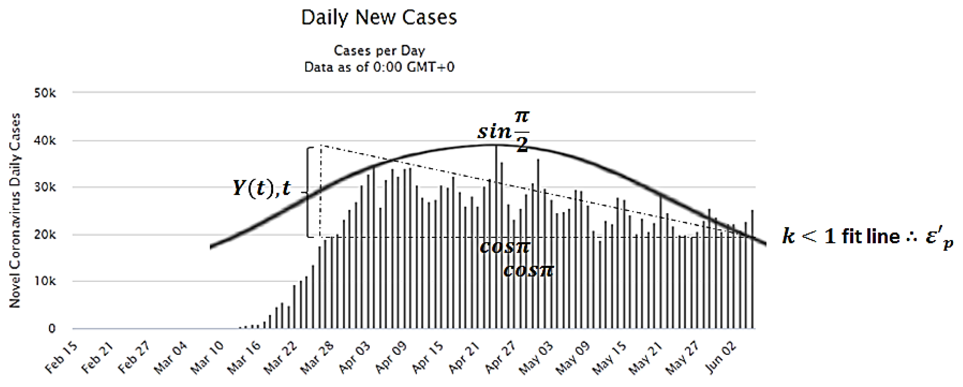
By rejecting the persistence diagram’s unstable critical points generated globally, a local minimum of the event as an average mean ${\epsilon }^{\prime }$ can be obtained by having $Y\left(t\right)$ with the higher number of samples $Y$ (daily infections) that finds a condition roughly described in the nonlinear oscillations within the exponential growth epidemic behavior of event as limited between maximum local growth defined by $\frac{\pi }{2}$ by its half curvature oscillations $\pi$ as a local minimum being non-periodic as $2\pi$ in a global homomorphism sense due to $\kappa <1$. In this sense, the new sinusoidal approach offers a new mean function as an angular momentum of $=\pi <y_n<\frac{\pi }{2}$, hence the wave-signal necessary to perform the Fourier transforms in each ${\epsilon }^{\prime }$ of data. This scheme can be observed for HPALE intervention on SARS-CoV-2 spreading and dissemination patterns [27] in Figure 3.

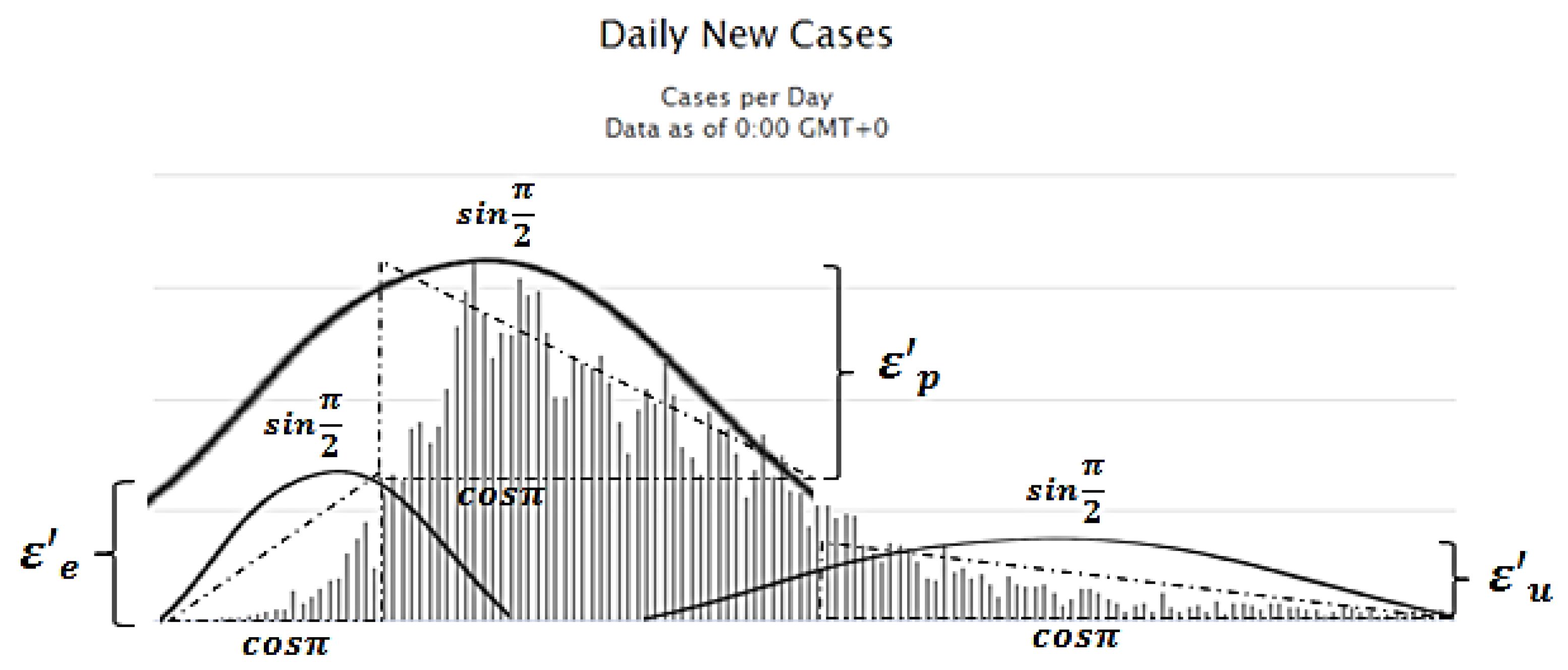
Therefore, $Y\left(t\right),t$ assumes the desired oscillations samples and region conditions ${\epsilon }^{\prime }$ as $\pi <y_n<\frac{\pi }{2}$ where birth and death persistent homology can be found for $t\therefore \kappa <1$ to be situated in the oscillations pairing region of $\sin \left(\pi \right)=0$ and $\cos \left(\pi \right)=Y\left(t\right)$ for $Y\left(t\right),t$ desired coordinates $\left(f\left(Y\left(t\right)\right),f\left(t\right)\right)$ of stability with discrete form as $t+1$ as $Y\left(t\right)=f\left(Y\left(t\right)\right){{\displaystyle \int }}_{\frac{\pi }{2}}^{\pi }\mu {\displaystyle \sum }\left(Y_0,\dots ,Y_n\right)dt$ or vice-versa for $t=f\left(t\right){{\displaystyle \int }}_{\frac{\pi }{2}}^{\pi }\mu {\displaystyle \sum }\left(t_0,\dots ,t_n\right)d{Y}_t$, thus assuming the shape and limit to $\kappa <1$. Considering samples’ time lengths, it is designed as $t\left(\delta +1\right)\le f\left(Y\left(t\right)\right)\mu {\displaystyle \sum }\left(Y_0,\dots ,Y_n\right)dt$ starting from $t_0,\dots ,t_n\le \sin \left(\frac{\pi }{2}\right)$ results in the desired data distribution with a conditional shape of Weibull parameterization $\kappa <1$ for the analysis with a normal distribution, thus rejecting any critical value beyond $\cos \left(\pi \right)={{\epsilon }^{\prime }}_p$ and under $\sin \left(\pi \right)={{\epsilon }^{\prime }}_p$, being ${{\epsilon }^{\prime }}_p$ the seasonality forcing behavior of HPALE intervention over SARS-CoV-2 among countries’ data sets. Concerning time lengths of samples, designed as $t\left(y_n+1\right)\le f\left(Y_n\right)\mu {\displaystyle \sum }\left(Y_0, \dots , Y_n\right)dt$ starting from $t_0,\dots ,t_n\le \sin \left(\pi \right)$ results in the desired data distribution, thus rejecting any critical value beyond $\cos \left(\pi \right)=0$ and under $\sin \left(\pi \right)=1$. The main reason to ignore S and R local solutions, or to not use SIR models globally, is also the same reason to adopt a region of analysis in the time series data for $I^{\prime }$ and HPALE.This also remains for the other two important inputs of the system derivatives (environmental factors that influence COVID-19 dissemination and urban spaces) of which for each country the aforementioned confounding scenario of analysis is shown in Figure 4.

Noting that the S and R compartments of the SIR model are needed for predictive analysis of infection dissemination patterns, these compartments might work properly under the third region of time series data: urban spaces ${{\epsilon }^{\prime }}_u$ seasonality. To achieve results with a high uncertainty reduction, it is necessary to conceive S and R as in its most stable region of analysis, which should be influenced in a posterior scenario where ${{\epsilon }^{\prime }}_p$ (HPALE) and ${{\epsilon }^{\prime }}_e$ (environmental seasonality) already took effect. This is mandatory since, as far as policies are assumed in models or estimated with unreal quantitative parameters, uncertainty growth is promoted along with limitations to track real patterns within an urban space feature for S and R as a causation relation. For urban spaces seasonality forcing behavior, it is considered that inside and outside urban spaces promote limitations to HPALE due to the limiting action that it can face within these urban spaces (not all HPALE can reach some urban spaces features properly as it was designed to be). Environmental seasonality can also be present at this phase by influencing urban spaces limitations of taken HPALE actions. Therefore, ${{\epsilon }^{\prime }}_e$ might find a growing point inside and outside urban spaces beyond ${{\epsilon }^{\prime }}_p$ normalization (more explanation of this causation effect will be given in the Results section), which can be the cause of worldwide second waves or posterior waves.

Considering unexpected seasonal forcing ${{\epsilon }^{\prime }}_p$ roughly defined as $\partial \left(t\right)={\partial }_0\left[1\pm {\epsilon }_0\cos \pi <{\epsilon }^{\prime }<\sin \frac{\pi }{2}\right]$ [9] in a complex network model, where no periodic oscillation (sinusoidal) are to be found in a discrete form with $f\left({{\epsilon }^{\prime }}_{e,p,u}\right)={{\displaystyle \int }}_{-\infty }^{+\infty }Y\left(t\right),t{e}^{-2\pi i\omega t}d\omega$, assume now a rupture of the $\sin \left(2\pi t\right)$, leaving the region the pre-assumed linearity $\theta \left(t\right)={\theta }_0\left[1\pm \epsilon \sin \left(2\pi t\right)\right]$ for S and R in the overall metrics of time series data $T$ within one sample or among countries and understanding each iteration of the event as unconnected to the previous and future data if considering multiple time-series comparisons (among countries) or even in the same time series if considering long-term analysis. Since the $I^{\prime }$ is an asymptote to ${{\epsilon }^{\prime }}_p$, then ${{\epsilon }^{\prime }}_u$ is limited by ${{\epsilon }^{\prime }}_p$ on $I^{\prime }$, but not necessarily fully stable in terms of ${{\epsilon }^{\prime }}_p$ present total control over environmental seasonality due to urban space features.

It is possible to verify that most of these SIR models are constructed based on ${{\epsilon }^{\prime }}_p$ seasonality behaviors [45,46,47,48]. Following this phase, urban spaces and HPALE interventions might present a strong influence on the outcomes due to the unpredictability of S and R patterns to design appropriate contact rates, which still represents a limitation for the SIR model methods [27,28,29,30,31,32,33,34]. Nonetheless, it is still the most desirable region of analysis for data extraction.

3. Results

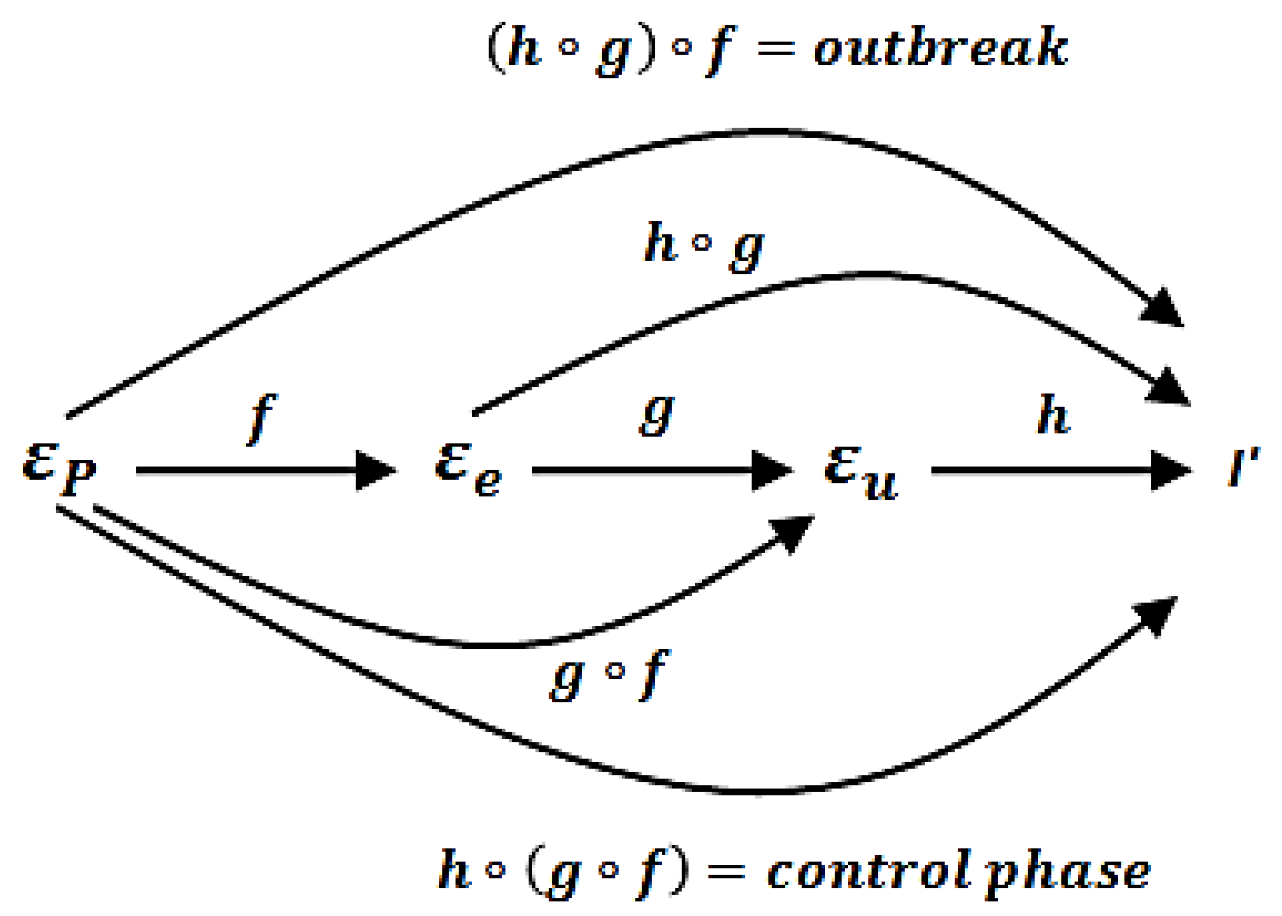
The overall scenario of spreading and dissemination patterns skewness concerning the environment, HPALE and urban spaces can be visualized in Figure 5, where seasonality forcing behavior assumes the following topological metric space. Considering all the possible seasonality types, $f\left({{\epsilon }^{\prime }}_{e,p,u}\right)={{\displaystyle \int }}_{-\infty }^{+\infty }Y\left(t\right),t{e}^{-2\pi i\omega t}d\omega$, in continuous form of observation, with the need to discretize within causal roots of analysis due to heterogeneity and confounding scenario of analysis, HPALE seasonality can be understood as $f{{\epsilon }^{\prime }}_p=g\circ f\left(Y_t,t\right)=g\left(f\left({{\epsilon }^{\prime }}_p\right)\right)$, hence it can also be written as, $f{{\epsilon }^{\prime }}_p=h\circ \left(g\circ f\left(Y_t,t\right)\right)=h\left(g\left(f\left({{\epsilon }^{\prime }}_p\right)\right)\right)$ as a control phase of local epidemics. However, this phase might present high instability (spreading patterns fluctuations) at a worldwide level due to heterogeneity and confounding behavior of $f{{\epsilon }^{\prime }}_u$ and $f{{\epsilon }^{\prime }}_e$. Since SIR models require stable points for S and R, there is $f{{\epsilon }^{\prime }}_u=h\circ g\left(Y_t,t\right)=h\left(g\left({{\epsilon }^{\prime }}_u\right)\right)$, resulting in a stable asymptotic convergence only if $f{{\epsilon }^{\prime }}_p=h\circ \left(g\circ f\left(Y_t,t\right)\right)=h\left(g\left(f\left({{\epsilon }^{\prime }}_p\right)\right)\right)$. Since the outbreak might incur in unknown spreading and dissemination patterns for $f{{\epsilon }^{\prime }}_p$, $f{{\epsilon }^{\prime }}_e$ and $f{{\epsilon }^{\prime }}_u$, this region needs to be carefully considered. Therefore, environmental seasonality can be found as $f{{\epsilon }^{\prime }}_e=\left(h\circ g\left(Y_t,t\right)\right)\circ f=f\left(h\left(g\left({{\epsilon }^{\prime }}_e\right)\right)\right)$ or it is also possible to assume $f{{\epsilon }^{\prime }}_e=(\epsilon \circ g\left(Y_t,t\right)$, being $\epsilon$ the undefined patterns of environmentally driven new infections for Earth seasonality or atmospheric factors, which was not fully resolvable in this research.

4. Discussion

Concerning urban spaces’ spreading patterns, due to the vast diversity of public health infrastructure buildings design, outdoor and indoor building designs within natural physical features such as rivers, lakes, snow, culture, and urbanization developments, they exert influence on the region of environmental driven pattern and not only policies. Therefore, it is reasonable to understand that any assumption on S and R during the epidemic phase in its initial curvature is much more closed to uncertainty measures than ever due to several possible confluences. Countries may then diverge greatly in the urban space and environmental scenarios, and thus S and R compartments face calculation limitations during peak curvature, being uncertain how to predict virus spreading and dissemination patterns since policies/HPALE are not even fully developed or had adequate time to take effect while most of the models use policies as the basis of modeling the dissemination patterns. For this reason, the most reliable region of analysis for these compartments and where most of the models are currently situated/functioning remains at the control phase of epidemics. However, fluctuations may still occur worldwide due to the type of HPALE and urban space features. Therefore, urban spaces and environmental seasonality drivers are the main cause of aperiodic and unstable behavior for SARS-COV-2 spreading patterns worldwide. It is likely that environmental driven seasonality results found in many studies are, in truth, HPALE and urban spaces results, representing a need for further detailed research [48].

This was addressed in the research [49], where despite the vast review made, and the observation of confounding scenarios for each sample of analysis and type of climate conditions that influence COVID-19 spreading patterns, authors [49] have understood that there are homogeneity and heterogeneity in the statistical results and conclusions about the environmental influence on the virus dissemination patterns. This was addressed correctly in a systematic review [49] and further developed in this present study through a careful observation that environmental influence can be better understood in outbreaks and urban spaces by using graph analysis. Also, despite the analysis made in [49] considering only policies and climate conditions, further scenario need to be evaluated that is urban spaces, where human lifestyles are directly connected with a risk behaviour over contamination of infectious diseases, such as COVID-19, hence human behaviours also have great impact in the preventive measures efficacy.

Also, concerning evolutionary and game of life algorithms [50,51], predefined parameters and initial inputs are crucial for the machine learning analysis. However, beyond biological features as described in the last paragraph, unpredictable scale of infected individuals are found worldwide without vaccination or social isolation. The article aimed to analyze the problem without these predefined parameters being the basis and sensitivity of analysis. This can be mandatory since many countries are facing problems with vaccination speed and availability as well as social isolation as well as a severe lack of citizen compliance in many countries. Similarly, in Bateman SIZ analysis, this approach can be observed [52] regarding the uncertainty of models without using predefined parameters for sensitivity and robustness. These uncertain parameters lead the calculations to include new panoramic idea of how to combat COVID-19 without proper pre assumptions, thus giving for the real world skewness observed in predictive methods, a degree of uncertainty worldwide. This can be useful due to the lack of correlation between the sensitivity of models and real life complexity.

Concerning uncertainty and sensitivity, the article presents some references that address this point [8,30,33,45]. This research’s main objective was to analyse the SIR model equation without pre-defined data input in terms of formulating a specific SIR model to perform predictive analysis with numerical results. For this reason, theoretical observations were made, considering references findings and the global sensitivity model used (policies and ALE, environment and urban spaces). Despite not considering numerical solutions of the problem, due to complexity issues for data collection in real life and chaotic behaviour of some events, the theoretical model proposed can be helpful to understand how pandemics should be investigated for future SIR model equations and also for the basic interpretation of epidemiological behaviour of SARS-COV-2. This is mandatory nowadays since many countries present unfitted vaccination prediction, unfitted social isolation prediction and unfitted SARS-COV-2 variants appearance. The validation of the data subject can be found in Section 2.2. Skewness validation and SIR model limitation. Since the model proposed in this article is not developed to numerical data or results, the theoretical basis of analysis was retrieved from references that already performed these numerical solutions of the problem. Therefore, compiling these findings, it was possible to observe how skewness properties of the issue express how the virus behaves worldwide without predefined spreading and dissemination patterns. This concept of an absence of predefined spreading and dissemination patterns was supported in the results section, aiming to describe how uncertainty and predictive constraints can be found based on the SIR model equation and its variants developed worldwide.

In the research results section, it is possible to observe that the most reliable region to investigate environmental seasonality remains at the outbreak and control phases. In contrast, best urban space seasonality observations remain at the control phase. This feature can be very useful for HPALE approaches since the actual fluctuations/instability in the region mentioned above are mainly caused by these two posterior forcing behaviors. Therefore, new strategies and measurements need to be adopted to keep the economy and prevention with similar power, which was already initially investigated by Sajadi et al. in June 2020 [46].

Note that there is a great difference between environment-driven seasonality caused by urban spaces influenced by HPALE limitations or otherwise caused by Earth and other natural (atmospheric) seasonality forcing behavior at outbreaks. This characteristic should be carefully considered when studying Earth seasonality among countries. The compartmental models are mostly in the control phase region and lose efficacy at outbreaks where no specific parameters are given, and environmental seasonality is not yet discovered in its true patterns. Another point regarding the control phase is that in which instabilities can occur, as far as urban spaces create a scenario where HPALE faces limitations, environmental seasonality finds a suitable place to grow its patterns [47]. Due to uncertainty growth over time and the lack of mean for defined intervals of $t$ over $T$ normal distribution shape for the whole data, Earth season $\epsilon$ gradually loses its effect with the possibility of random delays observed for each country of analysis (sample) being attributed by different patterns in which an outbreak occurs since existing HPALE are found within worldwide cultures, science, and education.

5. Conclusions

This research modeled SARS-COV-2 spreading and dissemination patterns sensitivity by defining and redesigning time series data extraction to SIR model equations. The approach opened a new scenario where seasonality forcing behavior was introduced to understand SARS-COV-2 skewness expressions due to heterogeneity and confounding epidemics scenarios where actual SIR models might find a high degree of uncertainty caused by oscillatory conditions found in the input of variables of the event.

The main research results are the elucidation of three birth and death forced seasonality phases that can explain how COVID-19 spreading and dissemination patterns skewness occurs worldwide. It can be understood in the following order: (1) the environmental variables (Earth seasons and atmospheric conditions); (2) health policies and adult learning education (HPALE) interventions; (3) urban spaces (local indoor and outdoor spaces for transit and social-cultural interactions, public or private, with natural physical features (river, lake, terrain).

These three forced seasonality phases were pointed to as the most effective explanation concerning uncertainty found in the predictive SIR model equations that might diverge in outcomes expected to express the disease’s behaviour. Therefore, many distinct models were generated to cover COVID-19 confounded scenarios.

Regarding the forced seasonality model the following pattern was observed: HPALE can be the strongest stable point of seasonality during the epidemic peak phase and compartmental models are influenced mainly by HPALE, while environmental and urban spaces present a low or hidden influence on it. However, HPALE can still be limited at the control phase, depending on urban spaces and existing environmental conditions demanding SIR models to adapt to these new features. Finally, at outbreak and control phases, environmental factors present outcomes caused by the existing HPALE and urban spaces of a given sample, thus producing high uncertainty to predictive SIR model equations.

6. Limitations

ALE was considered in the view of effective practice mainly based on adequate policies adopted by countries. Nonetheless, it should be carefully addressed in the view of infodemics practices, in which ALE can assume one more seasonal force in epidemics, disrupting the peak and control phase and promoting new spreading and dissemination patterns during ${{\epsilon }^{\prime }}_p$ seasonality. It can also enforce posterior waves and confirm spreading pattern fluctuations at outbreaks and urban spaces’ stability and. therefore. demanding new modifications in SIR models.

References

- Grassly, N.C.; Fraser, C. Seasonal infectious disease epidemiology. Proc. R. Soc. B Biol. Sci. R. Soc. 2006, 273, 2541–2550. [Google Scholar] [CrossRef] [PubMed] [Green Version]
- Su, D.; Chen, Y.; He, K.; Zhang, T.; Tan, M.; Zhang, Y.; Zhang, X. Influence of Socio-Ecological Factors on COVID-19 Risk: A Cross-Sectional Study Based on 178 Countries/Regions Worldwide. SSRN Electron. J. 2020. [Google Scholar] [CrossRef]
- Telles, C.R.; Roy, A.; Ajmal, M.R.; Mustafa, S.K.; Ahmad, M.A.; de la Serna, J.M.; Frigo, E.P.; Rosales, M.H. Influence of countries adopted social distancing policy for COVID-19 reduction under the view of the airborne transmission framework (Preprint). JMIR Public Heal Surveill. 2020, 11. [Google Scholar] [CrossRef]
- Block, P.; Hoffman, M.; Raabe, I.J.; Dowd, J.B.; Rahal, C.; Kashyap, R.; Mills, M.C. Social network-based distancing strategies to flatten the COVID-19 curve in a post-lockdown world. Nat. Hum. Behav. 2020, 4, 588–596. [Google Scholar] [CrossRef] [PubMed]
- Ferguson, N.; Laydon, D.; Nedjati Gilani, G.; Imai, N.; Ainslie, K.; Baguelin, M.; Bhatia, S.; Boonyasiri, A.; Cucunuba Perez, Z.U.; Cuo-mo-Dannenburg, G.; et al. Report 9: Impact of Non-Pharmaceutical Interventions (NPIs) to Reduce COVID19 Mortality and Healthcare Demand; Imperial College London: London, UK, 2020. [Google Scholar] [CrossRef]
- Chu, D.K.; Akl, E.A.; Duda, S.; Solo, K.; Yaacoub, S.; Schünemann, H.J.; El-Harakeh, A.; Bognanni, A.; Lotfi, T.; Loeb, M.; et al. Physical distancing, face masks, and eye protection to prevent person-to-person transmission of SARS-CoV-2 and COVID-19: A systematic review and meta-analysis. Lancet 2020, 395, 1973–1987. [Google Scholar] [CrossRef]
- Lopes, H.; McKay, V. Adult learning and education as a tool to contain pandemics: The COVID-19 experience. Int. Rev. Educ. 2020, 66, 575–602. [Google Scholar] [CrossRef]
- Alberti, T.; Faranda, D. On the uncertainty of real-time predictions of epidemic growths: A COVID-19 case study for China and Italy. Commun. Nonlinear Sci. Numer. Simul. 2020, 90, 105372. [Google Scholar] [CrossRef] [PubMed]
- Roberts, M.; Andreasen, V.; Lloyd, A.; Pellis, L. Nine challenges for deterministic epidemic models. Epidemics 2015, 10, 49–53. [Google Scholar] [CrossRef] [PubMed] [Green Version]
- Dong, E.; Du, H.; Gardner, L. An interactive web-based dashboard to track COVID-19 in real time. Lancet Infect. Dis. 2020, 20, 533–534. [Google Scholar] [CrossRef]
- Altizer, S.; Dobson, A.; Hosseini, P.; Hudson, P.; Pascual, M.; Rohani, P. Seasonality and the dynamics of infectious diseases. Ecol. Lett. 2006, 9, 467–484. [Google Scholar] [CrossRef] [Green Version]
- Bacaër, N.; Dads, E.H.A. On the biological interpretation of a definition for the parameter R 0 in periodic population models. J. Math. Biol. 2011, 65, 601–621. [Google Scholar] [CrossRef] [PubMed]
- Siettos, C.I.; Russo, L. Mathematical modeling of infectious disease dynamics. Virulence 2013, 4, 295–306. [Google Scholar] [CrossRef] [PubMed] [Green Version]
- Mari, L.; Casagrandi, R.; Bertuzzo, E.; Rinaldo, A.; Gatto, M. Floquet theory for seasonal environmental forcing of spatially explicit waterborne epidemics. Theor. Ecol. 2014, 7, 351–365. [Google Scholar] [CrossRef] [Green Version]
- Zhang, Y.; You, C.; Cai, Z.; Sun, J.; Hu, W.; Zhou, X.H. Prediction of the COVID-19 outbreak based on a realistic stochastic model. medRxiv 2020. [Google Scholar] [CrossRef] [Green Version]
- Utsunomiya, Y.T.; Utsunomiya, A.T.H.; Torrecilha, R.B.P.; Paulan, S.D.C.; Milanesi, M.; Garcia, J.F. Growth Rate and Acceleration Analysis of the COVID-19 Pandemic Reveals the Effect of Public Health Measures in Real Time. Front. Med. 2020, 7, 247. [Google Scholar] [CrossRef] [PubMed]
- Stübinger, J.; Schneider, L. Epidemiology of Coronavirus COVID-19: Forecasting the Future Incidence in Different Countries. InHealthcare 2020, 8, 99. [Google Scholar] [CrossRef] [Green Version]
- Rock, K.; Brand, S.; Moir, J.; Keeling, M.J. Dynamics of infectious diseases. Rep. Prog. Phys. 2014, 77, 026602. [Google Scholar] [CrossRef]
- Billings, L.; Schwartz, I.B. Exciting chaos with noise: Unexpected dynamics in epidemic outbreaks. J. Math. Biol. 2002, 44, 31–48. [Google Scholar] [CrossRef] [PubMed]
- WHO. World Health Organization: Influenza Laboratory Surveillance Information by the Global Influenza Surveillance and Response System (GISRS). Available online: https://www.who.int/influenza/gisrs_laboratory/flunet/charts/en/ (accessed on 25 June 2020).
- Li, Y.; Wang, X.; Nair, H. Global Seasonality of Human Seasonal Coronaviruses: A Clue for Postpandemic Circulating Season of Severe Acute Respiratory Syndrome Coronavirus 2? J. Infect. Dis. 2020, 222, 1090–1097. [Google Scholar] [CrossRef] [PubMed]
- Smit, A.J.; Fitchett, J.M.; Engelbrecht, F.A.; Scholes, R.J.; Dzhivhuho, G.; Sweijd, N.A. Winter Is Coming: A Southern Hemisphere Perspective of the Environmental Drivers of SARS-CoV-2 and the Potential Seasonality of COVID-19. Int. J. Environ. Res. Public Health 2020, 17, 5634. [Google Scholar] [CrossRef]
- Engelbrecht, F.A.; Scholes, R.J. Test for Covid-19 seasonality and the risk of second waves. One Health 2021, 12, 100202. [Google Scholar] [CrossRef]
- Kanzawa, M.; Spindler, H.; Anglemyer, A.; Rutherford, G.W. Will Coronavirus Disease 2019 Become Seasonal? J. Infect. Dis. 2020, 222, 719–721. [Google Scholar] [CrossRef]
- Grenfell, B.; Kleczkowski, A.; Gilligan, C.; Bolker, B. Spatial heterogeneity, nonlinear dynamics and chaos in infectious diseases. Stat. Methods Med. Res. 1995, 4, 160–183. [Google Scholar] [CrossRef]
- Buonomo, B.; Chitnis, N.; D’Onofrio, A. Seasonality in epidemic models: A literature review. Ric. Mat. 2018, 67, 7–25. [Google Scholar] [CrossRef]
- Telles, C.R. Reducing SARS-CoV-2 infectious spreading patterns by removing S and R compartments from SIR model equa-tion. medRxiv 2020. [Google Scholar] [CrossRef]
- Carlson, C.J.; Gomez, A.C.R.; Bansal, S.; Ryan, S.J. Misconceptions about weather and seasonality must not misguide COVID-19 response. Nat. Commun. 2020, 11, 1–4. [Google Scholar] [CrossRef] [PubMed]
- Manzo, G. Complex social networks are missing in the dominant covid-19 epidemic models. Sociologica 2020, 14, 31–49. [Google Scholar] [CrossRef]
- Merchant, H. CoViD-19 may not end as predicted by the SIR model. BMJ 2020, 369. Available online: https://www.bmj.com/content/369/bmj.m1567/rr (accessed on 30 April 2020).
- Adam, D. The simulations driving the world’s response to covid-19. How epidemiologists rushed to model the corona-virus pandemic. Nature 2020, 580, 316–318. [Google Scholar] [CrossRef] [Green Version]
- Luo, J. Predictive Monitoring of COVID-19; SUTD Data-Driven Innovation Lab.: Singapore, 2020. [Google Scholar]
- Best, R.; Boice, J. Where The Latest COVID-19 Models Think We’re Headed—And Why They Disagree. Abc News: FiveThir-tyEight. Available online: https://projects.fivethirtyeight.com/covid-forecasts/ (accessed on 11 June 2020).
- Koerth, M.; Bronner, L.; Mithani, J. Why It’s So Freaking Hard to Make a Good COVID-19 Model. Abc News: FiveThirtyEight. Available online: https://fivethirtyeight.com/features/why-its-so-freaking-hard-to-make-a-good-covid-19-model/ (accessed on 31 March 2020).
- Liu, Y.; Ning, Z.; Chen, Y.; Guo, M.; Liu, Y.; Gali, N.K.; Sun, L.; Duan, Y.; Cai, J.; Westerdahl, D.; et al. Aerodynamic analysis of SARS-CoV-2 in two Wuhan hospitals. Nat. Cell Biol. 2020, 582, 557–560. [Google Scholar] [CrossRef] [PubMed]
- Lin, K.; Marr, L.C. Humidity-Dependent Decay of Viruses, but Not Bacteria, in Aerosols and Droplets Follows Disinfection Kinetics. Environ. Sci. Technol. 2020, 54, 1024–1032. [Google Scholar] [CrossRef] [PubMed]
- Morawska, L.; Milton, D.K. It Is Time to Address Airborne Transmission of Coronavirus Disease 2019 (COVID-19). Clin. Infect. Dis. 2020. [Google Scholar] [CrossRef]
- Roda, W.C.; Varughese, M.B.; Han, D.; Li, M.Y. Why is it difficult to accurately predict the COVID-19 epidemic? Infect. Dis. Model. 2020, 5, 271–281. [Google Scholar] [CrossRef]
- Duarte, J.; Januário, C.; Martins, N.; Rogovchenko, S.; Rogovchenko, Y. Chaos analysis and explicit series solutions to the seasonally forced SIR epidemic model. J. Math. Biol. 2019, 78, 2235–2258. [Google Scholar] [CrossRef] [PubMed]
- Dietz, K. The Incidence of Infectious Diseases under the Influence of Seasonal Fluctuations. In Mathematical Models in Medicine; Springer: Berlin, Germany, 1976; pp. 1–15. [Google Scholar] [CrossRef]
- Telles, C.R. False asymptotic instability behavior at iterated functions with Lyapunov stability in nonlinear time series. In Science and Information Conference; Springer: Cham, Switzerland, 2020; pp. 673–693. [Google Scholar] [CrossRef]
- Jiang, R.; Murthy, D.N. A study of Weibull shape parameter: Properties and significance. Reliab. Eng. Syst. Saf. 2011, 96, 1619–1626. [Google Scholar] [CrossRef]
- Edelsbrunner, H.; Harer, J. Persistent homology-a survey. Contemp. Math. 2008, 453, 257–282. Available online: https://www.maths.ed.ac.uk/~v1ranick/papers/edelhare.pdf (accessed on 14 July 2020).
- Cohen-Steiner, D.; Edelsbrunner, H.; Harer, J. Stability of persistence diagrams. Discret. Comput. Geom. 2007, 37, 103–120. Available online: http://math.uchicago.edu/~shmuel/AAT-readings/Data%20Analysis%20/Edelsbrunner,%20Harer,%20Stability.pdf (accessed on 25 August 2020). [CrossRef] [Green Version]
- CDC. Centers for Disease Control and Prevention. CASES, DATA & SURVEILLANCE: Forecasts of Total Deaths July 2, 2020. Available online: https://www.cdc.gov/coronavirus/2019-ncov/covid-data/forecasting-us.html (accessed on 8 July 2020).
- Sajadi, M.M.; Habibzadeh, P.; Vintzileos, A.; Shokouhi, S.; Miralles-Wilhelm, F.; Amoroso, A. Temperature, Humidity, and Latitude Analysis to Estimate Potential Spread and Seasonality of Coronavirus Disease 2019 (COVID-19). JAMA Netw. Open 2020, 3, e2011834. [Google Scholar] [CrossRef] [PubMed]
- Lin, J.; Huang, W.; Wen, M.; Li, D.; Ma, S.; Hua, J.; Hu, H.; Yin, S.; Qian, Y.; Chen, P.; et al. Containing the spread of coronavirus disease 2019 (COVID-19): Meteorological factors and control strategies. Sci. Total. Environ. 2020, 744, 140935. [Google Scholar] [CrossRef] [PubMed]
- Rucinski, S.L.; Binnicker, M.J.; Thomas, A.S.; Patel, R. Seasonality of Coronavirus 229E, HKU1, NL63, and OC43 from 2014 to 2020. In Mayo Clinic Proceedings; Elsevier BV: Amsterdam, The Netherlands, 2020; Volume 95, pp. 1701–1703. [Google Scholar]
- Mecenas, P.; Bastos, R.T.D.R.M.; Vallinoto, A.C.R.; Normando, D. Effects of temperature and humidity on the spread of COVID-19: A systematic review. PLoS ONE 2020, 15, e0238339. [Google Scholar] [CrossRef]
- Ghosh, S.; Bhattacharya, S. A data-driven understanding of COVID-19 dynamics using sequential genetic algo-rithm based probabilistic cellular automata. Appl. Soft Comput. 2020, 96, 106692. [Google Scholar] [CrossRef]
- Machado, J.A.T. An Evolutionary Perspective of Virus Propagation. Mathematics 2020, 8, 779. [Google Scholar] [CrossRef]
- Braun, P.; Haffner, S.; Woodcock, B.G. COVID-19 pandemic predictions using the modified Bateman SIZ model and observational data for Heidelberg, Germany: Effect of vaccination with a SARS-CoV-2 vaccine, coronavirus testing and application of the Corona-Warn-App. Int. J. Clin. Pharmacol. Ther. 2020, 58, 417–425. [Google Scholar] [CrossRef] [PubMed]
Figure 1.
General framework of coronavirus disease 2019 (COVID-19) seasonality under the view of Fourier transform use limitations.
Figure 2.
Severe acute respiratory syndrome coronavirus 2 (SARS-COV-2) spreading and dissemination patterns filtered and stated as expressing within the three phases of the epidemic: environmental spreading and dissemination patterns, health policies and adult learning education (HPALE), and the urban spaces dissemination patterns.
Figure 3.
HPALE stable region of analysis on SARS-CoV-2 dissemination patterns. Image data source: Worldometer—Italy on 8 July 2020.
Figure 4.
Considering the observation COVID-19 confounding scenario, it is presented the asymptotic strong seasonality force of HPALE () intervention and the narrow and unstable region (outbreak and control) of analysis for environmental and urban driving factors of seasonality ( ).
Figure 5.
Schematically representation of the COVID-19 skewness properties: during epidemics evolution, HPALE influences the environment and urban spaces seasonality until a limit defined by its type and strategy of application; compartmental models during peak phase are influenced by HPALE, environment and urban spaces and present high uncertainty; at control phase, policies/HPALE finds its limitation by the environment and the type of urban spaces and finally, at outbreak, environmental factors present outcomes caused by the existing HPALE and urban spaces.
Publisher’s Note: MDPI stays neutral with regard to jurisdictional claims in published maps and institutional affiliations. |
© 2021 by the authors. Licensee MDPI, Basel, Switzerland. This article is an open access article distributed under the terms and conditions of the Creative Commons Attribution (CC BY) license (https://creativecommons.org/licenses/by/4.0/).
Share and Cite
MDPI and ACS Style
Roberto Telles, C.; Lopes, H.; Franco, D. SARS-COV-2: SIR Model Limitations and Predictive Constraints. Symmetry 2021, 13, 676. https://doi.org/10.3390/sym13040676
AMA Style
Roberto Telles C, Lopes H, Franco D. SARS-COV-2: SIR Model Limitations and Predictive Constraints. Symmetry. 2021; 13(4):676. https://doi.org/10.3390/sym13040676
Chicago/Turabian StyleRoberto Telles, Charles, Henrique Lopes, and Diogo Franco. 2021. "SARS-COV-2: SIR Model Limitations and Predictive Constraints" Symmetry 13, no. 4: 676. https://doi.org/10.3390/sym13040676
Note that from the first issue of 2016, this journal uses article numbers instead of page numbers. See further details here.