Investigating the Impact of Regional Temperature on COVID-19 Pandemic during 2020

Abstract

Several studies have attempted to uncover the impact of weather parameters on the coronavirus (COVID-19) pandemic during the initial stage of its outbreak. However, they reported contradicting findings due to limited data available at an earlier stage of the outbreak. Therefore, in this study, we investigate the impact of regional temperature on the pandemic in 34 different locations of the globe by defining two main objectives. The first objective is focused on pattern analysis of an earlier stage of the pandemic. The conducted analysis suggests that the spread of the COVID-19 outbreak during its initial stage was slower in the regions experiencing extreme temperatures. The second objective is about understanding the impact of temperature on new cases (NC) and new deaths (ND) of COVID-19 reported per day by using linear regression (LR) as a statistical tool. For most of the locations, under simple LR analysis, a significant inverse relationship has been observed between average temperature and NC or ND. However, a few locations, including Pakistan, India, Singapore, Bahrain, and Qatar, have shown a significant positive relationship between average temperature and NC with a 99.9% confidence level. Furthermore, Pakistan, Thailand, Bahrain, and Qatar have shown a significant positive relationship between average temperature and ND with a 95% confidence level. Although most of these locations experienced temperatures with a mean greater than 22 °C and standard deviation greater than 5 °C, excluding India, the number of total COVID-19 cases reported in these locations is small. Moreover, the results of multiple LR analysis reveal a significant inverse relationship between average temperature and NC or ND with a 95% confidence level.

1. Introduction

Our planet has been hit by a new type of severe acute respiratory syndrome (SARS), called coronavirus disease (COVID-19). The very first case of COVID-19 was reported in Wuhan, China in December 2019 [1]. The virus is highly contagious, and within a few months of its outbreak, almost everywhere across the globe was hit by this virus. As a result, the World Health Organization (WHO) declared COVID-19 a global pandemic [2]. Most of the world enforced a lockdown state, and most local and international travel around the globe was forced to shut down to control the spread of this pandemic. By imposing various policies, governments tried to contain the virus. However, the unprecedented growth of the pandemic seriously affected almost every segment of human life and the global economy.

The historical medical records reveal that this type of SARS infection follows seasonal trends [3,4]. However, the studies analyzing the earliest stage of the COVID-19 pandemic reported contradicting findings [5,6]. For example, the authors in [7] observed an inverse relationship between the temperature and the spread rate of the pandemic. On the other hand, the authors in [8] did not find a significant relationship between temperature and the spread rate of the pandemic. Due to limited and under-reported data during the earlier stage of the outbreak, it was difficult to understand the influence of temperature on the spread and mortality rates of COVID-19. Furthermore, each published study presented statistical analysis considering data for a selected local region i.e., China [7], India [9], and Iran [10].

That is why, in this study, in order to further investigate the impact of regional temperature on the spread and mortality rates of the COVID-19 pandemic, we analyzed epidemiological and weather-related data for 34 different locations selected from around the globe. Furthermore, we collected the data for selected locations for one complete year, that is, from January to December 2020. Initially, we analyzed the collected data by using an exploratory data analysis (EDA) technique. Afterwards, we performed statistical analysis in order to understand the impact of temperature on the pandemic at a local level by considering different locations and at a global level by concatenating data instances of all the locations considered in this study.

Before we discuss the main contributions of this work further, a detailed state-of-the-art review is presented in the following section.

1.1. Literature Review

After analyzing the data for 100 cities in China, from 19 to 23 January 2020, the authors in [7] found that the transmission rate of COVID-19 decreased with an increase in temperature and relative humidity (RH). They also analyzed the data by considering the period when China called for a lockdown, after 23 January 2020, and reported a weak relationship between temperature and the transmission rate of COVID-19. They justified this variation in results by emphasizing that during a lockdown the population is mostly indoors; therefore, the effect of weather conditions on the transmission rate of COVID-19 is not significant.

The authors in [8] statistically analyzed the data for a number of provinces and cities in China from 22 January to 26 February 2020. They developed three different linear models for examining the relationship of the basic reproductive number of COVID-19 with human mobility, temperature, and humidity. Their models revealed an inverse relationship for both temperature and humidity with the basic reproductive number of COVID-19. As they applied different filters for dropping some records from the data, the relationship between variables was diminished. Therefore, they concluded that a clear relationship does not seem to exist between the variables under investigation. Similar conclusions are drawn in [11] by analyzing the data reported for China from 21 January to 31 March 2020. The authors in [11] employed wavelet transform techniques for understanding the relationship between temperature, COVID-19 cases, and China’s economy.

The authors in [12,13] predicted the regions highly likely to become new epicenters of COVID-19 by utilizing weather information and analyzing heat maps of average temperature. They suggested that the regions already hit by the disease, during an earlier stage of the outbreak, experienced weather conditions similar to that of Wuhan during January and February 2020, that is, a temperature of 5–11 °C and RH of 47–79%. The authors supported this claim by reporting that, after China, all epicenters of the virus were in from 30° N to 50° N latitudes. The regions in between these latitudes experienced mostly similar weather conditions. As a result, they concluded that the weather conditions do play a role in the overall spread rate of the pandemic.

In another study [14], besides temperature, the authors also analyzed the effect of rainfall on spread of the COVID-19 pandemic by using data instances for 249 different locations. However, the considered duration was short, that is, from December 2019 to March 2020. After conducting statistical analysis, the authors observed a significant negative relationship for temperature and a significant positive relationship for rainfall with the transmission rate of the pandemic. However, they did not observe any significant relationship between temperature and the mortality rate of the pandemic. It should be noted that the authors in [14] concatenated the data instances for all the locations in order to perform statistical analysis at a global level. They did not perform statistical analysis at a local level, that is, by considering data instances of each location separately.

By analyzing the data instances from 25 January to 14 March 2020 for a number of countries with different weather conditions, the authors in [15] explored the relationship between weather parameters and the transmission rate of the COVID-19 pandemic. They concluded that high temperatures diminished the spread rate of the pandemic during its initial stage. However, the effect of seasonal temperature at the later stage of the pandemic remains questionable because they analyzed the data instances reported during an earlier stage of the outbreak.

In another study [16], the authors analyzed the effect of weather parameters on the mortality rate of the COVID-19 pandemic by considering data instances reported for Wuhan, China. After conducting statistical analysis by applying a generalized additive model, they concluded that the variations in temperature and humidity may affect the mortality rate. According to their results, an increase in both temperature and absolute humidity decreased the mortality rate.

The authors in [17] explored the relationship of three different factors, climate, socioeconomic conditions, and transport connections, on the spread rate of the COVID-19 pandemic. They reported that climate and socioeconomic factors had no significant impact on the growth rate of the pandemic. Furthermore, they concluded that population size and global connections played a major role in the spread rate of the pandemic during its earlier stage.

In another study [9], researchers studied the impact of temperature and RH on the spread rate of COVID-19 by separately analyzing the data for two different states of India and New York. They did not find a significant impact of RH on the spread rate of the pandemic. Moreover, their results showed that temperature inversely affected the spread rate of COVID-19 in New York. However, for all the considered cities of India, they observed that temperature was positively related with the spread rate of the pandemic. As a result, they concluded that the environmental factors do play a role in overall spread of the pandemic. However, in order to obtain a clear relationship between these parameters, controlled laboratory experiments should be conducted.

1.2. Motivation and Contributions

As discussed in the preceding section, most of the published studies evaluated the relationship between weather parameters and the spread rate of the COVID-19 pandemic by considering an earlier stage of its outbreak. Therefore, depending on the data instances selected and hypotheses formulated in these published studies, the insights extracted with the help of statistical models differed. Furthermore, in the majority of the published papers, the authors performed statistical analysis by considering data instances for a single region, like China [7], India [9], Iran [10], and others. Only in a few studies, including [14,18,19] and others, the authors analyzed the impact of weather parameters on the spread rate of the pandemic by considering data instances of different locations. However, they did not analyze the impact of weather parameters at a local level, that is, in different locations. These limitations of the existing studies and the contradicting insights motivated us to carry out a detailed analysis both at a local and a global scale.

To the best of our knowledge, this is the first study in which the impact of regional temperature on the spread and mortality rates of the COVID-19 pandemic has been investigated in 34 different locations. Furthermore, similar to [14], we also performed statistical analysis at a global level by concatenating the data instances of the 34 locations considered in this study. In order to understand the impact of regional temperature on the spread and mortality rates of the pandemic, in this work, we define two main objectives, as listed below.

• To understand the trend of the COVID-19 pandemic as a function of regional temperature by considering an earlier stage of its outbreak.
• To investigate the impact of regional temperature on the pandemic by taking into account the effect of other parameters related to weather, health, population, life expectancy, and epidemic conditions.

In order to meet the first objective, we divided the EDA process into five stages, as described in

Table 1. Description of each stage considered in this study during EDA of an earlier stage of the COVID-19 pandemic.

Stage No.	Motivation	Analyzed Variables
Stage I	To analyze the spatial and temporal patterns of the severity level of the pandemic.	New cases (NC), total cases (TC), heat maps of average temperature.
Stage II	To explore the relationship between TC and NC of COVID-19 reported per day from the very first case reported per location.	TC, NC, total days.
Stage III	To examine the relationship between TC and average temperature for selected locations.	TC, average temperature, total days.
Stage IV	To analyze the trend of NC and average temperature for selected locations by keeping in view the measures taken in the locations to contain the virus.	NC, temperature, counter measures.
Stage V	To examine the pattern of total deaths (TD) and new deaths (ND) of COVID-19 reported per day for selected locations as a function of average temperature.	ND, TD, temperature.

. In each stage, we analyzed different patterns by considering various locations and using data from January to March 2020. In order to meet the second objective, we employed simple and multiple linear regression (LR) techniques by using data from January to December 2020. We used F-test and t-test statistics for checking the significance of the conducted LR analysis. To conduct simple LR analysis for different locations, we selected in total 34 locations from around the globe. For conducting multiple LR analysis, we concatenated the data instances of all 34 locations considered in this study.

The rest of the paper is organized as follows. The data collection process is covered in Section 2. The first and second objectives are covered in Section 3 and Section 4, respectively. The insights extracted with the help of EDA and results obtained after conducting LR analysis are reported in Section 5. Finally, the paper is concluded in Section 6.

2. Data Collection

The variables which denote the epidemic conditions of a location include new cases (NC) and new deaths (ND) reported per day, total cases (TC) and total deaths (TD) reported to date, TC per million, and TD per million. We collected the data for these epidemic-related variables from Our World in Data [20], an organization aiming to make the knowledge on big problems accessible and understandable. During the initial days of the pandemic, Our World in Data published epidemiological data after preprocessing the daily situation reports shared by the WHO [2]. However, after 17 March 2020, the WHO changed the reporting duration for daily situation reports which caused some inconsistencies in the shared data. Therefore, after 17 March 2020, Our World in Data changed its source of data to the European Centers for Disease Control and Prevention (CDC) [21]. The European CDC maintains a very interactive dashboard and shares daily situation reports and daily data tables. The very first data instance is reported for 31 December 2019 by the European CDC (in this article, the terms instance and record have been used interchangeably). Currently, Our World in Data is maintaining data published by Johns Hopkins University [22] which is considered the best data source for the COVID-19 pandemic.

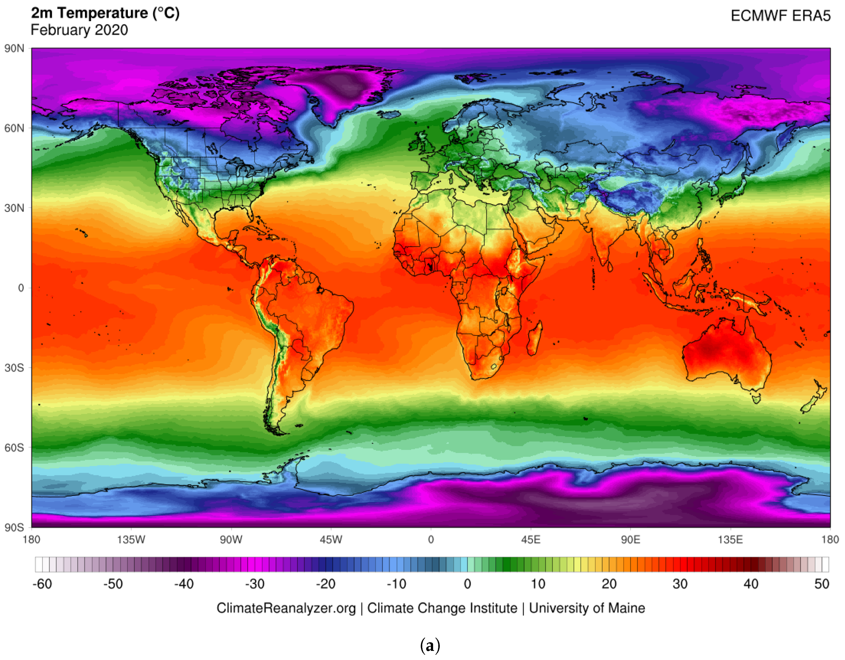
We collected weather data from two different resources [23,24]. For EDA of an earlier stage of the COVID-19 outbreak, we collected average heat maps of air temperature for the entire globe for February and March 2020 from Climate Reanalyzer [23]. Climate Reanalyzer is a project governed by the University of Maine, USA, and it is supported by the National Science Foundation (NSF). Furthermore, we collected average air temperature and RH readings per day for capital cities of the locations considered in this study from a website [24] through web scraping. Although the readings of weather parameters between cities in a country varied greatly, similar to [25], we considered average temperature and RH for capital cities as a reference.

Apart from epidemiological and weather-related data, we also collected data for some other variables, described in

Table 2. List of independent variables used in multiple regression analysis and their descriptions.

No.	Variable	Description
1	Total cases (TC)	Total cases of COVID-19 in each location.
2	Total deaths (TD)	Total deaths due to COVID-19 in each location.
3	TC/million	Ratio of TC and population of the location in millions.
4	TD/million	Ratio of the TD and population of a location in millions.
5	Population	Total population of a location.
6	Population density	Ratio of total population and area of a location.
7	Median age	The median age of the people in a location.
8	Aged 65 or older	Proportion of population 65 years old or older in a location.
9	Aged 70 or older	Proportion of population 70 years old or older in a location.
10	GDP/capita	Gross domestic product per capita which is the measure of a country’s economic output.
11	Cardiovascular death rate	Mortality rate of cardiovascular disease in a location.
12	Diabetes prevalence	The proportion of the population with diabetes.
13	Female smokers	The proportion of females who smoke in a location.
14	Male smokers	The proportion of males who smoke in a location.
15	Hospital beds/thousand	Ratio of total hospital beds to the population of a location in thousands.
16	Life expectancy	The average life expectancy in years for a person in a location.
17	Human development index	A statistic composite index of life expectancy, education, and per capita income of a location.
18	Average temperature	Average of air temperature in °C for the past 7 days experienced in capital city of a location.
19	Average relative humidity (RH)	Average of RH in % for the past 7 days in capital city of a location.

, which include population, population density, median age, those aged 65 and older, those aged 70 and older, gross domestic product (GDP) per capita, cardiovascular death rate, diabetes prevalence, female smokers, male smokers, hospital beds per thousand, life expectancy, and human development index. These variables are constant for each location, as evident from Figure 1, but vary for different locations. Therefore, they can only be used for conducting statistical analysis at a global level by concatenating the data instances of all the locations. These variables were considered in order to further analyze the impact of temperature on the pandemic by taking into account the effect of such important factors. The data related to these variables were collected from Our World in Data [20]. Furthermore, we also fetched the data related to the measures taken in the locations for reducing the spread of the COVID-19 pandemic from official websites of the different locations. The dates at which the selected locations called for a lockdown were fetched from [26].

By using the above mentioned resources, we collected data for nineteen different independent variables, as listed in Table 2, and two dependent or response variables which included NC and ND of COVID-19. After collection of the data, we created a single comma separated (CSV) file, as shown in Figure 1, by concatenating all the variables considered in this study. The CSV file was then processed by using Python [27] for EDA and LR analysis.

3. COVID-19 Outbreak Analysis

The very first case of COVID-19 was reported during December 2019 in China [1]. Initially, it was expected that the neighboring countries of China may become new epicenters of COVID-19. However, the trend manifested a different behavior. The new epicenters were geographically distant from China yet they shared some similarities, as evident from the heat maps of average temperature shown in Figure 2a and Figure 3a. During February 2020, most of China experienced temperatures in the range from 5–15 °C, as shown by green shading in Figure 2a. To some extent, most of China experienced similar temperatures during March 2020, as evident from Figure 3a. Geographically close to China, only South Korea and Japan were affected at the initial stage of the COVID-19 outbreak, and these locations experienced temperatures similar to China, as evident from Figure 2a and Figure 3a. Although many outbound flights were from China to Thailand before the lockdown of Wuhan [28], it was not among the highly affected locations during the earlier stage of the outbreak. Thailand experienced comparatively higher temperatures, as shown by orange shading (>20 °C) in Figure 2a and Figure 3a. This suggests that higher temperatures might have reduced the spread rate of COVID-19 during the initial stage of its outbreak in certain locations.

In order to further explore the trend of the COVID-19 outbreak during its earlier stage, we examined the collected data by defining five different stages, as listed in Table 1. Each stage is discussed further in the following sections.

3.1. Stage I

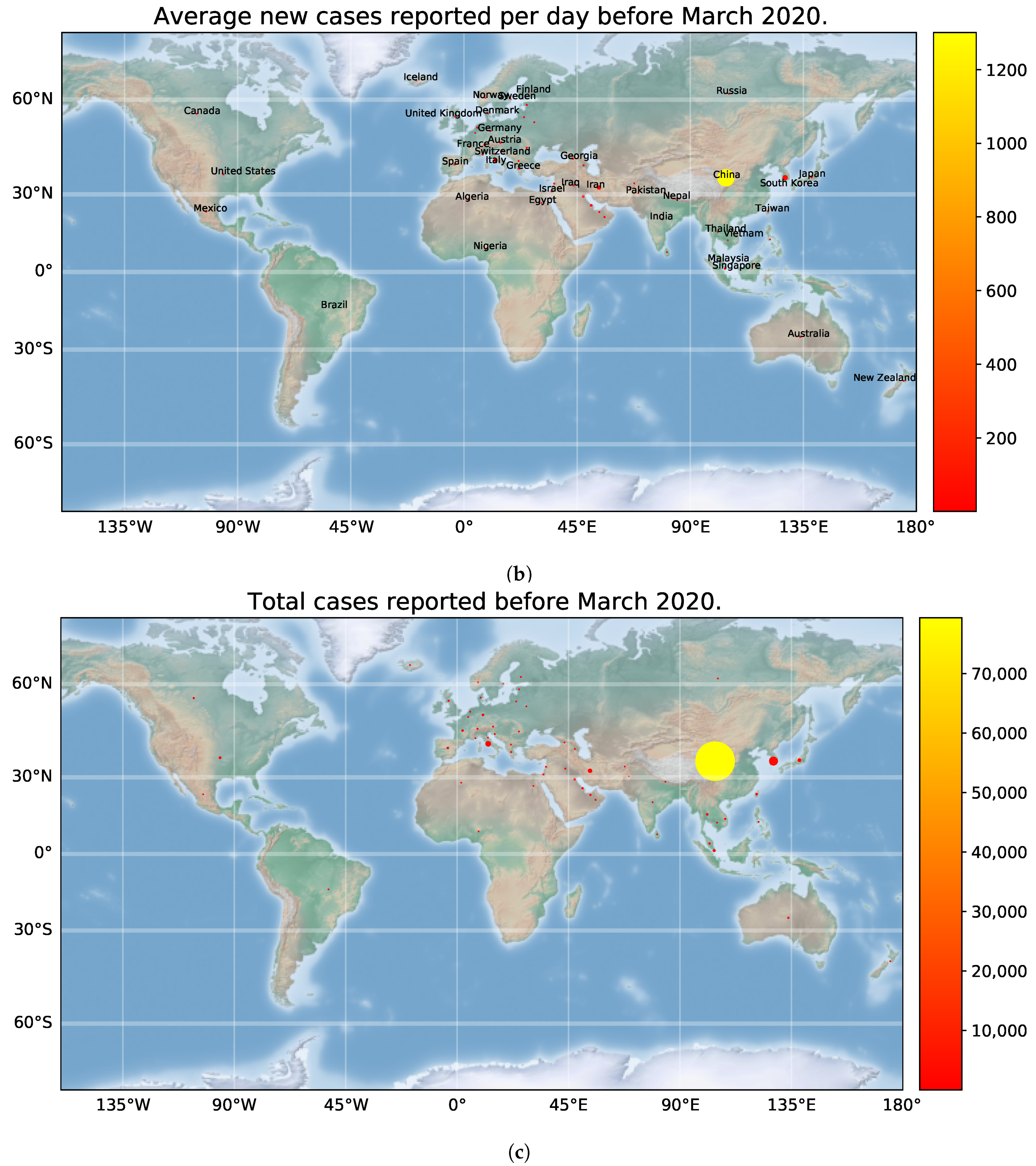
In Stage I, we conducted spatial and temporal pattern analysis of the severity level of the COVID-19 pandemic. By spatial, we mean that we conducted this analysis by considering various locations e.g., France, Australia, and Pakistan, among others. By temporal, we mean that we conducted this analysis by using two different periods, that is, before March 2020 and March 2020. To understand the COVID-19 outbreak during its earlier stage (January–March 2020), we divided the collected epidemiological data into two segments. Since most of the locations experienced the disease during March 2020, the first segment includes all the records before March 2020, and the second includes all the records from 1–26 March 2020. Figure 2b and Figure 3b depict the average number of NC reported in different locations per day. For visual clarity, we did not annotate all the locations. Figure 2c and Figure 3c depict the number of TC reported in different locations by the end of the mentioned period.

After a careful analysis of Figure 2 and Figure 3, it is interesting to note that all the regions with temperatures shown by green shading (5–15 °C) were hit by the pandemic at a higher rate as compared to other regions. All the new epicenters (see Figure 3b,c) experienced almost the same average temperatures. Moreover, the regions of the globe highly affected by this virus during its earlier stage were between the Tropic of Cancer (23.5° N) and the Arctic Circle (67.5° N). In regions below the Tropic of Cancer, the average temperature was higher, and the disease spread at a slower rate. Thailand and Singapore are good examples to consider in support of this pattern [28]. As it is clear from Figure 2b and Figure 3b, the average number of NC reported per day in these regions was small as compared to the regions above the Tropic of Cancer. Furthermore, the regions around and above the Arctic Circle experienced lower temperatures, as shown with blue shading (<0 °C), and the average number of NC reported per day in these regions was also small.

This pattern suggests that at either higher or lower temperatures, the disease spread at a slower rate. Furthermore, in a few published studies [10,29], it has been found that the spread rate of the pandemic was positively correlated with the population density of locations. Therefore, besides lower temperature in regions around the Arctic Circle, another possible reason for slower transmission of the virus could be their low population density.

3.2. Stage II

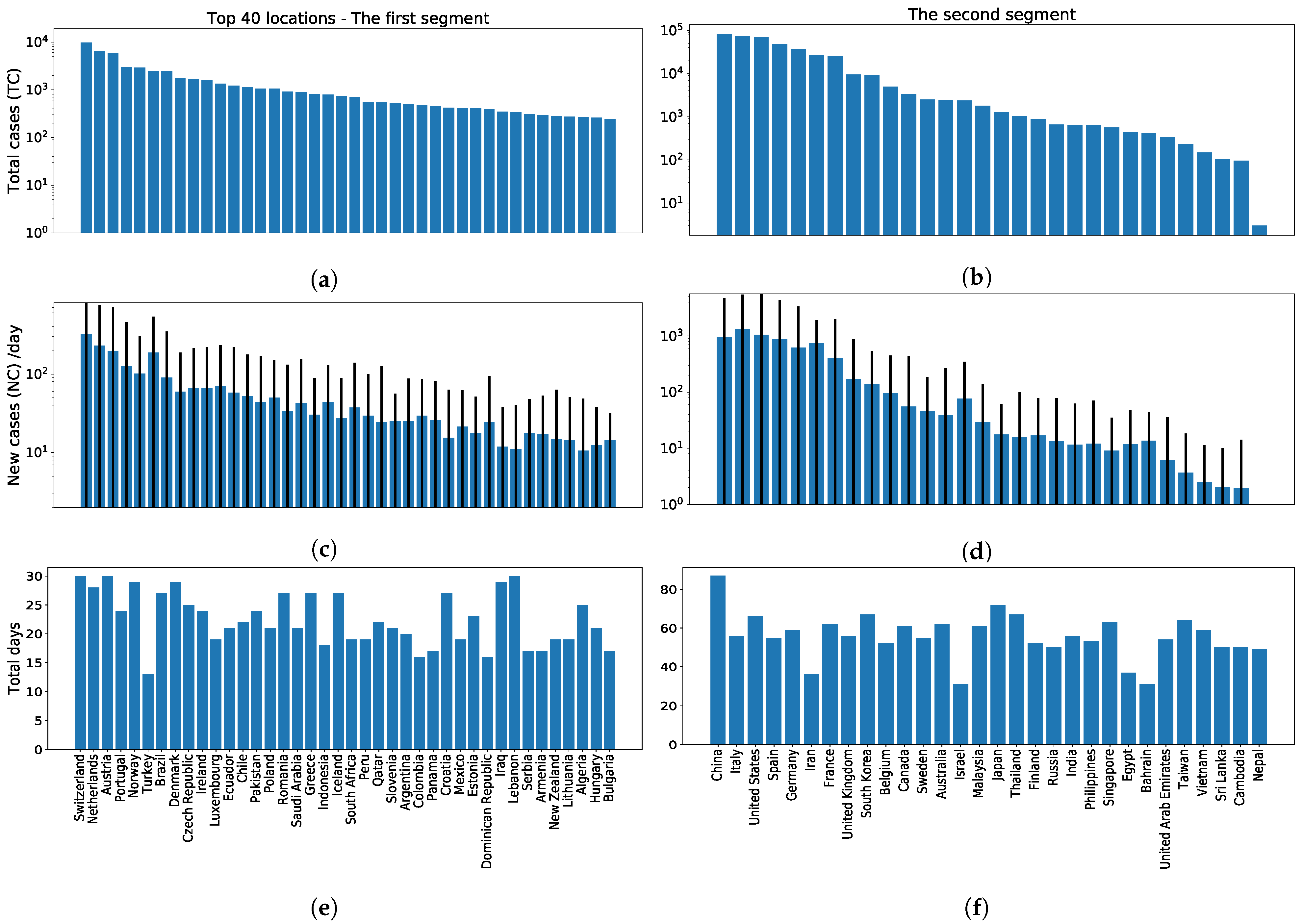
In Stage II, we examined the patterns of TC, mean of NC reported per day, and the number of days since the very first case reported per location. In order to examine these patterns, the epidemiological data were collected for approximately a three-month period, that is, from January to March 2020. Since most of the locations were hit by the pandemic during March, as it is clear from Figure 3b, we divided the collected data into two segments, as depicted by the patterns reported in Figure 4. The first segment includes the locations having a maximum of 30 records and the second segment includes the locations with more than 30 records within the mentioned period of time. According to the collected epidemiological data, most of the locations fell in the first segment since they recorded fewer than 30 records. Therefore, Figure 4a,c,e show the results for the top 40 locations with the largest number of TC. Only a few locations fell in the second segment since they recorded more than 30 records during the initial stage of the outbreak (as shown in Figure 4b,d,f).

Figure 4a,b depict the number of TC reported in each location on 26 March 2020, while Figure 4c,d show the mean of NC reported per day in each location. Note that the vertical lines are used to denote twice of the standard deviations around the mean. In Figure 4e,f, we report the number of days since the first case was reported in each location. The locations along the horizontal axis in Figure 4 are sorted in descending order as a function of TC. Thus, in Figure 4, the locations listed on the left and right side of each plot recorded the larger and smaller numbers of TC, respectively.

A few locations, including Turkey, reported their first case during March 2020. Although the total number of days is small for these locations (see Figure 4e), the growth rate of the virus is quite fast as it is clear from TC reported in Figure 4a. It is interesting to note from Figure 4a that a month after the first COVID-19 case was reported in Switzerland, the Netherlands, Austria, and Portugal, the number of TC exceeded 3000 in each of these locations. However, for Nepal, Sri Lanka, United Arab Emirates, and Taiwan, among others, the number of TC did not exceed 1000 (see Figure 4b). Moreover, the mean of NC reported per day for each of these locations was in the order of tens during the earlier stage of the outbreak, as evident from Figure 4d. However, for the Netherlands, Switzerland, and Portugal, the same value was in the order of hundreds (see Figure 4c).

From the results reported in Figure 4, it is evident that in some locations, the virus had spread at a faster rate compared to others. For example, although the total number of days for Sri Lanka, Cambodia, Nepal, the Philippines, Finland, Italy, and Spain is approximately the same, the number of TC reported in Italy and Spain is in the order of thousands. However, for the rest of the mentioned locations, the number of TC is in the order of hundreds. Similarly, the total number of days for Iran is small although the number of TC is in the order of thousands.

3.3. Stage III

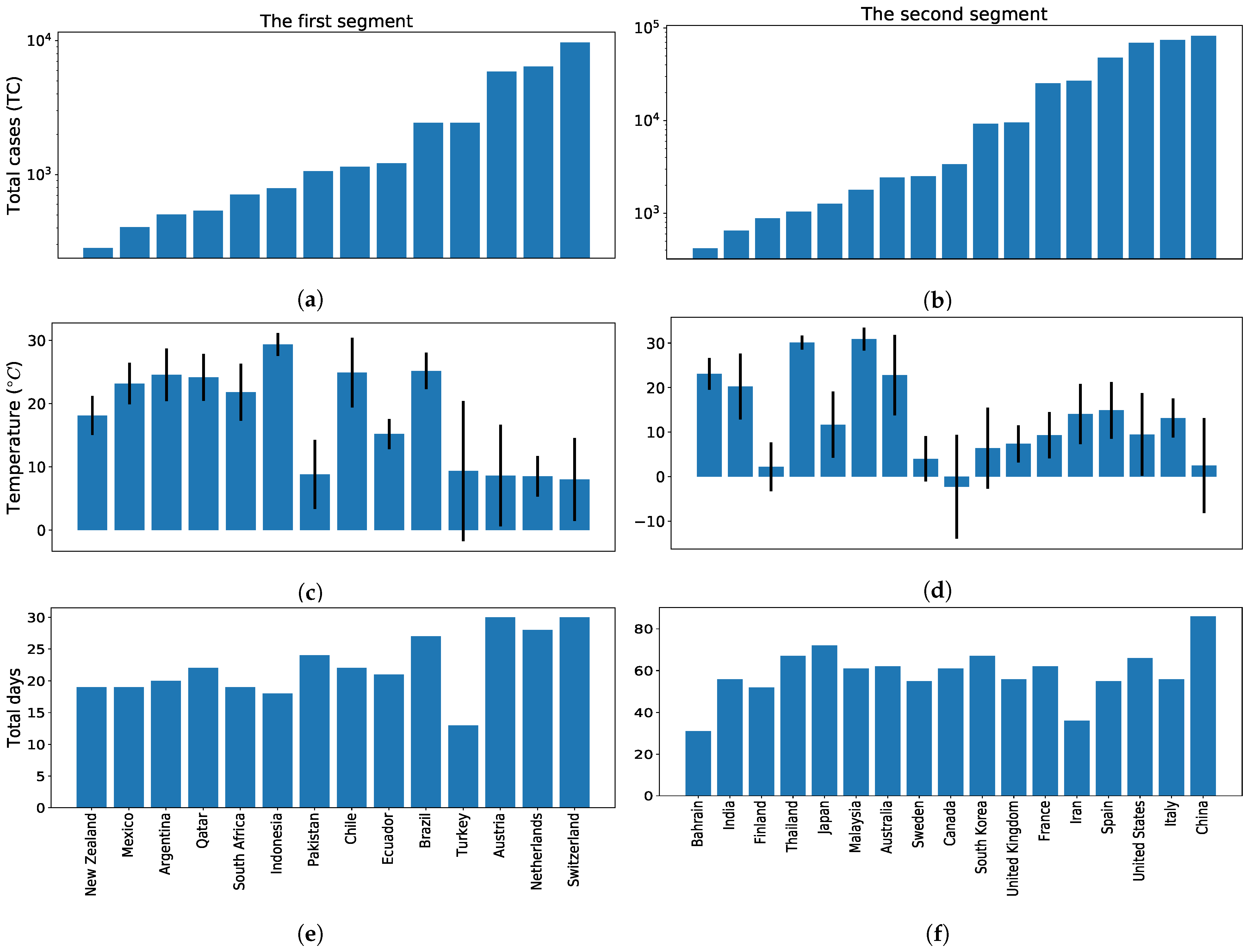
In Stage III, we investigated the pattern of TC, mean of the temperature reported per day, and the number of days since the very first case reported per location. For conducting this analysis, we selected a few locations from around the globe. Moreover, for visual clarity, by following a similar procedure to that described in Stage II, we divided the data for selected locations into two segments, as evident from Figure 5. In the first segment, the locations having records for fewer than 30 days are grouped together. In the second segment, the locations having records for more than 30 days are grouped together.

In Figure 5a,b, we report the number of TC for selected locations. In Figure 5c,d, we report the mean of the temperature reported per day in each location. Furthermore, the vertical lines are used to denote twice of the standard deviation around the mean. Figure 5e,f show the number of days since the very first case reported in each location during the considered period.

After comparing Figure 5a,c, it is evident that the locations with a larger number of TC, which include Switzerland, the Netherlands, Austria, and Turkey, all experienced temperatures with a mean around 10 °C. A similar pattern is evident from Figure 5b,d for China, Italy, the United States, Spain, Iran, France, the United Kingdom, and South Korea. These reported a larger number of TC and experienced temperatures with a mean around 10 °C. Furthermore, a few locations with very low temperatures i.e., Canada, Sweden, and Finland, reported a smaller number of TC. Although the temperatures of Japan, Iran, Italy, and Spain were almost in the same range, Japan reported significantly fewer accumulated cases. According to one of the published reports [30], the use of masks in Japan is very common which could be a reason for the slower growth of the disease in this region.

3.4. Stage IV

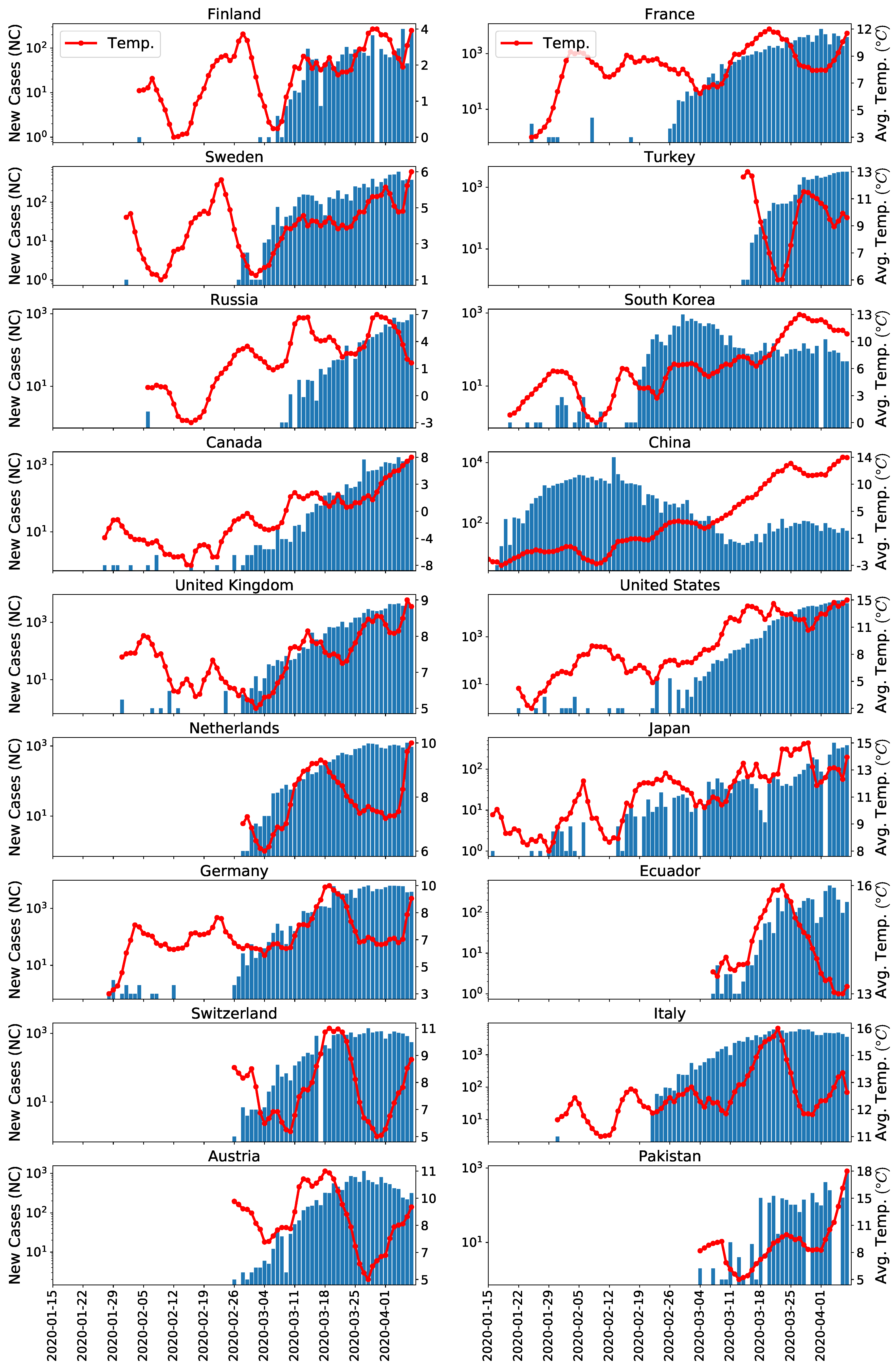
In Stage IV, we analyzed the trends of NC reported per day and average temperature for the past 7 days, for selected locations, by bearing in mind the measures taken in the locations to contain the virus. The trends are depicted in Figure 6 and Figure 7 separately for each location wherein the bar plot denotes the number of NC reported per day and the line plot denotes the average temperature for the past 7 days. It should be noted that the locations in Figure 6 and Figure 7 are organized in ascending order according to the maximum average temperature. For example, the maximum average temperature for Finland was around 4 °C and, for Sweden, it was around 6 °C. Starting from Russia in Figure 6 up to Spain in Figure 7, excluding Japan and Ecuador, the rest of the locations reported more than 1000 NC per day. On the other hand, excluding Brazil, the locations before Russia in Figure 6 and after Spain in Figure 7 reported fewer than 1000 NC per day. Thus, the pattern is suggesting that the rate of spread of the virus was slower in the regions that experienced either higher or lower temperatures. Furthermore, since the locations around the globe opted for different measures in order to reduce the spread of COVID-19, a clear relationship between average temperature and NC reported per day may not be evident from Figure 6 and Figure 7.

During an earlier stage of the COVID-19 outbreak, most of the locations either took necessary measures or opted for a lockdown to reduce the spread of the virus. However, the extent of the lockdown varied between local regions of a location and between different locations. For example, South Korea and Singapore, although being hit at an earlier stage of the outbreak, did not call for a complete lockdown. Instead, they followed a different approach based on testing, tracking, and isolation. Furthermore, both locations are densely populated, were hit by the disease at an earlier stage, and took mostly similar measures to reduce the spread of disease. In the considered scenario, they mainly differed in weather conditions i.e., the average temperature in Singapore was higher as compared to South Korea. Both the locations successfully kept the rate of the spread of the virus under control, as evident from Figure 6 and Figure 7. However, the maximum number of NC reported per day for Singapore was smaller than South Korea. This implies that the variations in regional temperatures might have played a role in the rate of spread of the virus during the initial stage of the outbreak.

Japan reported a smaller number of NC during the earlier stage of the outbreak because the population routinely makes use of masks which reduced the rate of the spread of the virus. Furthermore, New Zealand reported its first case during the first week of March 2020, and experienced temperatures above 20 °C, as evident from Figure 6. However, New Zealand called for a lockdown at an earlier stage of the outbreak, on 25 March 2020, by predicting the rapid growth of the virus in the region. This explains why the rate of spread of the disease came under control in New Zealand. Moreover, the trends of Argentina and South Africa (see Figure 7) are also similar to that of New Zealand (see Figure 6) since South Africa and Argentina also called for a lockdown at an earlier stage of the outbreak, i.e., around 20 March 2020. Although Chile and Brazil also reported their first case in the same period as South Africa and Argentina, the NC reported per day started increasing in these locations since proper measures were not put in place at an earlier stage of the outbreak.

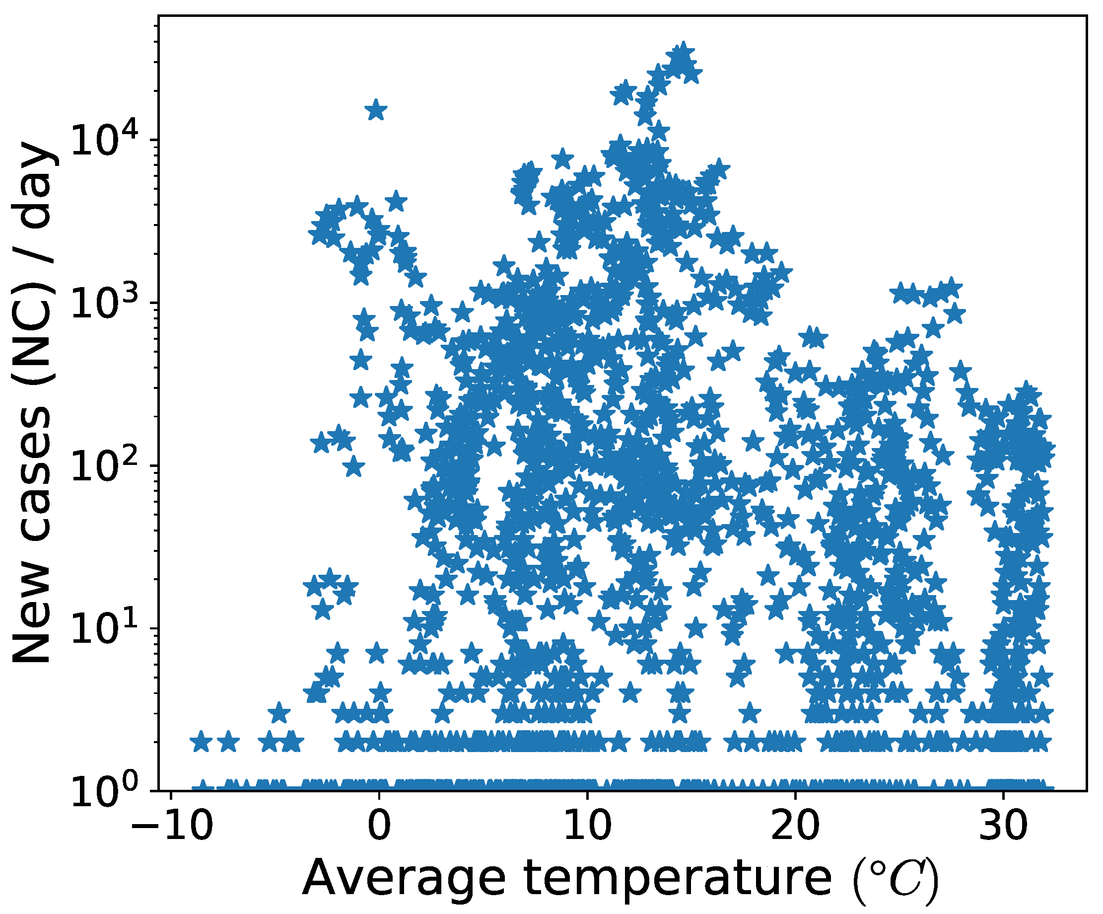
After observing the reported trends for 34 different locations, it can be said that the variations in regional temperatures affected the rate of the spread of the COVID-19 pandemic during the earlier stage of the outbreak. However, due to different measures taken in the locations in order to reduce the spread of the pandemic, the patterns observed for each location differ. This could be a reason behind the contradicting findings reported in the existing literature regarding the impact of temperature on the spread rate of the pandemic [4]. Therefore, for further clarity, in Figure 8, we present the scatter plot of NC reported per day in each location against the average temperature. It is evident from Figure 8 that some of the locations experiencing average temperatures in the moderate range (5–20 °C) reported more than 10,000 NC per day. On the other hand, most of the locations with average temperatures above 20 °C or below 5 °C reported fewer than 1000 NC per day. Hence, there is a consistency in the results reported in this section, that is, the locations experiencing temperatures in the moderate range reported, on average, a larger number of cases.

3.5. Stage V

In Stage V, we analyzed two different patterns for the mortality rate of COVID-19 for the selected locations considered in Stage IV. The first pattern was obtained by taking the ratio of TD and TC reported by each location and the results are depicted in Figure 9a. This pattern gives insight into the mortality rate of COVID-19 in each location. The second pattern was obtained by taking the ratio of TD per location to TD reported around the globe, and the results are depicted in Figure 9b. This pattern gives a global view of mortality due to the pandemic. Figure 9a,b show the two patterns for selected locations for March and April 2020. Since most of the locations called for a lockdown during the third and fourth week of March 2020, it was important to analyze the mortality patterns after two to three weeks of the lockdown.

In order to analyze the patterns of mortality rate as a function of average temperature experienced per location, the horizontal axis in Figure 9 is sorted in ascending order according to the maximum average temperature reported per location. This implies that Finland and Malaysia experienced the smallest and largest maximum average temperatures during the considered period of time, respectively. It is interesting to note from Figure 9a,b that the locations with maximum and minimum average temperatures reported lower mortality rates.

For almost all the locations in Figure 9a, other than China, Iran, Japan, and Bahrain, the mortality rates were high during the first week of April 2020 as compared to the month of March 2020. The locations with mortality rates above 10% during April include Sweden, the United Kingdom, the Netherlands, France, Italy, and Spain. If we look at the global pattern depicted in Figure 9, Italy reported the largest number of deaths during March 2020, and the United States reported the largest number of deaths during the first week of April 2020.

4. Statistical Analysis Using Linear Regression

In the preceding section, with the help of EDA, we found that the regional temperatures played a role in the spread and mortality rates of COVID-19 during the earlier stage of its outbreak. In order to further verify this observation, we employed regression as a statistical analysis technique which is used in situations wherein the relationship between variables under consideration is not deterministic. This means that there is some random component by which the variables are related.

Linear regression (LR) attempts to identify the relationship between dependent and independent variables by obtaining a linear fit to the data. If it is known that there exists a certain linear relationship among the variables, then we can employ LR techniques to obtain a linear fit to the data. By using a dependent variable Y and an independent variable X, the simple linear model is given as

$$Y={\beta }_o+{\beta }_{1}X+ϵ,$$

(1)

where $X,Y,ϵ$ are column vectors, ${\beta }_1$ denotes the slope, ${\beta }_o$ denotes the intercept of the line, and $ϵ$ denotes a random error. If the relationship between dependent and independent variables is exact, then $ϵ=0$ and the above equation becomes deterministic. However, if the relationship between dependent and independent variables is not exact, it means there is some randomness and $ϵ\ne 0$. In such situations, with the help of a simple LR model, the dependent variable Y is approximated $\left(\widehat{Y}\right)$ by fitting a line that best describes the given data. According to a simple LR model, the relationship between the dependent $\left(\widehat{Y}\right)$ and the independent variable $\left(X\right)$ can be approximated through a linear equation, as follows:

$$\widehat{Y}={\beta }_o+{\beta }_{1}X,$$

(2)

where coefficients ${\beta }_o$ and ${\beta }_1$ are unknown and need to be estimated with the help of a given dataset such that the residual error between true $\left(Y\right)$ and fitted $\left(\widehat{Y}\right)$ values is minimized.

Assume that we are given a dataset in the form of tuples $(x^i,y^i)$ where the superscript $i\in \{1,2,\dots ,N\}$ represents the ith instance or observation, $x^i$ denotes the value of an independent variable and $y^i$ denotes the true value of the dependent variable. With the help of LR, if we obtain a fitted model ${\widehat{y}}^i={\beta }_o+{\beta }_1{x}^i$ for approximating the true value of dependent variable $y^i$, then the residual error between true and fitted values for the ith instance can be given as

$$e^i=y^i-{\widehat{y}}^i,i=1,2,\dots ,N.$$

(3)

Thus, the unknown coefficients can be obtained, by minimizing the sum of the squares of residuals between true and fitted values, which is also called as sum of squares of the errors (SSE). This minimization procedure for estimating the coefficients is known as the ordinary least square (OLS) method, where the SSE is defined as

$$SSE=\sum _{i=1}^N{\left(e^i\right)}^2.$$

(4)

By differentiating the above equation with respect to coefficients ${\beta }_o,{\beta }_1$ and setting these to zero, we get the following expressions:

$${\beta }_1=\frac{{\sum }_{i=1}^N(x^i-\overline{x})(y^i-\overline{y})}{{\sum }_{i=1}^N{(x^i-\overline{x})}^2},$$

(5)

$${\beta }_o=\frac{{\sum }_{i=1}^N{y}^i-{\beta }_1{\sum }_{i=1}^N{x}^i}{N}=\overline{y}-{\beta }_1\overline{x}.$$

(6)

In order to assess the fitted model’s adequacy, we use $R^2$, also called the coefficient of determination. This quantity measures the proportion of variability captured by the fitted model. It is defined as

$$R^2=1-\frac{SSE}{SST},$$

(7)

$$SST=\sum _{i=1}^N{(y^i-\overline{y})}^2,$$

(8)

where SST is the total corrected sum of squares.

4.1. Simple Linear Regression Models

For examining the relationship between the NC of COVID-19 reported per day and the average temperature for the past 7 days, we initially conducted a simple LR analysis. We considered data instances for 34 different locations and performed LR analysis for each location separately in order to understand the relationship between the variables under consideration based on the local context. Furthermore, we also performed LR analysis by concatenating all the data instances of locations considered in this study in order to examine the relationship between variables at a global scale.

We obtained simple LR models by using NC as a dependent variable and the average temperature for the past 7 days as an independent variable. Therefore, given data instances in the form of a tuple $(T_r,N{C}_r)$ for location $r\in \{Argentina,Australia,Austria,\dots ,UnitedStates\}$, the simple LR model for fitting $\widehat{NC}$ is given as

$${\widehat{NC}}_r={\beta }_{r_o}^c+{\beta }_{r_1}^c{T}_r.$$

(9)

Moreover, we also obtain another LR model by using ND as a dependent variable and the average temperature for the past 7 days as an independent variable. Thus, given data instances in the form of a tuple $(T_r,N{D}_r)$, the simple LR model for fitting $\widehat{ND}$ reported per day is given as

$${\widehat{ND}}_r={\beta }_{r_o}^d+{\beta }_{r_1}^d{T}_r.$$

(10)

Apart from these location-based models, we also obtained one cumulative model by concatenating data instances of all the locations considered in this study.

4.2. Multiple Linear Regression Models

In order to further examine the effect of temperature on the overall spread and mortality rates of COVID-19, we also performed multiple regression analysis by considering nineteen independent variables, as listed in Table 2. We performed this analysis at a global level only, that is, we concatenated all the data instances of the locations considered in this study. Hence, given the dataset in the form of a tuple $(X_1,X_2,\dots ,X_j,\dots ,X_{19},NC)$ where $X_j$ denotes the independent variable and NC is a dependent variable, then the multiple LR model is given as

$$\widehat{NC}={\beta }_o^c+{\beta }_1^c{X}_1+{\beta }_2^c{X}_2,\dots ,{\beta }_{19}^c{X}_{19}.$$

(11)

Similarly, given the dataset in the form of a tuple $(X_1,X_2,\dots ,X_{19},ND)$ where ND is a dependent variable, then the multiple LR model is given as

$$\widehat{ND}={\beta }_o^d+{\beta }_1^d{X}_1+{\beta }_2^d{X}_2,\dots ,{\beta }_{19}^d{X}_{19}.$$

(12)

4.3. F-Test Statistic

We employed the F-test statistic for checking the significance of the conducted regression analysis. The F-test statistic indicates whether the LR model provides a better fit to the data than a model that contains no independent variables. It is used to test the null hypothesis against an alternate hypothesis, as defined below:

$$\begin{array}{cc}\hfill H_o:& {\beta }_1={\beta }_2={\beta }_3=\dots {\beta }_k=0,\hfill \\ \hfill H_1:& {\beta }_j\ne 0.\hfill \end{array}$$

(13)

Here, the null hypothesis $\left(H_o\right)$ suggests that there is no relation between dependent and independent variables since the coefficients are zero. The alternate hypothesis $\left(H_1\right)$ suggests that there is a relationship between the dependent variable and at least one independent variable. The F-test statistic is defined as

$$F=\frac{SSR/k}{SSE/(N-k-1)},$$

(14)

$$SSR=\sum _{i=1}^N{({\widehat{y}}^i-\overline{y})}^2,$$

(15)

here, k denotes the total number of independent variables, and SSR stands for the sum of squares regression.

In null hypothesis significance testing, the p-value denotes the lowest level of significance at which the observed value of a test is significant. If the p-value obtained through the F-test statistic is smaller than the defined significance level $\alpha$, then the null hypothesis is rejected. Generally, $\alpha$ is set to the 0.05 level which implies a 95% confidence level.

4.4. t-Test Statistic

In the case of multiple LR analysis, we also employed a t-test which is used to check the significance of individual regression coefficients. The t-test statistic for the jth independent variable can be obtained as

$$t=\frac{{\widehat{\beta }}_j}{SE\left({\beta }_j\right)},$$

(16)

where SE is the standard error. If the p-value obtained through the t-test statistic for the jth coefficient is less than the defined significance level $\alpha$, it implies that the jth independent variable significantly contributes in the multiple regression model.

5. Results and Discussion

All the results reported in this section were obtained by using Python [27]. Here, we summarize the insights extracted after performing the EDA in Section 3, and we also discuss the results obtained after performing simple and multiple LR analysis defined in Section 4.1 and Section 4.2, respectively. For clarity and readability, the results of each conducted analysis are discussed separately in the following subsections. Moreover, for further verification, we also performed some additional experiments by assuming different time scales, and the details can be found in the Supplementary Materials.

5.1. Data Analysis Findings

The insights extracted after conducting a detailed EDA of an earlier stage of the COVID-19 outbreak, in Section 3, are summarized as follows.

• The spread and mortality rates of COVID-19 were slower in the regions experiencing extreme temperatures, that is, greater than 20 °C or less than 5 °C.
• Due to different policies adopted by locations around the globe in order to contain the spread of the pandemic, a clear relationship between temperature and the spread or mortality rates of COVID-19 may not be observable.
• As opposed to other locations, instead of a lockdown, South Korea and Singapore opted for a different strategy based on testing, tracking, and isolation. As a result, compared to other locations, they reported a smaller number of COVID-19 cases. However, as compared to South Korea, Singapore reported a smaller number of cases. It should be noted that the average temperature in Singapore during the earliest stage of the COVID-19 outbreak was high compared to South Korea.
• Although Spain, Italy, Japan, and Iran experienced temperatures almost in the same range, Japan reported a considerably smaller number of COVID-19 cases. According to a published report [30], the use of masks is common in Japan. That is why the spread of pandemic in Japan was comparatively slower.
• New Zealand took strict measures during the earliest stage of the outbreak. Although New Zealand experienced temperatures in a range similar to Spain, Iran, and Italy, it reported a very small number of COVID-19 cases.

From the above insights, it is evident that temperature impacted the spread rate of COVID-19 during its earlier stage. However, these insights were extracted by analyzing data from January to March 2020. Due to different seasons, the weather conditions of a location change during the year. Therefore, in order to further investigate the impact of temperature on the spread and mortality rates of the COVID-19 pandemic, in the following sections, we discuss the results obtained after applying statistical analysis by using data for one complete year (2020).

5.2. Simple Linear Regression Analysis

In this section, we report the results obtained after performing simple LR analysis discussed in Section 4.1. For each location, two simple linear models were obtained after applying (9) and (10), that is, one for fitting the NC and another for fitting the ND reported per day. Moreover, the temperature average for the past 7 days was used as an independent variable in order to approximate the value for dependent variables NC or ND. In

Table 3. Results of simple LR analysis by using new cases (NC) or new deaths (ND) of COVID-19 per day and average temperature as a dependent and independent variable, respectively. For further analysis, the temperature mean and standard deviation experienced in each location are also mentioned. The number of total cases (TC) and total deaths (TD) per one million recorded in each location by the end of December 2020 is also reported.

Location (r)	(TC,TD) in Millions	Temp.(°C) $({\mathit{\mu }}_{\mathit{r}},{\mathit{\sigma }}_{\mathit{r}})$	$\widehat{\mathit{NC}}={\mathit{\beta }}_{{\mathit{r}}_{\mathit{o}}}^{\mathit{c}}+{\mathit{\beta }}_{{\mathit{r}}_1}^{\mathit{c}}{\mathit{T}}_{\mathit{r}}$		$\widehat{\mathit{ND}}={\mathit{\beta }}_{{\mathit{r}}_{\mathit{o}}}^{\mathit{d}}+{\mathit{\beta }}_{{\mathit{r}}_1}^{\mathit{d}}{\mathit{T}}_{\mathit{r}}$
			$({\mathit{\beta }}_{{\mathit{r}}_{\mathit{o}}}^{\mathit{c}},{\mathit{\beta }}_{{\mathit{r}}_1}^{\mathit{c}})$	p-Value	$({\mathit{\beta }}_{{\mathit{r}}_{\mathit{o}}}^{\mathit{d}},{\mathit{\beta }}_{{\mathit{r}}_1}^{\mathit{d}})$	p-Value
Finland	(0.034,0.0005)	(10.39,7.36)	(198,−9.03)	0.00	(2.2,−0.11)	0.00
Russia	(3.02,0.054)	(10.86,9.02)	(13,720,−393)	0.00	(248,−7)	0.00
Canada	(0.54,0.015)	(11.68,11.19)	(2499,−75.87)	0.00	(46,−0.693)	0.007
Sweden	(0.396,0.008)	(11.7,6.88)	(2377,−96.9)	0.0004	(34.2,−1.17)	0.00
United Kingdom	(2.26,0.0705)	(11.95,4.16)	(18,260,−942)	0.00	(407,−20)	0.00
Ecuador	(0.21,0.014)	(13.86,2.58)	(1067,−27.97)	0.242	(71.35,−1.69)	0.82
Germany	(1.65,0.0303)	(14.17,7.33)	(13,900,−620)	0.00	(261,−12.61)	0.00
Switzerland	(0.428,0.007)	(14.23,7.5)	(4022,−178.4)	0.00	(73.15,−3.58)	0.00
New Zealand	(0.002,0.00003)	(14.38,2.79)	(−12.5,1.32)	0.002	(0.042,−0.0012)	0.801
Netherlands	(0.774,0.011)	(14.55,5.83)	(7191,−310.3)	0.00	(86.5,−3.9)	0.00
Austria	(0.351,0.0059)	(15.06,7.79)	(3446,−147)	0.00	(72.4,−3.5)	0.00
Australia	(0.028,0.0009)	(15.12,5.86)	(239,−10)	0.036	(9.26,−0.43)	0.00
France	(2.616,0.063)	(15.38,6.61)	(14,660,−440)	0.0009	(412,−16.7)	0.00
China	(0.095,0.0048)	(15.68,10.94)	(845,−35.1)	0.00	(31.3,−1.30)	0.00
South Korea	(0.057,0.0008)	(16.28,9.25)	(420,−14.7)	0.00	(5.73,−0.2)	0.00
South Africa	(1.00,0.0267)	(17.9,3.41)	(8310,−261)	0.0012	(227,−7.3)	0.0001
Argentina	(1.57,0.0425)	(18.05,4.99)	(7647,−106.3)	0.097	(157,−0.18)	0.95
Chile	(0.598,0.0164)	(18.13,5.79)	(5389,−183.5)	0.00	(181,−6.8)	0.00
Turkey	(2.147, 0.0198)	(18.29,8.51)	(30,620,−1254)	0.0012	(169,−5.7)	0.00
United States	(18.98,0.332)	(18.6,8.33)	(91,530,−1811)	0.00	(1022,−7.26)	0.170
Japan	(0.221,0.0031)	(19.48,7.22)	(1111.5,−23)	0.0009	(16,−0.38)	0.00
Spain	(1.854,0.0498)	(20.55,8.07)	(10,430,−226)	0.0008	(381.7,−0.2)	0.00
Mexico	(1.377,0.122)	(20.88,2.3)	(26,900,−1055)	0.00	(1605,−56.2)	0.00
Italy	(2.038,0.716)	(21.49,7.51)	(17,400,−512)	0.00	(629,−20.1)	0.00
Pakistan	(0.471,0.0098)	(22.45,11.14)	(538,48)	0.00	(14.18,0.87)	0.0008
Iran	(1.20,0.0547)	(22.64,9.6)	(8281,−188)	0.00	(257,−3.36)	0.00
Brazil	(7.465,0.19)	(25.16,2.41)	(54,730,−1130)	0.035	(2334,−66.6)	0.00
India	(10.21,0.148)	(26.81,6.76)	(−7189,1493)	0.00	(27.2,−255.6)	0.00
Singapore	(0.058,0.00003)	(29.31,3.28)	(−181,10.9)	0.0009	(−0.12,0.0064)	0.139
Thailand	(0.006,0.00006)	(29.44,3.67)	(3.28,0.47)	0.597	(−0.298,0.014)	0.044
Malaysia	(0.105,0.00045)	(29.66,2.98)	(302,0.85)	0.927	(−0.24,0.05)	0.174
Indonesia	(0.713, 0.0212)	(29.83,0.98)	(23,880,−716)	0.00	(464,−13)	0.004
Bahrain	(0.092,0.00035)	(31.65,6.12)	(−558,27.5)	0.00	(−2.49,0.12)	0.00
Qatar	(0.143,0.00024)	(32.96,6.28)	(−708,35.8)	0.00	(−2.4,0.098)	0.00
Cumulative	NA	NA	(7074,−53.8)	0.011	(132.59,−0.43)	0.169

, ${\beta }_{r_o}^c$ and ${\beta }_{r_1}^c$ denote the bias and coefficient of average temperature, respectively, obtained after applying simple LR for estimating NC in each location. Similarly, ${\beta }_{r_o}^d$ and ${\beta }_{r_1}^d$ denote the bias and coefficient of average temperature, respectively, obtained after applying simple LR for estimating ND in each location.

Apart from location-based simple LR models, at the end of Table 3, we also report a cumulative LR model which was obtained after concatenating the data instances of all the locations considered in this study. Moreover, we report the mean $\left({\mu }_r\right)$ and standard deviation $\left({\sigma }_r\right)$ of the temperature experienced in a location during the mentioned period of time, and the locations in Table 3 are sorted in ascending order according to ${\mu }_r$. Furthermore, we also report in Table 3 the numbers of TC and TD, in millions, reported per location by the end of December 2020. After analyzing the impact of average regional temperatures on NC or ND of COVID-19 from the results given in Table 3, the following insights were extracted.

• Excluding Ecuador, Argentina, Thailand, and Malaysia, the p-value for the rest of the locations is much smaller than the defined significance level $\alpha =0.05$. This implies that the null hypothesis is rejected and the results reveal a significant relationship between NC and average temperature for most of the locations with a 95% confidence level.
• The linear models obtained for a few locations, which include New Zealand, Pakistan, India, Singapore, Bahrain, and Qatar, show a significant positive relationship between average temperature and NC reported per day with a confidence level of 99.9%. This implies that when the average temperature in these locations increases, the number of NC increases. However, excluding India, the rest of the mentioned locations reported a smaller number of TC.
• The linear models obtained for Ecuador, New Zealand, Argentina, the United States, Singapore, and Malaysia depict an insignificant relationship between average temperature and ND reported per day.
• The linear models obtained for Pakistan, Thailand, and Qatar depict a significant positive relationship between average temperature and ND with a confidence level of 95%. This implies that when the average temperature in these location increases, the number of ND increases. However, the number of TD is much smaller in the mentioned locations.
• It is evident from Table 3 that the locations showing an insignificant relationship between average temperature and NC or ND experienced temperatures with a standard deviation ${\sigma }_r$ of less than 5 °C.
• Other than Singapore, the locations showing a significant positive relationship between average temperature and NC or ND experienced temperatures with mean ${\mu }_r>22$ °C and standard deviation ${\sigma }_r>6$ °C. Although the mentioned locations experienced temperatures in a higher range and showed a positive relationship with NC or ND, excluding India, the rest of the locations reported a smaller number of TC. For example, Thailand, Malaysia, Qatar, Bahrain, and Singapore reported a smaller number of COVID-19 cases.

It is evident from the reported results that, for most of the locations, a significant inverse relationship has been observed between NC or ND and average temperature. Although some locations have shown a significant positive relationship between average temperature and NC or ND, most of them reported a smaller number of total COVID-19 cases and deaths. Moreover, the cumulative model developed for fitting NC revealed a significant inverse relationship with average temperature. However, the cumulative model developed for fitting ND has not revealed a significant relationship with average temperature since its p-value is greater than the defined significance level, that is, $\alpha =0.05$.

5.3. Multiple Linear Regression Analysis

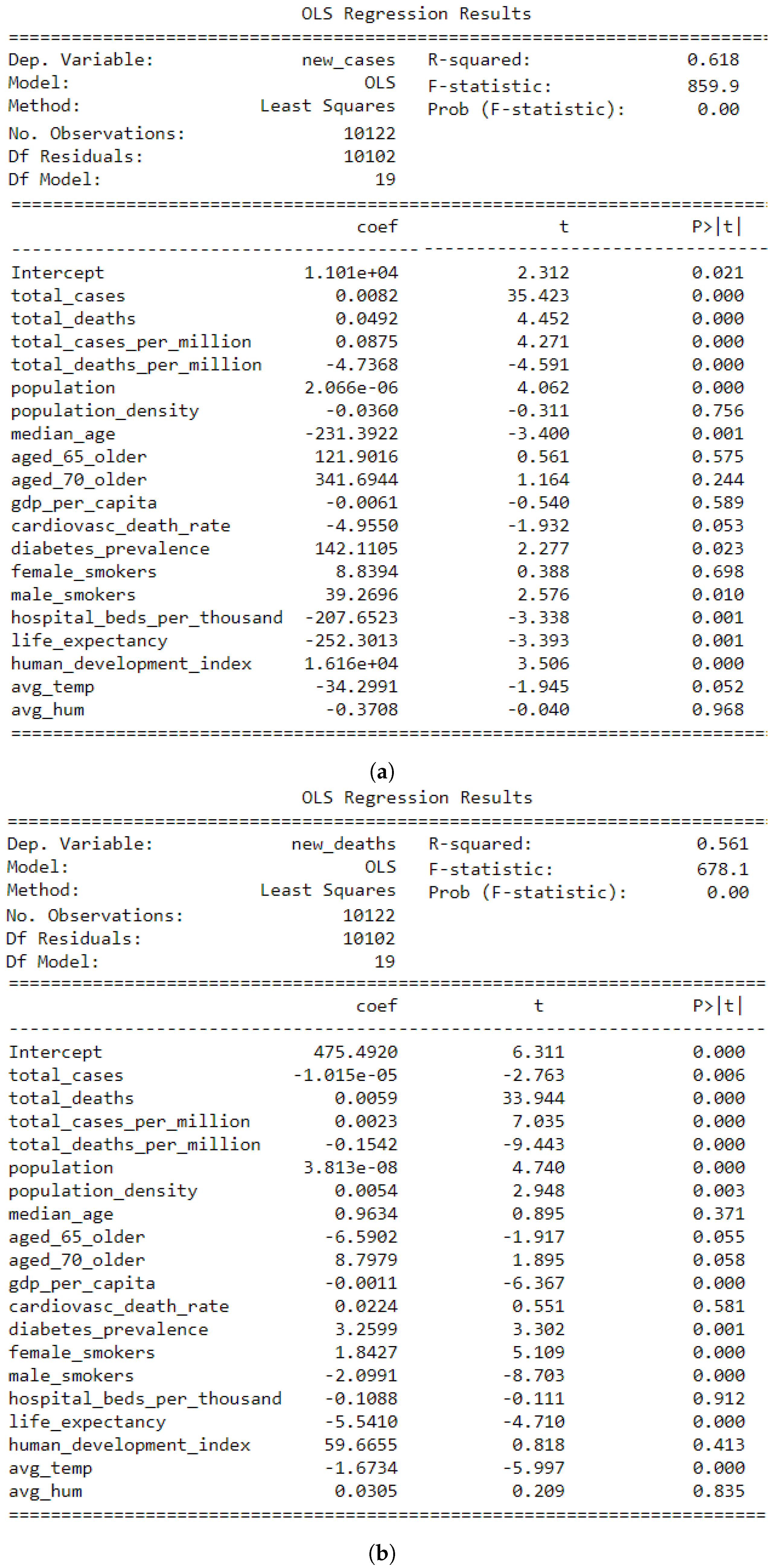
In this section, we report the results obtained after performing the multiple LR analysis discussed in Section 4.2. By using nineteen independent variables defined in Table 2, we obtained two multiple LR models. The first model was obtained for fitting NC by using (11), and its results are reported in Figure 10a. The second model was obtained for fitting ND by using (12), and its results are reported in Figure 10b. The p-value of the F-test statistic, that is, Prob (F-statistic) in Figure 10, provides the overall significance of the developed multiple LR models. Moreover, the p-value of the t-statistic $(p>|t\left|\right)$ provides the significance of each independent variable by considering the rest of the independent variables as constants. The values fitted by the multiple LR models are close to the true values, as evident from Figure 10, since the coefficient of determination $R^2$ is above 0.5. After analyzing the results reported in Figure 10a, the following insights were extracted.

• It is evident from the F-test statistic that the developed multiple LR model is significant since the p-value (Prob (F-statistic) in Figure 10) is approximately zero. This implies that the independent variables considered in this analysis play a significant role in the spread rate of COVID-19.
• The t-test statistic reveals that the variables which significantly affected the NC include TC, TD, TC per million, TD per million, population, human development index, cardiovascular death rate, diabetes prevalence, hospital beds per thousand, life expectancy, and average temperature.
• The variables which have not significantly affected the dependent variable include population density, those aged 65 and older, those aged 70 and older, GDP per capita, female smokers, and average RH.
• The variables TC, TD, TC per million, population, diabetes prevalence, male smokers, and human development index show a significant positive relationship with NC reported per day. This implies that a location with larger values of the mentioned variables will show a larger number of NC.
• The variables TD per million, median age, cardiovascular death rate, hospital beds per thousand, life expectancy, and average temperature show a significant inverse relationship with NC reported per day. This implies that a location with larger values of the mentioned variables will show a smaller number of NC.

From above details, it is evident that even in the presence of multiple other factors, the effect of average temperature is significant on the spread rate of COVID-19.

In order to analyze the impact of average temperature on ND in the presence of other important variables, the results obtained after performing multiple LR analysis using (12) are reported in Figure 10b and discussed below.

• It is evident from the F-test statistic that the developed multiple LR model is significant since the p-value is approximately zero. This implies that the considered variables played a role in overall ND reported per day due to COVID-19.
• The variables which have not significantly affected the dependent variable include median age, those aged 65 and older, those aged 70 and older, cardiovascular death rate, hospital beds per thousand, human development index, and average RH.
• The variables TD, TC per million, population, population density, diabetes prevalence, and female smokers show a significant positive relationship with ND. This implies that a location with larger values of the mentioned variables will show a larger number of ND.
• The variables TC, TD per million, GDP per capita, male smokers, life expectancy, and average temperature show a significant inverse relationship with ND reported per day. This implies that a location with larger values of the mentioned variables will report a smaller number of ND.

From above details, it is evident that even in the presence of multiple other factors, the effect of temperature is significant on the mortality rate of COVID-19.

6. Conclusions

In this work, initially by employing the EDA technique, we examined the impact of regional temperature on spread and mortality rates of the COVID-19 pandemic during an earlier stage of its outbreak. We observed that the spread and mortality rates of COVID-19 were slower in the regions with extreme temperatures. In order to further investigate the impact of regional temperature on the pandemic, we extended the analysis by using simple and multiple LR techniques and using data for one year, that is, from January to December 2020. Under simple LR analysis, for most of the locations, the results revealed a significant inverse relationship between NC or ND reported per day and average temperature. Similarly, the results obtained after conducting multiple LR analysis revealed a significant inverse relationship between average temperature and NC or ND. Although a few locations, which include India, Pakistan, Singapore, Qatar, and Bahrain, experienced high temperatures, the pandemic in these locations showed a significant positive relationship with average temperature. However, excluding India, the rest of the locations reported a smaller number of total COVID-19 cases. Although the pandemic showed an inverse relationship between average temperature and NC or ND in some locations with moderate temperatures (i.e., the United Kingdom, South Africa, Argentina, Ecuador, Chile, Mexico, among others), they reported a larger number of total COVID-19 cases.

Thus, it can be concluded that average temperature has significantly impacted the COVID-19 pandemic, although the exact relationship depends on the range of temperature experienced by a location. That is why some locations have shown a significant positive and others a significant inverse relationship with NC or ND. However, due to different policies adopted in the locations in order to reduce the spread of the pandemic, it is hard to define the range of temperatures wherein a negative relationship is observed between average temperature and NC or ND. Nonetheless, the overall patterns of the pandemic and the results of statistical analysis reveal a significant impact of temperature on the spread and mortality rates of COVID-19.

References

- Harapan, H.; Itoh, N.; Yufika, A.; Winardi, W.; Keam, S.; Te, H.; Megawati, D.; Hayati, Z.; Wagner, A.L.; Mudatsir, M. Coronavirus disease 2019 (COVID-19): A literature review. J. Infect. Public Health 2020. [Google Scholar] [CrossRef] [PubMed]
- World Health Organization. Novel Coronavirus Diesease (2019-nCoV) Pandemic. 2020. Available online: https://www.who.int/emergencies/diseases/novel-coronavirus-2019 (accessed on 23 February 2021).
- Li, Y.; Reeves, R.M.; Wang, X.; Bassat, Q.; Brooks, W.A.; Cohen, C.; Moore, D.P.; Nunes, M.; Rath, B.; Campbell, H.; et al. Global patterns in monthly activity of influenza virus, respiratory syncytial virus, parainfluenza virus, and metapneumovirus: A systematic analysis. Lancet Glob. Health 2019, 7, e1031–e1045. [Google Scholar] [CrossRef] [Green Version]
- Bloom-Feshbach, K.; Alonso, W.J.; Charu, V.; Tamerius, J.; Simonsen, L.; Miller, M.A.; Viboud, C. Latitudinal variations in seasonal activity of influenza and respiratory syncytial virus (RSV): A global comparative review. PLoS ONE 2013, 8, e54445. [Google Scholar]
- Zaitchik, B.F.; Sweijd, N.; Shumake-Guillemot, J.; Morse, A.; Gordon, C.; Marty, A.; Trtanj, J.; Luterbacher, J.; Botai, J.; Behera, S.; et al. A framework for research linking weather, climate and COVID-19. Nat. Commun. 2020, 11, 1–3. [Google Scholar] [CrossRef] [PubMed]
- Briz-Redón, Á.; Serrano-Aroca, Á. The effect of climate on the spread of the COVID-19 pandemic: A review of findings, and statistical and modelling techniques. Prog. Phys. Geogr. Earth Environ. 2020, 44, 591–604. [Google Scholar] [CrossRef]
- Wang, J.; Tang, K.; Feng, K.; Lin, X.; Lv, W.; Chen, K.; Wang, F. Impact of Temperature and Relative Humidity on the Transmission of COVID-19: A Modeling Study in China and the United States. BMJ Open Forthcom. 2021, 11, e043863. [Google Scholar] [CrossRef] [PubMed]
- Poirier, C.; Luo, W.; Majumder, M.S.; Liu, D.; Mandl, K.D.; Mooring, T.A.; Santillana, M. The role of environmental factors on transmission rates of the COVID-19 outbreak: An initial assessment in two spatial scales. Sci. Rep. 2020, 10, 1–11. [Google Scholar] [CrossRef] [PubMed]
- Bherwani, H.; Gupta, A.; Anjum, S.; Anshul, A.; Kumar, R. Exploring dependence of COVID-19 on environmental factors and spread prediction in India. NPJ Clim. Atmos. Sci. 2020, 3, 1–13. [Google Scholar] [CrossRef]
- Jahangiri, M.; Jahangiri, M.; Najafgholipour, M. The sensitivity and specificity analyses of ambient temperature and population size on the transmission rate of the novel coronavirus (COVID-19) in different provinces of Iran. Sci. Total Environ. 2020, 728, 138872. [Google Scholar] [CrossRef] [PubMed]
- Iqbal, N.; Fareed, Z.; Shahzad, F.; He, X.; Shahzad, U.; Lina, M. Nexus between COVID-19, temperature and exchange rate in Wuhan City: New findings from Partial and Multiple Wavelet Coherence. Sci. Total Environ. 2020, 729, 138916. [Google Scholar] [CrossRef] [PubMed]
- Shokouhi, M.; Miralles-Wilhelm, F.; Amoroso, M.A.; Sajadi, M.M. Temperature, Humidity, and Latitude Analysis to Predict Potential Spread and Seasonality for COVID-19. 2020. Available online: https://ssrn.com/abstract=3550308 (accessed on 23 February 2021).
- Sajadi, M.M.; Habibzadeh, P.; Vintzileos, A.; Shokouhi, S.; Miralles-Wilhelm, F.; Amoroso, A. Temperature, humidity, and latitude analysis to estimate potential spread and seasonality of coronavirus disease 2019 (COVID-19). JAMA Netw. Open 2020, 3, e2011834. [Google Scholar] [CrossRef] [PubMed]
- Sobral, M.F.F.; Duarte, G.B.; da Penha Sobral, A.I.G.; Marinho, M.L.M.; de Souza Melo, A. Association between climate variables and global transmission oF SARS-CoV-2. Sci. Total Environ. 2020, 729, 138997. [Google Scholar] [CrossRef] [PubMed]
- Demongeot, J.; Flet-Berliac, Y.; Seligmann, H. Temperature Decreases Spread Parameters of the New COVID-19 Case Dynamics. Biology 2020, 9, 94. [Google Scholar] [CrossRef] [PubMed]
- Ma, Y.; Zhao, Y.; Liu, J.; He, X.; Wang, B.; Fu, S.; Yan, J.; Niu, J.; Zhou, J.; Luo, B. Effects of temperature variation and humidity on the death of COVID-19 in Wuhan, China. Sci. Total Environ. 2020, 724, 138226. [Google Scholar] [CrossRef] [PubMed]
- Coelho, M.T.P.; Rodrigues, J.F.M.; Medina, A.M.; Scalco, P.; Terribile, L.C.; Vilela, B.; Diniz-Filho, J.A.F.; Dobrovolski, R. Global expansion of COVID-19 pandemic is driven by population size and airport connections. PeerJ 2020, 8, e9708. [Google Scholar] [CrossRef]
- Yuan, J.; Wu, Y.; Jing, W.; Liu, J.; Du, M.; Wang, Y.; Liu, M. Non-linear correlation between daily new cases of COVID-19 and meteorological factors in 127 countries. Environ. Res. 2021, 193, 110521. [Google Scholar] [CrossRef] [PubMed]
- Guo, C.; Bo, Y.; Lin, C.; Li, H.B.; Zeng, Y.; Zhang, Y.; Hossain, M.S.; Chan, J.W.; Yeung, D.W.; Kwok, K.O.; et al. Meteorological factors and COVID-19 incidence in 190 countries: An observational study. Sci. Total Environ. 2021, 757, 143783. [Google Scholar] [CrossRef] [PubMed]
- Hannah Ritchie. Coronavirus Source Data. 2020. Available online: https://ourworldindata.org/coronavirus-source-data (accessed on 23 February 2021).
- European Center for Disease Control and Prevention. COVID-19. 2020. Available online: https://www.ecdc.europa.eu/en (accessed on 23 February 2021).
- Dong, E.; Du, H.; Gardner, L. An interactive web-based dashboard to track COVID-19 in real time. Lancet Infect. Dis. 2020, 20, 533–534. [Google Scholar] [CrossRef]
- Climate Change Institute. Climate Reanalyzer. 2020. Available online: https://climatereanalyzer.org/ (accessed on 23 February 2021).
- Time and Data. TimeandData. 2020. Available online: https://www.timeanddate.com/ (accessed on 23 February 2021).
- Jamil, T.; Alam, I.; Gojobori, T.; Duarte, C.M. No evidence for temperature-dependence of the COVID-19 epidemic. Front. Public Health 2020, 8, 436. [Google Scholar] [CrossRef] [PubMed]
- Kaplan, J.; Frias, L.; McFall-Johnsen, M. Coronavirus: How Japan Keeps COVID-19 under Control. 2020. Available online: https://www.businessinsider.com/countries-on-lockdown-coronavirus-italy-2020-3 (accessed on 23 February 2021).
- Van Rossum, G.; Drake, F.L. Python 3 Reference Manual; CreateSpace: Scotts Valley, CA, USA, 2009. [Google Scholar]
- CGTN. Five Million People Left Wuhan before the Lockdown, Where Did They Go? 2020. Available online: https://news.cgtn.com/news/2020-01-27/5-million-people-left-Wuhan-before-the-lockdown-where-did-they-go–NACCu9wItW/index.html (accessed on 23 February 2021).
- Dalziel, B.D.; Kissler, S.; Gog, J.R.; Viboud, C.; Bjørnstad, O.N.; Metcalf, C.J.E.; Grenfell, B.T. Urbanization and humidity shape the intensity of influenza epidemics in US cities. Science 2018, 362, 75–79. [Google Scholar] [CrossRef] [PubMed] [Green Version]
- Fritz, M. Coronavirus: How Japan Keeps COVID-19 under Control. 2020. Available online: https://www.dw.com/en/coronavirus-how-japan-keeps-covid-19-under-control/a-52907069 (accessed on 23 February 2021).
Figure 1.
A snapshot of the final CSV file created after collecting data from various sources as described in Section 2. This file includes all the dependent and independent variables considered in this study for analysis.
Figure 2.
Analysis of COVID-19 pandemic with heat maps of average temperature for the entire globe before March 2020: (a) heat map of average 2m temperature for February 2020 [23], (b) average new cases (NC) and (c) total cases (TC).
Figure 3.
Analysis of COVID-19 pandemic with heat maps of average temperature for the entire globe during March 2020: (a) heat map of average 2m temperature for March 2020 [23], (b) average new cases (NC) and (c) total cases (TC).
Figure 4.
Pattern analysis of COVID-19 pandemic from January to March 2020 by comparing TC, mean of NC reported per day, and the number of total days since the first case reported in each location. (a,b) The TC reported per location. (c,d) The mean and twice of the standard deviation of NC reported per day in each location. (e,f) The number of days.
Figure 5.
Pattern analysis of COVID-19 pandemic from January to March 2020 for selected locations by comparing TC, mean of temperature, and the number of total days since the very first case reported in each location. (a,b) The TC reported per location. (c,d) The mean and twice of standard deviation of temperature per location. (e,f) The number of total days.
Figure 6.
Trend analysis of average temperature and NC reported per day for selected locations. The red lines show the average temperature for the past 7 days, and the bar plot represents the number of NC reported per day.
Figure 7.
Trend analysis of average temperature and NC reported per day for selected locations. The line plot denotes the average temperature for the past 7 days, and the bar plot represents the number of NC reported per day.
Figure 8.
Scatter plot of NC reported per day in each location against the average temperature for the past 7 days.
Figure 9.
Comparative analysis for mortality rate as a function of (a) TC reported in each location and (b) total global deaths due to COVID-19. The horizontal axis is sorted in ascending order according to the maximum average temperature for the past 7 days experienced per location.
Figure 10.
Results of multiple LR analysis by using: (a) NC (new_cases) and (b) ND (new_deaths) of COVID-19 reported per day as dependent variables. Here, the independent variables are considered to significantly affect the NC reported per day if the corresponding p-value (p > |t|) is smaller than α = 0.05.