

Abstract
The temporary decrease of fine particulate matter (PM2.5) concentrations in many parts of the world due to the COVID-19 lockdown spurred discussions on urban air pollution and health. However there has been little focus on sub-Saharan Africa, as few African cities have air quality monitors and if they do, these data are often not publicly available. Spatial differentials of changes in PM2.5 concentrations as a result of COVID also remain largely unstudied. To address this gap, we use a serendipitous mobile air quality monitoring deployment of eight Sensirion SPS 30 sensors on motorbikes in the city of Nairobi starting on 16 March 2020, before a COVID-19 curfew was imposed on 25 March and continuing until 5 May 2020. We developed a random-forest model to estimate PM2.5 surfaces for the entire city of Nairobi before and during the COVID-19 curfew. The highest PM2.5 concentrations during both periods were observed in the poor neighborhoods of Kariobangi, Mathare, Umoja, and Dandora, located to the east of the city center. Changes in PM2.5 were heterogeneous over space. PM2.5 concentrations increased during the curfew in rapidly urbanizing, the lower-middle-class neighborhoods of Kahawa, Kasarani, and Ruaraka, likely because residents switched from LPG to biomass fuels due to loss of income. Our results indicate that COVID-19 and policies to address it may have exacerbated existing air pollution inequalities in the city of Nairobi. The quantitative results are preliminary, due to sampling limitations and measurement uncertainties, as the available data came exclusively from low-cost sensors. This research serves to highlight that spatial data that is essential for understanding structural inequalities reflected in uneven air pollution burdens and differential impacts of events like the COVID pandemic. With the help of carefully deployed low-cost sensors with improved spatial sampling and at least one reference-quality monitor for calibration, we can collect data that is critical for developing targeted interventions that address environmental injustice in the African context.
Export citation and abstract BibTeX RIS

Original content from this work may be used under the terms of the Creative Commons Attribution 4.0 licence. Any further distribution of this work must maintain attribution to the author(s) and the title of the work, journal citation and DOI.
1. Introduction
A temporary decrease in fine particulate matter (PM2.5, representing the mass concentration of particles with diameters <2.5 μm) in many cities due to COVID-19 lockdown has been well documented (Berman and Ebisu 2020, Chen et al 2020, Venter et al 2020). The popular press termed these declines among the few 'silver linings' during the COVID-19 pandemic as ambient air pollution has been shown to cause many adverse health effects (Di et al 2017, Heft-Neal et al 2018, deSouza et al 2020). Long-term exposure to PM2.5 concentrations has been shown to be associated with an increased risk of COVID-19 death (Wu et al 2020). Because the vast majority of cities in Africa do not have air quality monitoring networks, little has been done assessing how COVID-19 has impacted air quality in these areas, despite air pollution levels increasing in cities across the continent (Mbandi 2020).
Less studied as a whole are the differential changes in air pollution across space during the COVID-19 crisis. Worryingly, in the city of Nairobi, research has shown that despite various governmental interventions, ∼90% of residents interviewed in an informal settlement reported declines in income and being food insecure, and ∼27% of residents switched from liquefied petroleum gas (LPG) to cheaper kerosene/wood, likely resulting in increased household air pollution (Shupler et al 2021). Thus, not all locations are likely to see declines in fine particulate matter. Such differentials need to be highlighted, as many of these changes will likely persist after the pandemic and should be addressed in a post-COVID recovery and rebuild phase. Research is also needed to investigate whether the changes in pollution exacerbate existing inequalities in exposure to air pollution. Such work can inform the modification of existing interventions and the appropriate prioritization of resources.
In the United States, the environmental justice (EJ) movement has highlighted the unequal distribution of air pollution among different racial/ethnic and income groups (Miranda et al 2011, Bell and Ebisu 2012, Tessum et al 2019). EJ advocates have highlighted the interconnections between poor air quality and vulnerability to COVID-19 in the US, and have demonstrated how the same structural forces that have rendered some communities more vulnerable to air pollution have also rendered them susceptible to COVID-19 (Krieger 2020, Tan et al 2021). The recognition that structural forces drive such environmental injustices has led to a widespread recognition that purposeful action needed to be taken to afford all Americans (i) adequate protection from environmental and health hazards and (ii) equal access to decision-making processes to assure a healthy environment (https://www.epa.gov/environmentaljustice, Last accessed January 24, 2021). Although a similar recognition of the effects of context-specific structural forces in African cities in producing an uneven distribution of environmental hazards could spur the creation of effective policies, the use of the environmental justice frame outside the United States has been limited.
A challenge to developing the EJ analytics in African cities is the lack of access to environmental, demographic, and public health data. In addition, more work is required to develop a locally specific conceptual framework to examine the relationship between environmental harms and structural forces in Nairobi. Recent research has made conceptual strides in incorporating EJ concerns into the policy-making process in Nairobi. For example, Jennifer Willett has highlighted the lack of capacity of poor residents to adapt to environmental degradation and the lack of consideration of these communities in urban development plans (Willett 2015). Kariuki Muigua and Francis Kariuki have argued that Kenyan laws that have led to disparities in access to and control of natural resources have roots in colonial times (Muigua and Kariuki 2015). They argue for adequate provisions to be included to ensure laws and policies distribute environmental ills and goods equally. Thilo Becker has shown that although transportation projects in Nairobi had immense consequences for environmental justice, the perception of environmental justice and the distributional impacts of these policies were low among government agencies and donors (Becker 2012).
Research has shown that air pollution in certain poor neighborhoods in Nairobi is a major concern (Ngo et al 2015, Egondi et al 2016, deSouza et al 2017, West et al 2020). The origins of current informal settlements can be traced to racial segregation during the colonial period. African residents were excluded by the colonial urban planning framework (K'akumu and Olima 2007, Klopp 2012). Africans were forced to live in crowded housing close to industrial facilities and factories in which they worked. After independence, racial segregation was replaced by income-based segregation. The poorest residents continued to live in neighborhoods that remained underserviced. Important sources of pollution in such locations are emissions from local industry, transport emissions, the burning of biomass by residents to meet their energy needs, and the burning of waste due to the lack of provisions for waste disposal by the city.
There is little empirical work examining variation in air pollution across Nairobi by neighborhood and socioeconomic status. In higher-income cities in the United States, research has found that spatial patterns of PM2.5 were associated with distance to major traffic routes, industrial sources, and in a few instances, residential heating using biomass (Hankey and Marshall 2015, Messier et al 2018, Skiles et al 2018). Although the sources of air pollution in African cities are more varied and include industrial, transportation, household emissions, and resuspended dust from unpaved roads, whose importance varies by neighborhood, there have been relatively few empirical studies of these patterns (Dionisio et al 2010a, 2010b, Rooney et al 2012).
We attempt to fill in this gap by developing concentration maps of PM2.5 over the entire city of Nairobi based on mobile monitoring using low-cost sensors by open-seneca 10 , in partnership with the University of Nairobi MakerSpace, between March 13, 2020, and May 05, 2020. Coincidentally, the measurements were made before as well as during the COVID-19 curfew imposed by the government between the hours 19:00–5:00 local time, starting on March 25, 2020. As the curfew remained in place until the end of the deployment, we also evaluated its impact on existing spatial inequalities in PM2.5 levels in Nairobi.
To accomplish this, we estimated PM2.5 concentrations for each 100 m × 100 m grid cell in Nairobi using a random-forest (RF) model over two periods: before and during the COVID-19 curfew. We then describe the spatial variation of PM2.5 by neighborhood.
2. Data and methods
2.1. Mobile monitoring platform
Open-seneca and the University of Nairobi MakerSpace, with the support of UN Environment and UN Habitat, partnered with the Getboda company 11 , a delivery, and transport service in Nairobi that organizes motorbike (bodaboda) drivers in the city, to make air quality measurements. Monitors comprised of Sensirion SPS30 Particulate Matter sensors that report PM1, PM2.5, and PM10 concentrations, Sensirion SHT31-D temperature, and humidity sensors, and a Ublox SAM-M8Q GPS sensor were mounted on eight Getboda two-stroke engine bodabodas. Figure 1 displays the location of the monitor on the bodaboda. Getboda provides an on-demand service, sending drivers to help clients in different parts of the city. The company kept track of the different bodabodas and sensors, reducing the effort required to coordinate the eight drivers and bikes. Getboda liaised with the Kenyan government to allow some drivers to operate at night/past the curfew as 'essential workers.' Therefore, we were able to record air quality measurements at night during the curfew. Figure S1 (available online at stacks.iop.org/ERC/3/071003/mmedia) in the supplementary information (SI) shows the hours of the day covered before and after the curfew. Our measurements appear to be fairly well balanced in terms of hours of the day. The bulk of measurements made during both periods were between noon and 8 pm local time. The morning peak is not captured in this campaign. Section S2.1 in the SI has a discussion on the difficulty of accounting for self-emissions.

Figure 1. Mobile monitor mounted on a bodaboda in Nairobi. The license plate has been blocked out to protect the driver's privacy.
Download figure:
Standard image High-resolution image2.1.1. Particulate matter
PM2.5 was measured using eight Sensirion SPS 30 sensors (costing ∼40 $USD each). For more details on the SPS 30 sensor refer to section S2.2 in the SI. Each sensor was deployed on a different bodaboda between March 17, 2020, and May 05, 2020, in the city of Nairobi, specifically between March 17-March 29, March 30 - April 21, April 25, and May 5. Overall, 1,316,558 measurements were made over 39 unique days. 519,829 measurements were made over 8 days before the curfew, and 658,062 measurements were made over 28 days during the curfew.
The eight monitors were co-located before the experiment (March 13- March 15) and good agreement (R2 > 0.8) was found among the collocated sensor measurements. In the current study, we restrict our focus to PM2.5.
2.2. Methods
The method presented in this section expands upon our earlier work with low-cost particle counters deployed on trash-trucks in Cambridge, MA (deSouza et al 2020).
2.2.1. Preprocessing: background standardization
To compare measurements made at the same Nairobi location on different days and at different times, we need to correct for background aerosol PM2.5 concentrations over the study area. This is because such diurnal regional variations, as well as regional changes over the days of measurement, could obscure local changes in PM2.5 concentrations.
In order to do this, we assume that background values vary temporally, by the hour, and from day-to-day, but not spatially over the region (this is in line with that of other research e.g Brantley et al (2014), Apte et al (2017), etc). Essentially, we are assuming the background is due to transported aerosol from sources outside the study region. We used a time-series, spline-of-minimums approach to estimate the background PM2.5 (Brantley et al 2014). For more details on this approach as well as our assessment of the robustness of the background, correction refers to section S2.3 in the SI.
After calculating the background PM2.5 concentrations, we performed a background time-of-day correction or standardization using equations (1) and (2) to account for the period during which the bodabodas operated:

where  is the SPS30 measurement for event i,
  is the contemporaneous background value of pollution over the entire region, and
  is the median of the
  values on the day of measurement, assessed during all hours when measurements were made. By subtracting the time-of-day-resolved regional background from the pollution measurement, we can now compare background-corrected/local PM2.5 concentrations over space.
When the background PM2.5 measurement value was estimated to be more than that of the concentration measured, we applied a multiplicative background-correction factor:

Unlike equation (1), this assures non-negative PM2.5c,i values, based on considering the background value assessed during the measurement hour as a fraction of the day's median background, thus reducing the contribution of possible measurement error due to treating the hourly value as an absolute quantity.
2.2.2. Developing 'generalizable' PM2.5 surfaces for Nairobi from the background-corrected measurements
We divided the mobile-monitoring sampling area into grid-cells of 100 m × 100 m each. The number of 100 m grid-cells in the entire sampling area of Nairobi was 65,594 cells. We matched each of the background-corrected PM2.5c measurements with the grid-cell in which it fell. This allows measurements made in the same grid-cell to be analyzed as a group. The 100 m length of each cell is small enough to capture pollutant-concentration gradients but is not so finely sliced that GPS errors overwhelm the results. There were 3,151 grid-cells containing measurements before, and 4,209 during the curfew.
We selected the median as an outlier-resistant metric of PM2.5c central tendency, as others have done, as the generalizable PM2.5 concentration of the grid-cell for each time period: before and during the COVID-19 curfew (Hankey and Marshall 2015, Apte et al 2017, deSouza et al 2020). Henceforth, we use these aggregated PM2.5c concentrations instead of the individual measurements of PM2.5c in our analysis, as they are less noisy.
We used bootstrap resampling procedures to quantify the effect of sample-to-sample variability and of the sampling error on the median PM2.5c concentrations. As a metric of precision, we used the ratio of the standard error of the median concentration to the median concentration itself. We define a 100 m grid-cell having a 'stable' median if the normalized standard error of the median concentration was less than 20% and the grid-cell had been sampled on more than one unique day.
We produced maps of the generalizable PM2.5c concentrations for measurements collected before and after the curfew began. We produced a map of the fractional difference in PM2.5c before and after the start of the curfew using the expression: ((PM2.5c,after − PM2.5c,before)/(PM2.5c,before + PM2.5c,after), for each 100 m grid-cell, which allows us to qualitatively compare changes in measured PM2.5 concentrations. We also only display maps of generalizable PM2.5c concentrations for measurements collected before and after the curfew began for grid-cells with stable median concentrations.
2.2.3. Random-forest model (RF)
The mobile monitoring measurements were made on different street segments before and during the COVID-19 curfew. Moreover, measurements were made in both time periods only in certain segments in the city. In order to evaluate the spatial variation of PM2.5c concentrations before and during the COVID-19 curfew, we built a random forest (RF) model for each time period over the entire city.
RF is an ensemble learning method combining predictions from many decision trees (Breiman 2001). Non-parametric machine learning algorithms, such as a random-forest, have been used more frequently in the last years to estimate PM2.5c concentrations (Hu et al 2017, Brokamp et al 2018, Park et al 2020). Such techniques are capable of handling nonlinear relationships and interactions between the covariates considered and have generally shown comparable or superior performance to traditional statistical methods in previously published studies. The advantage of an RF model in comparison to other non-parametric techniques such as neural networks is that the RF also provides metrics that capture the relative importance of the different independent covariates considered in predicting the outcome. In this study, we report the top 10 covariates with the highest permutation feature importance for each RF model run. The permutation feature importance is defined as the decrease in R2 of the model when a single feature value is randomly shuffled. The random shuffle breaks the relationship between the feature and target. The drop-in model score is thus indicative of how much the model depends on the feature.
In order to build the RF model (which will henceforth be referred to as Model 1), we drew buffers of 100 m, 200 m, and 500 m radius around the center of each grid-cell in the sampling area in Nairobi. We assigned the average population density and multidimensional poverty index (MPI), length of the different types of roads, average travel friction or accessibility of an area, number of matatu stops, and number of matatu 12 trips associated with all the stops in each buffer as predictors in the model. We also calculated the area of different neighborhoods within the 100 m buffer of each grid-cell as a predictor. A description of the sources of each of these variables can be found in section S3 in the SI. We also used the Latitude and Longitude at the center of each grid-cell as predictors.
We conducted a 10-fold cross-validation (CV) exercise to evaluate the performance of the RF model before and during the COVID-19 curfew. For more details on the CV exercise refer to section S4 in the SI. We report the root mean squared error (RMSE), mean absolute error (MAE) and R2 for each model to assess model fit. The tuned models were then used to predict PM2.5c concentrations at each 100 m grid-cell in Nairobi for the two periods. The 'caret' package in R was used to fit the random-forest model.
To test the robustness of the predicted surfaces to the choice of model we also (i) interpolated PM2.5c surfaces before and during the COVID-19 curfew using a universal kriging approach (which will henceforth be referred to as Model 2), (ii) Only used grid-cells for which we had stable PM2.5c median concentrations to run the RF (which will henceforth be referred to as Model 3). We display the predicted surfaces of PM2.5c concentrations using the three approaches before and during the COVID-19 curfew. We calculated the fractional change in the predicted PM2.5c concentrations before and during the curfew in a similar manner to the way we calculated this difference using the aggregated mobile measurements alone and displayed this metric for each of the three models. We describe the locations where the predicted surfaces from the models disagree most to identify locations in which more monitoring would be required.
We used nonparametric Wilcoxon-rank-sum tests to assess statistical differences between the predicted distribution of PM2.5c concentrations from each model before and during the COVID-19 crisis for the entire city of Nairobi, as well as for individual neighborhoods. We opted to use this non-parametric test as the distribution of PM2.5c predictions was skewed, and according to the results from a Shapiro-Wilk test were not normally distributed. We acknowledge while doing this, that 'neighborhood' was used as a predictor in the model, and therefore our results reflect the model structure. However, we present these results to examine which findings were consistent across the three models.
All analyses were conducted in R (R C Team 2017).
3. Results
We mapped the background-corrected generalizable PM2.5c before and during the curfew, as well as the fractional difference in PM2.5c after the curfew began in figure S6. From figures S6(b) and (c), we see that certain roads were sampled by the bodaboda drivers after the curfew began, but not before. 44.% of grid-cells (1399 out of 3151) had stable PM2.5c before the curfew, and 38.0% of grid-cells (1600 out of 4209) had stable PM2.5c during the curfew. Figures S7(b) and (c) display PM2.5c concentrations for which the aggregate median was stable.
The 10-fold cross-validation approach for the RF model using data before and during the COVID-19 curfew yielded RMSEs (MAEs) of 13 μg m−3 (6 μg m−3) and 16 μg m−3 (6 μg m−3), respectively. The R2 values of the cross-validated models before and during the COVID-19 curfew were 0.95 and 0.93, respectively. The top five variables with the highest feature importance before the curfew in order of significance, greatest first, are (1) Longitude, (2) area of land of unknown type in the 500 m buffer of each grid-cell, (3) area of the Pangani neighborhood in the 100 m buffer of grid-cell, (4) the number of matatu trips in the 500 m buffer of each cell, and (5) area of the Lumumba neighborhood in the 100 m buffer of each grid-cell. Lumumba and Pangani are circled in figure 2(a) in pink. The top five variables with the highest feature importance during the COVID-19 curfew are: (1) the area of Umoja in the 100 m buffer of each grid-cell, (2) Longitude, (3) the area of Kikuyu township (outside Nairobi to the west labeled on figure 2(a)) in the 100 m buffer of each grid-cell, (4) the length of dry weather roads in the 500 m buffer of each cell, and (5) the area of Pangani in the 100 m buffer of each cell.
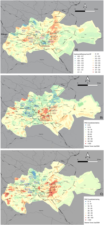
Figure 2. (a) The fractional change ((PM2.5cafter − PM2.5cbefore)/(PM2.5c,before + PM2.5c,after) in predicted PM2.5c after the curfew was imposed, from March 25, 2020 - May 5, 2020, compared to predicted levels before. Estimated PM2.5c values for each 100 m grid-cell in Nairobi (b) before and (c) after the curfew in units of μg m−3 using RF models. The poorer neighborhoods in Nairobi are circled in red and the wealthier neighborhoods are circled in blue. The neighborhoods of Lumumba and Pangani are circled in figure 2(a) in pink as the area of these neighborhoods present in a grid cell are variables with high feature importance in the main RF model.
Download figure:
Standard image High-resolution imageThe predicted estimates of PM2.5c before and during the COVID-19 curfew, as well as the fractional difference between these two periods derived from the two RF models, are displayed in figure 2. The neighborhoods of Nairobi are labeled in figure 2. The mean PM2.5c concentration before the COVID-19 curfew was 23.5 μg m−3 (Median: 22.4 μg m−3). Mean concentration during the COVID-19 curfew was similar: 24.6 μg m−3 (Median: 20.5 μg m−3). A Wilcoxon-rank-sum test revealed no statistically significant differences between the median PM2.5c concentrations in Nairobi overall, before and during the COVID-19 crisis for the time period of this study.
Results from the RF model before and during the COVID-19 curfew using grid-cells with stable PM2.5c concentrations only (Model 2) are displayed in figure S8 in S6.2 in the SI. Results from the universal kriging model (Model 3) are displayed in figure S9 in the SI and described in S6.3 in the SI. Although broadly similar patterns of PM2.5c are observed in the densely sampled city center before and during the COVID-19 curfew in all three models, the patterns of PM2.5c in the outskirts of Nairobi vary markedly across Models 1, 2, and 3. Because of these differences, unlike in the main model, Wilcoxon-rank-sum tests revealed statistically significant differences (Model 2 finds a decrease and Model 3 finds an increase) in the predicted PM2.5c concentrations before and during the COVID-19 crisis. The inconsistencies across models make it impossible for us to robustly describe overall changes in PM2.5c concentrations before and during the COVID-19 crisis in Nairobi.
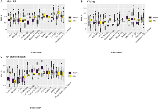
However, certain consistencies in the neighborhood-specific spatial patterns of PM2.5c are observed across all three models. Namely, during both time periods, in all three models, PM2.5c concentrations were higher in places east of the city center in low-income neighborhoods such as Kariobangi, Dandora, Umoja, Mathare and the industrial area (Viwanda) compared to wealthier areas to the west of the central business district, such as Muthaiga, where many embassies are located, and up-scale neighborhoods such as Kilimani, Karura, and Kitisuru (figure 3). These neighborhoods are circled in figure 2 (poor neighborhoods in red and the wealthier neighborhoods in blue). We singled out these neighborhoods as they were densely sampled in both time periods during the mobile monitoring campaign. Wilcoxon-rank-sum tests revealed higher concentrations in Kariobangi, Dandora, Umoja, Mathare, and Viwanda compared to levels in Muthaiga, Kilimani, Karura, and Kitisuru before and after the curfew began across all three models.
Figure 3. Boxplots of predicted PM2.5c concentrations for different sublocations in Nairobi before and after the curfew began for (A): Model 1, (B): Model 2, (C): Model 3. Boxes represent the 25th to 75th percentile, central dark line the median, bars outside the box represent 1.5 x interquartile range, and the circles are the outliers.
Download figure:
Standard image High-resolution image
During the COVID-19 crisis, according to Model 1, PM2.5c concentrations appeared to decrease in the city center. PM2.5c concentrations in the low-income neighborhoods of Umoja, Dandora, and Kariobangi increased. The heaviest increases from both figure 2 appear to be in the rapidly urbanizing neighborhoods of Kahawa and Kasarani in the upper north-east of Nairobi (figure 3). Wilcoxon-rank-sum tests indicate that these increases were significant. Similar patterns and results were obtained from predictions made with Model 3 (figure 3). However, Wilcoxon tests applied to results from Model 2 revealed that the low-income neighborhoods of Umoja, Dandora, and Kariobangi as well as the rapidly growing locations of Kahawa and Kasarani saw significant decreases after the COVID-19 crisis began (figure 3). In all three Models, the industrial area saw significant decreases in PM2.5c concentrations during the COVID-19 crisis (figure 3).
4. Discussion and conclusion
Differences in the spatial variation of PM2.5c before and during the curfew were obtained from all three models (figures 2, S8, and S9). Across predictions from each of the three models considered, the highest concentrations of PM2.5c were seen in certain poor neighborhoods in the locations east of the city center of Nairobi: Mathare, Kariobangi, Umoja, and Dandora in both time periods.
After the curfew was imposed, all three models showed decreases in PM2.5c levels in the industrial area: Viwanda. However, the models provided inconsistent information on overall changes in PM2.5c concentrations, particularly in the outskirts of Nairobi, indicating the need for additional monitoring in these locations to obtain a robust understanding of the spatial variation of PM2.5c levels in Nairobi. No conclusions on the overall changes in PM2.5c in Nairobi can thus be drawn. The models also yielded inconsistent information on the changes in PM2.5c after the curfew was imposed in some of the poorer neighborhoods of Nairobi (Models 1 and 2 yielded a significant increase in PM2.5c concentrations in these neighborhoods while Model 3 indicated a significant decrease).
The bodabodas made few trips to the poorer parts of Nairobi and therefore, these areas were undersampled and the 'generalizable' median PM2.5c concentrations in these locations derived from the mobile monitoring campaign had large errors (figure S7). Measurements in these areas were not used to generate Model 3. It is likely that predictions from Model 3 are not generalizable to these locations due to the particularities of sources and patterns present in these neighborhoods.
Assuming that the measurements in these locations, although noisy, captured overall spatial variations and that Models 1 and 2 are correct, a possible explanation for the increase observed in PM2.5c levels observed in the densely populated, lower-middle-class neighborhoods of Kasarani and Kahawa is that many residents had to switch from LPG to biomass fuel due to loss of income due to the crisis to satisfy their energy needs (Shupler et al 2021). This requires further exploration. The increase observed in PM2.5c concentrations in the poor neighborhoods of Mathare, Kariobangi, Dandora, and Umoja indicates that COVID-19 policies may have exacerbated existing spatial inequalities. This finding suggests the need to understand spatial inequalities better and to use this knowledge to develop improved interventions to support the most vulnerable residents.
'Longitude' had the greatest feature importance in the RF model (Model 1) before the curfew and is second-highest during the curfew. This is also the case for the RF model run on only stable PM2.5c concentrations (Model 2). East of the city center is low-lying, Marshy, and prone to flooding. The 1927 colonial masterplan of Nairobi explicitly states that topography and wind patterns were key considerations in siting the White Highlands to the northwest of the city. Industrial sites, factories, and the African settlements were located in the east. It is likely that the combination of topography, meteorology, and planning reinforced each other to produce the current spatial distribution of PM2.5c in Nairobi. When we compare the prediction results from the RF model and the kriging approach, we find large discrepancies in PM2.5c in the under-sampled neighborhoods of Ruai and Karen, for example. This indicates that sufficient measurements are lacking for these neighborhoods.
Although this experiment yielded several useful insights about the neighborhood-specific spatial variation in PM2.5c concentration in Nairobi before and during the COVID-19 crisis, it has several limitations. We highlight these limitations here and discuss how they might be overcome in future experiments.
One, the mobile measurements used to generate predicted surfaces for Nairobi were made on roads, mostly during the time when movement was allowed in the city. It is possible that during the curfew hours, PM2.5c levels were very different. Thus, the mobile monitoring measurements may not have been temporally representative of values in the locations of monitoring. In future experiments, we hope to use vehicular fleets that are on the road at all hours of the day.
Two, the experiment started on March 16, 2020. The first COVID-19 case in Nairobi was identified on March 13, 2020. In the interim, as news of the virus had spread from other countries, many businesses started operating remotely, and people started leaving the city for their family homes in rural areas. Thus, it is possible that even before the COVID-19 curfew had started, activity was reduced in anticipation of a lockdown. Therefore, the 'before curfew' time period of this study might not truly be representative of conditions during business as normal.
Three, as highlighted in the Results and Discussion, the bodabodas traveled to certain parts of the city more than others (figure S6). This means that certain parts of the city were sampled more than others. The predicted surfaces of PM2.5c we generated were sensitive to the exclusion of data in undersampled neighborhoods. In future experiments, we need to improve the sampling of Nairobi to obtain robust results about the spatial patterns of PM2.5c levels.
Four- many of the covariates used in the RF model were based on data collected in previous years. Several covariates had a relatively coarse resolution. For example, the data on the poverty index at a 1 km × 1 km resolution was for the year 2008, and the land-use map was produced in 2010. There is thus an urgent need to develop open data for the city of Nairobi to further understand intra-city variations of air pollution and other phenomena.
Five, an important limitation of this experiment is that we used low-cost sensors that produced noisy measurements, so the PM2.5 concentrations produced are indicative only. Mass sensitivity of the SPS 30 sensors ranges somewhat across the span of detectable particle sizes but is greatest between 0.3 and 1.3 μm, which is a key range for motor vehicle exhaust near roadways. The error in the reported PM2.5 concentrations will vary somewhat depending on the aerosol size distribution at each moment in time. However, previous studies (as mentioned in section S2.2 in the SI), have shown high reliability between sensors. Our experiment thus allows us to compare the signal from our devices over space. In future experiments, it is important to calibrate such sensors carefully before deploying them. This was not possible for the current experiment, as the data from Nairobi's reference monitor operated by the Kenyan Meteorological Department (KMD) is not publicly available (deSouza 2020). There is thus a need for the government to establish a reference air quality monitoring system that provides high-quality data to residents, which can also be used by researchers.
Despite these limitations, this paper represents the first effort to map out the spatial differences in PM2.5 in Nairobi and to expand upon the environmental justice implications of PM2.5 levels in Nairobi, as well as to discuss the disproportionate impact COVID-19 had on air quality levels across the city. It discusses ways in which future experiments could build on the research design presented to obtain robust insights into neighborhood-specific PM2.5 concentrations.
Acknowledgments
Christoph O Franck, Charles N Christensen, Lorena Gordillo Dagallier, Raphael Jacquat, Sebastian Horstmann and Peter Pihlmann Pedersen would like to acknowledge funding from the University of Cambridge in the framework of the Global Challenges Research Fund (project code: NQAG/244). Open-seneca would like to thank Raphaël Jacquat, Wilkister Mbula, Sue Wairimu, Steve Osumba Ogolla, Christine Otieno, Ishmael Fridah Mwangi, Derrick Mugasia and Ernest Kimani for their support and facilitation of the local project implementation and data collection in Nairobi. We would also like to thank Shin Bin Tan for several useful discussions.
Data availability statement
The data that support the findings of this study are available upon reasonable request from the authors.
Footnotes
- 10
- 11
- 12
Mini-vans which serve as the dominant form of public transport in Nairobi.