
A Macroeconomic SIR Model for COVID-19


Department of Mathematics, University of Michigan, Ann Arbor, MI 48109, USA
*
Author to whom correspondence should be addressed.
†
These authors contributed equally to this work.
Mathematics 2021, 9(16), 1901; https://doi.org/10.3390/math9161901
Submission received: 17 July 2021
/
Revised: 2 August 2021
/
Accepted: 5 August 2021
/
Published: 10 August 2021
(This article belongs to the Special Issue The Mathematics of Pandemics: Applications for Insurance)
Abstract
:The COVID-19 pandemic and subsequent lockdowns highlight the close and delicate relationship between a country’s public health and economic health. Models that combine macroeconomic factors with traditional epidemic dynamics to calculate the impacts of a disease outbreak are therefore extremely useful for policymakers seeking to evaluate the best course of action in such a crisis. We developed a macroeconomic SIR model that considers herd immunity, behavior-dependent transmission rates, remote workers, and the indirect externalities of lockdowns. It is formulated as an exit time control problem where a social planner is able to prescribe separate levels of the lockdown low-risk and high-risk portions of the adult population. The model predicts that by considering the possibility of reaching herd immunity, high-risk individuals are able to leave lockdown sooner than in models where herd immunity is not considered. Additionally, a behavior-dependent transmission rate (which represents increased personal caution in response to increased infection levels) can lower both output loss and total mortality. Overall, the model-determined optimal lockdown strategy, combined with individual actions to slow virus transmission, is able to reduce total mortality to one-third of the model-predicted no-lockdown level of mortality.
1. Introduction
The COVID-19 global pandemic has led to massive lockdowns to slow the spread of the virus. Policymakers faced, and continue to face, a dilemma: extended periods of lockdown have put a strain on the economy, but returning to “normal” too quickly could result in an equally troubling wave of new infections, even with the currently growing vaccine distribution. The task is therefore to find the optimal balance between public health and economic growth. Models such as those proposed by [1,2] have used a macroeconomic approach and variations on the susceptible-infectious-recovered (SIR) epidemic model proposed by [3] to solve an optimization problem determining the lockdown policy that minimizes both the loss of life and the effects on output. We expand on these previous models by presenting our original work, which considers more factors affecting epidemic progression. These novel improvements are listed below and discussed in detail in Section 2:
- We formulated an exit time control problem where lockdown measures are lifted when the population reaches herd immunity;
- We incorporated a transmission rate that captures how individuals react to current infection levels. This “behavior-dependent” transmission rate seeks to model individual behaviors that occur independently of lockdown. For example, individuals might wear masks, practice social distancing, and take other precautions to reduce their risk as infection numbers go up, even in the absence of official lockdown measures;
- We considered the costs of indirect deaths attributed to the adverse mental and physical effects of lockdown and of continued unemployment after the lockdown has ended and the positive impact of workers who are able to work remotely during lockdown;
- We added a penalty for overwhelming intensive care unit (ICU) capacity and a term that captures the future impacts of missed health screenings during the pandemic.
By formulating our problem in such a way, we captured a wider and more accurate picture of the overall situation and found that the inclusion of these elements markedly altered the calculated optimal lockdown strategies.
Literature Review
Epidemic modeling has been a subject of study since the 1700s, and researchers continue to explore new models and approaches, for example those detailed in [4]. The classic susceptible-infected-recovered ODE model [3] is the basis of our (and many other) models, but other approaches have also been taken. Some alternatives include agent-based modeling [5,6], which takes an individual-level approach instead of a population-level one, and metapopulation modeling, which looks at various fragmented populations and their interactions, as in [7]. Motivated by the COVID-19 pandemic, there have been many new additions to the literature in mathematical epidemiology, taking many different approaches. For example, several researchers have taken an individual-level approach, which seeks a mean-field equilibrium. Some notable works include [8,9,10], which compared the mean-field equilibrium to a socially optimal strategy where agents can choose their contact rate and are influenced by various incentives. In addition, data-based approaches such as those in [11,12] have provided interesting insights into targeted lockdowns and the efficacy of stay-at-home orders. In this paper, we chose to manipulate a standard SIR model in order to more easily investigate the effects of added macroeconomic elements, which attempts to capture unique aspects of a modern global pandemic such as COVID-19. This approach is more in line with papers such as [1,2].
The planning problem developed in [1] was the basis of the one used in our model. The paper referenced the SIR method of epidemic modeling, which has also been used in subsequent papers, to represent population dynamics. Many of its parameters, such as the level of obedience to lockdowns, were also used in our model. The death rate was calculated as a function of the number of infected individuals in order to model the effects of hospital overcrowding and encourage “flattening the curve”. The objective function quantifies the economic and social impacts of both the pandemic and the resulting lockdown measures and develops an optimization problem for a planner to solve. The cost of lockdown is represented by the income that is lost by those who are in quarantine and so are unable to work, while the cost of death was calculated as the value of statistical life. Their model examined the role of the population’s level of obedience, as well as the effect of being able to test those who are recovered and excluded them from lockdown. They also investigated the results of different values of statistical life. The authors concluded that being able to test and return recovered individuals to the workforce has a large positive effect on outcomes and that these outcomes are sensitive to the fatality rate and its elasticity with respect to the infection level.
A subsequent paper [2] took this model and extended it by considering the possibility of different optimal lockdown measures for different groups. In their case (and in ours), the groups were differentiated by age, since the severity of COVID-19 infection varies widely based on age. The paper also explicitly considered the number of infected individuals admitted to the ICU at each point in time, which was then used to calculate the death rate. The authors used Pareto curves created by varying the nonpecuniary value of life to show that targeted lockdown measures unilaterally perform better than uniform lockdowns, regardless of whether one seeks to prioritize reducing output loss or reducing mortality. In fact, while they considered three age groups (20–49, 50–64, and 65+), their results showed that it is sufficient to consider a “semitargeted” policy that prescribes one lockdown policy to those aged 20–64 and another policy for those over 65 y. Due to this result, we also split the working population into two groups, one aged 20–64 and one aged 65 and over.
The inclusion of a controllable behavioral parameter that captures the incentives and effects of social distancing has appeared in various game theoretic epidemic models [13,14] and was also recently discussed in [15]. We therefore refer to our model as a behavioral SIR (BSIR) model, because individual behaviors affect infection transmission rates. In both [13,14], the base transmission rate was multiplied by a controlled scale factor between zero and one, which represents the current best-response level of social distancing. In contrast, in our model, the effects of social distancing behaviors were not directly controlled. Rather, the scale factor on the transmission rate fluctuated between zero and one based on the current proportion of infected individuals. This reflects the tendency of individuals to be more careful as infection levels rise in their community.
These works developed a solid framework for our model, but we undertook the task of increasing the accuracy and realism through herd immunity as an exit time, behavior-dependent transmission rates, deaths indirectly due to lockdown, the additional costs of lockdown, and the portion of the population that is able to work remotely. These additions affect the model in various ways, but overall, our augmented model concluded that the high-risk group does not need to maintain a strict and full lockdown for the entire duration of the pandemic when factors such as personal precautionary behaviors and the possibility of herd immunity are included.
The main body of the paper presents our model and its numerical results. In Section 2.1, we lay out the SIR dynamics used to model the transmission of the virus and discuss certain model additions, especially the addition of deaths indirectly caused by lockdown and a behavior-dependent transmission rate. In Section 2.2, we introduce the exit time control problem that ends when the population reaches herd immunity and discuss the terms in the objective function. In Section 3, we discuss our numerical model, which discretizes the problem and is solved through value iterations. We calibrated it with the results of [1,2] and compared these results to our augmented model using death rates on the same scale. Then, we updated the death rates to match more recent data from [16] and adjusted the nonpecuniary value of life. We present and discuss our results and performed some parameter robustness analysis. These experiments serve to illustrate the general mechanisms of the model and to present planners with an idea of our model’s potential. If a planner wishes to experiment with our model, the parameter values can be changed in our code, found at (https://github.com/april-nellis/COVID19-BSIR, accessed on 7 August 2021), to accurately reflect a specific planner’s current situation.
2. Methods
2.1. Population Dynamics
As in [2], we considered policies that assign different lockdown strategies to population groups with different responses to infection and lockdown. Influenced by their results, we divided adults into one group aged 20–64, called “low-risk” and indexed by , and one group aged 65 and over, called “high-risk” and indexed by . We denote the set of population groups as . We only considered adults older than 20, so the low-risk group makes up 82% of the population of interest, while the high-risk group makes up 18% [17]. The second group can also include individuals of any age who are more likely to contract severe cases of COVID-19 and experience complications due to immunodeficiency, respiratory weakness, or other preexisting conditions. These individuals were considered separately from the general working population. We denote the population of group j as a proportion, , of the total population and lay out the following relationship:
Individuals move from susceptible () to infected () to recovered (), with additional flows from all three to death (). The dynamics are given by:
The number of new infections depends on the size of the susceptible and infected populations, as well as the lockdown levels, , and transmission rates between groups, . The lockdown levels were introduced to reduce the number of susceptible individuals who are at risk of being exposed to infection and to reduce the number of infected individuals who are able to infect others. The transmission rate, , is more complex than in the standard SIR model, as the transmission rate varies depending on the interacting populations and also changes in time. It is described in more detail in Section 2.1.2. As others have suggested [1,2] and as history has shown, a portion of the population will disregard lockdown orders. The level of obedience is represented by . As in [2], we set , though this parameter is difficult to quantify exactly. Patients move out of the infected category with rate in accordance with the expected recovery time of 18 d [16]. Deaths due to COVID-19 occur at rate , and other deaths occur at rate . For convenience, the parameters that appear in (1) and in the objective function (2), along with their levels, are listed in Table A1 of the Appendix A.
2.1.1. Deaths
One unique element of COVID-19 is its significantly different death rates for different groups [16]. Therefore, the base death rate for each group was set individually. In addition, as the number of infected individuals increases and hospitals become more crowded, death rates increase as a function of the total number of infected patients as in [1]. We represent this increase in the death rate as and followed [2] in assuming that an infection level of 30% increases the death rate by a factor of five. Therefore, the death rate due to viral infection is:
The number of new deaths due to COVID-19 at a given time must be less than or equal to the total number of individuals removed from the infected category at that time, so we require . Since , this can be achieved by ensuring .
Additionally, as lockdowns stretch on, concerns have been raised regarding “deaths of despair” due to the impacts of lockdowns on mental health [18,19]. Hospitals have also shut down many departments to accommodate the increased need for ICU units for COVID-19 patients. Many nonelective surgeries and routine health checks have also been canceled or rescheduled [20]. This neglect of health maintenance is also very likely to have repercussions on public health. To encompass all this, we added the term , which is written as:
This represents the number of deaths indirectly caused by the lockdown, and scales with . We argue that, in the absence of any way to verify immunity, indirect deaths occur in both the susceptible and recovered populations. Therefore, the total number of deaths is given by:
2.1.2. Behavior-Dependent Disease Transmission
The basic transmission rate of COVID-19 is approximately 0.2 [1,2]. This means that about 20% of those who come in contact with an infected individual will become infected themselves. However, we incorporated a transmission rate that decreases as infections increase due to increased caution between people. In addition, we considered an intergroup interaction factor, , as in [2]. This reflects a lower rate of interactions between groups. For example, working people aged 20–64 will interact more with their peers than with those in the high-risk group. Combining these two ideas, we represent the transmission rate as:
For demonstration purposes, the scale factor in our benchmark model was chosen such that the rate of transmission can be decreased by 25% when 30% of the population is infected with the virus. This could be adjusted after more is known about the viral transmission of particular strains of COVID-19.
2.2. Objective Function
The questions of how long and how severely to lock down the population during a pandemic can be thought of as a planning problem. Given the above dynamics, we modeled the optimization problem that must be solved by a social planner using the following objective function, which represents the overall societal costs of a given lockdown policy:
2.2.1. Attainable Lockdown Levels
There are certain jobs that must be performed even during a pandemic, preventing the population from attaining full lockdown. These essential professions include healthcare workers, grocery store employees, delivery workers, and the postal service, among others. Because of this, we set an upper limit on the possible lockdown level, denoted , and the set of possible lockdown policies is written as . We set at 0.7 to account for essential workers in the low-risk group. On the other hand, was set at 1 since we assumed that the high-risk group does not work.
2.2.2. Herd Immunity
Previous models considered either an infinite time horizon with stochastic vaccine arrival or a fixed horizon with deterministic vaccine arrival when formulating their objective function. We contribute a new approach that sets reaching herd immunity as the end of the problem. This can be reached either naturally via infection spread and recovery (which confers immunity) or via the arrival of a vaccine. We assumed that those who have been infected with COVID-19 once will remain immune for the rest of the outbreak. Additionally, we assumed that if a vaccine is approved for distribution, vaccination levels will be high enough to produce herd immunity, as appears to be the case. We define as the time at which natural herd immunity is reached. We assumed a herd immunity threshold of 60% recovered (In [16], Table 1 (Scenario 5: Current Best Estimates), the basic reproduction number of COVID-19 was . Herd immunity was calculated as .), so we set . Herd immunity achieved through vaccination was incorporated into the model via discounting by , where stochastic vaccine arrival follows an exponential distribution with intensity . While the current situation shows that vaccines arrived in less than 1.5 y, we maintained to remain comparable to previous works [1,2].
2.2.3. Output Loss ()
The most noticeable result of lockdown measures is economic slowdown. Many workers who are not deemed essential and cannot work remotely have found themselves jobless as companies lose revenue. As in [2], we took the average wage of a full-time worker, normalized it to 1, and assumed that, on average, those in the high-risk group do not earn any wages. We did not assume the existence of an “immunity passport” given to those who have recovered, and so assumed they are also subject to lockdown measures. This was accomplished by setting in the expressions below. The parameter p can be instead set to 0 to be consistent with the cases of [1,2], where recovered individuals are not subject to lockdown measures. On the other hand, we considered some proportion h of the workforce who are able to work from home. Therefore, we denote the purely salary-based cost of lockdown as:
When presenting our numerical results, we refer to the output loss due to lockdown. This is not the value of the objective function presented in (2), but rather the losses in output caused by requiring people to stay home and not work. The output loss is represented by:
and is compared to annual “normal” output. This output is calculated as the amount of output produced until the expected vaccine arrival time, , if there were no COVID-19 pandemic and no lockdown, annualized using the expected vaccine arrival time. This is given by:
2.2.4. Cost of Death ()
The main societal concern during a pandemic is the loss of life due to infection, represented in our model by . We calculated the cost of a COVID-19 death in group j in the same manner as in [2]. Here, is the nonpecuniary cost of life, which we considered as a measure of the public impact of deaths due to COVID-19. This can be thought of as a measure of the planner’s priorities. Lower values of lead to prioritizing output loss minimization, while higher values are chosen to encourage longer lockdowns and decrease mortality at the expense of output. To ensure that this cost is on the same order of magnitude as wages, we scaled by the interest rate when choosing , similar to [1]. Note that is consistent with [2], where and . is the number of years left in an average individual’s career. We set and . Therefore, the cost per death due to COVID-19 is given by:
Deaths indirectly caused by lockdown, represented by , are not explicitly categorized and counted, and so can be considered “invisible deaths”. For this reason, we did not include in the cost of these deaths and only counted lost productivity. We also accounted for similar future deaths due to the lack of preventative healthcare using a constant F (the number of indirect deaths in the future relative to those that occur during lockdown). These deaths do not appear in the dynamics, as they have not yet occurred, but they were considered when calculating the costs of lockdown. For this reason, F appears in (2), but not in (1), and the total cost of indirect deaths is given by:
2.2.5. Future Loss of Employment ()
Another addition to the model acknowledges the long-lasting economic impacts of a period of economic slowdown. Large corporations such as JCPenney and Hertz filed for bankruptcy during the initial lockdowns [21] under financial strain [22]. Federal stimulus measures may alleviate some of this burden, but they cannot completely compensate for current drops in consumption. Effects may manifest in a variety of ways, but we chose to express them as a “future loss in employment”, in which one day in lockdown results in some days of lost employment (on average) after lockdown ends. We set this to be 0.42 (reflecting the current 14.7% unemployment rate [23] and assuming an average of 3 d of unemployment for 1 d of lockdown). The cost of future unemployment is modeled by:
2.2.6. ICU Overcapacity ()
A major incentive for lockdown measures is “flattening the curve”—slowing the spread of the virus so that hospitals and ICUs will not become overwhelmed by a flood of patients in need of ventilators and other specialized medical equipment. This is already reflected in the death rate, which increases as infections increase, but we added an additional penalty on top of that. We assumed that a fixed proportion of infected patients, , require ICU care. We set this level to be 2.6% for people without underlying conditions and 7.4% for high-risk groups [16]. Then, we incorporated a penalty (representing a daily penalty scaled by the level of overcapacity) for hospitalizations exceeding the estimated average ICU capacity, which is 30 beds per 100,000 people [24]. This is performed via the function:
3. Numerical Results
3.1. Numerical Method
We used value iterations, first introduced by [25], to solve the optimization problem presented by our model. The model was discretized using first-order Taylor approximations, and the value function was calculated over a regular grid. Because the change in population due to deaths is very small, we followed the precedent set in [1] and iterated over a four-dimensional grid to determine the optimal lockdown policy instead of the larger and more computationally expensive (but more accurate) six-dimensional grid . By this, we mean that instead of separately keeping track of the recovered and dead populations, they were considered together as one unit when determining the optimal lockdown policy. Since the vast majority of this “nonsusceptible” group is recovered, this simplification, which removes two state variables, has a small effect on accuracy, but a large effect on computational complexity. When determining the pandemic trajectory for given initial conditions and a given lockdown policy, total deaths can still be calculated via the population dynamics shown in (1). We chose and in our discretization and set days as the unit of time. For all models, we took the initial conditions to be uniform across groups (if applicable) and set them at the level of 98% susceptible, 1% infected, and 1% recovered, unless otherwise specified.
3.2. Calibration
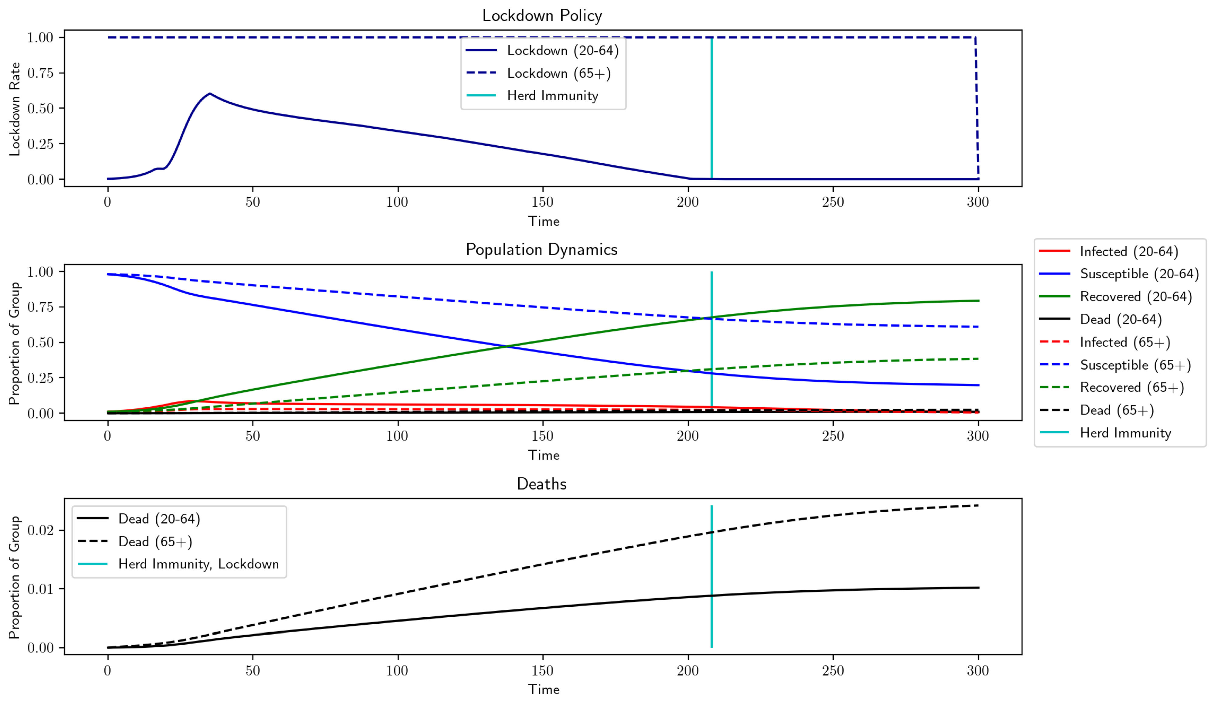
To test the validity of our numerical models, we used the parameter values of [1,2] and compared our model’s recommendations to their results. A full list of the parameter values used in this section is presented in Table A1. In Figure 1, we compare a one-group version of our model with the one presented in [1], whose recommended optimal lockdown reached 70% lockdown after about one month and then slowly reduced in intensity until lockdown was lifted approximately 140 d (4.5 mo) after the outbreak began. Our version of this model maintains the maximum lockdown of 70% for slightly longer and ends slightly later. Interestingly, the ending of lockdown nearly coincides with the population reaching herd immunity, though we did not add any such considerations when running this example. In Figure 2, we set up our model to mimic the semitargeted policy from [2] and to find similar levels of output loss, total deaths, and general lockdown recommendations. Namely, the optimal strategy keeps the high-risk group in lockdown until the arrival of a vaccine, while the low-risk group is able to emerge and return to work after approximately 200 d of lockdown have elapsed. In this figure, note that the population reaches herd immunity well before the arrival of a vaccine, implying that the lockdown on the high-risk group could have been ended earlier.
Now, we investigate the results of our new model using comparable parameter levels. We incorporated herd immunity, deaths indirectly due to lockdown, the ability to work remotely, and behavior-dependent transmission rates. Additionally, we considered the possibility of lost employment after the end of the pandemic, as well as the costs of missed health screenings and a monetary penalty for exceeding ICU capacity. To allow comparisons with previous works, we used death rates of a similar magnitude to those in [1,2], but we changed some parameters to better fit the current situation. Interest rates have dropped significantly, so we used a 0.001% interest rate, instead of the 5% used by [1] or the 1% used by [2]. Note that since the interest rate is extremely low, there was little to no discounting applied to wages. We also lengthened the projected average career length in the low-risk group. Finally, we adjusted the population distribution slightly from 21% high-risk to 18% high-risk, based on data from the 2010 United States Census [17]. The results of our model using the parameters listed in Table A1 are shown in Figure 3. Most noticeably, lockdown rates for both groups fall to zero after the entire population reaches herd immunity, which was explicitly imposed by our model. Additionally, the lockdown for the low-risk group is slightly shorter, but more intense. Unsurprisingly, incorporating deaths of despair increases the total number of deaths due to the pandemic, but this effect is kept small by the shorter lockdowns. Long-term costs of lockdown (an additional penalty for ICU overcrowding, future deaths due to current health negligence, and future unemployment beyond the lockdown) increase output loss while not directly contributing to deaths during lockdown. However, these output losses are offset by the proportion of the population that is able to work remotely from home and the shorter lockdown periods.
3.2.1. Realistic Death Rates
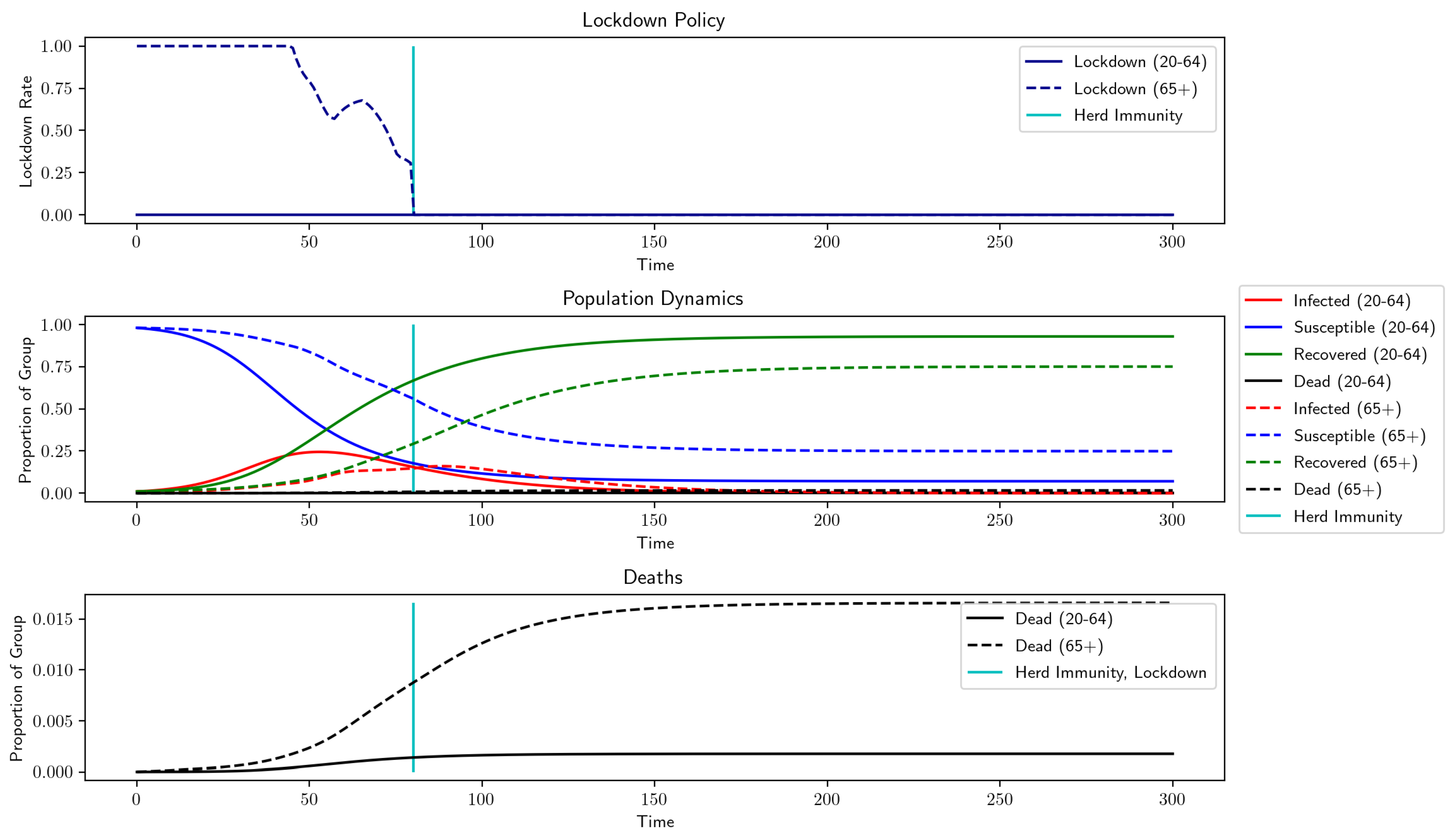
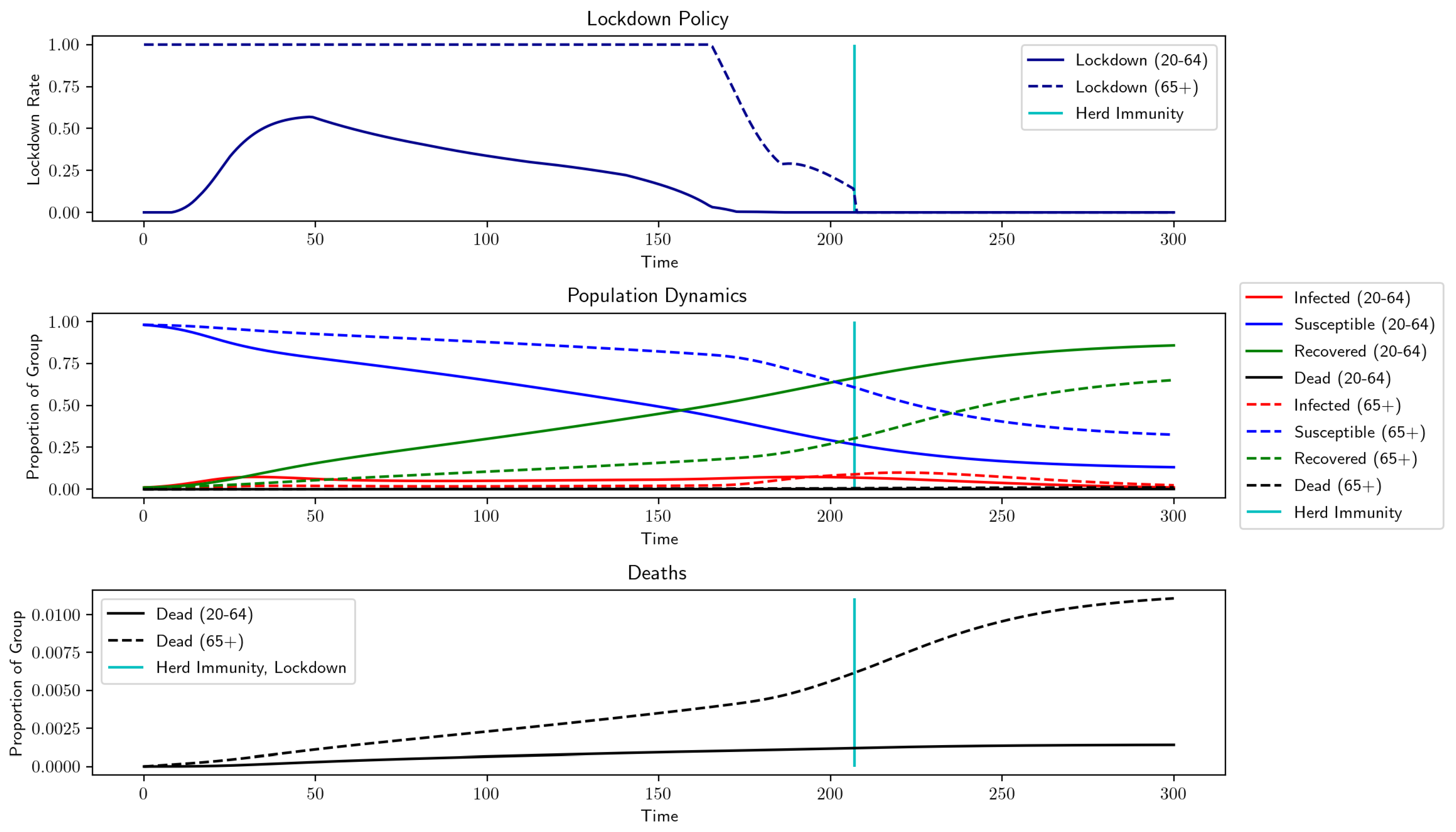
Recent CDC reports [16] indicate that the death rates are much lower than those used in Section 3.2. To increase the realism of our model, we updated the model death rates according to this newer data (We calculated death rates based on the data in [16], Table 1 (Scenario 5: Best Current Estimates). To calculate , we constructed a weighted average of the symptomatic case fatality ratio for 0–49 year-olds and for 50–64 year-olds using the 2010 Census data [17] and multiplied by 0.65, since the CDC estimates that 35% of cases are asymptomatic. For the same reason, we multiplied the symptomatic case fatality ratio for the 65+ group by 0.65 to determine . We set such that a 30% infection level causes a five-fold increase in deaths, as in [2], and used them for all subsequent results. These death rates are listed in Table 1, and the result, shown in Figure 4, predicts a total mortality of 0.4464% and a total output loss of 0.0013%. The negligible output loss is due to the negligible lockdown for the low-risk group. However, lockdowns have already been imposed for both groups (and indeed, we might desire a death rate lower than 0.4464%), so we increased the nonpecuniary value of life, , and observed how the model changes. By increasing from to , Figure 5 shows that both groups experience levels of lockdown similar to that of Figure 3, but with an output loss of 4.8984% and a lower total death toll of only 0.3266%. We designate this the benchmark situation, which uses the death rates from Table 1 and , but keeps all other parameter values are consistent with those in Table A1. We also compared the results of the optimal lockdown to those generated by an uncontrolled scenario with the same parameters, shown in Figure 6 and Table 2. Without lockdown, there is no output loss, but final mortality numbers are approximately twice as high.
3.2.2. Varying Initial Conditions
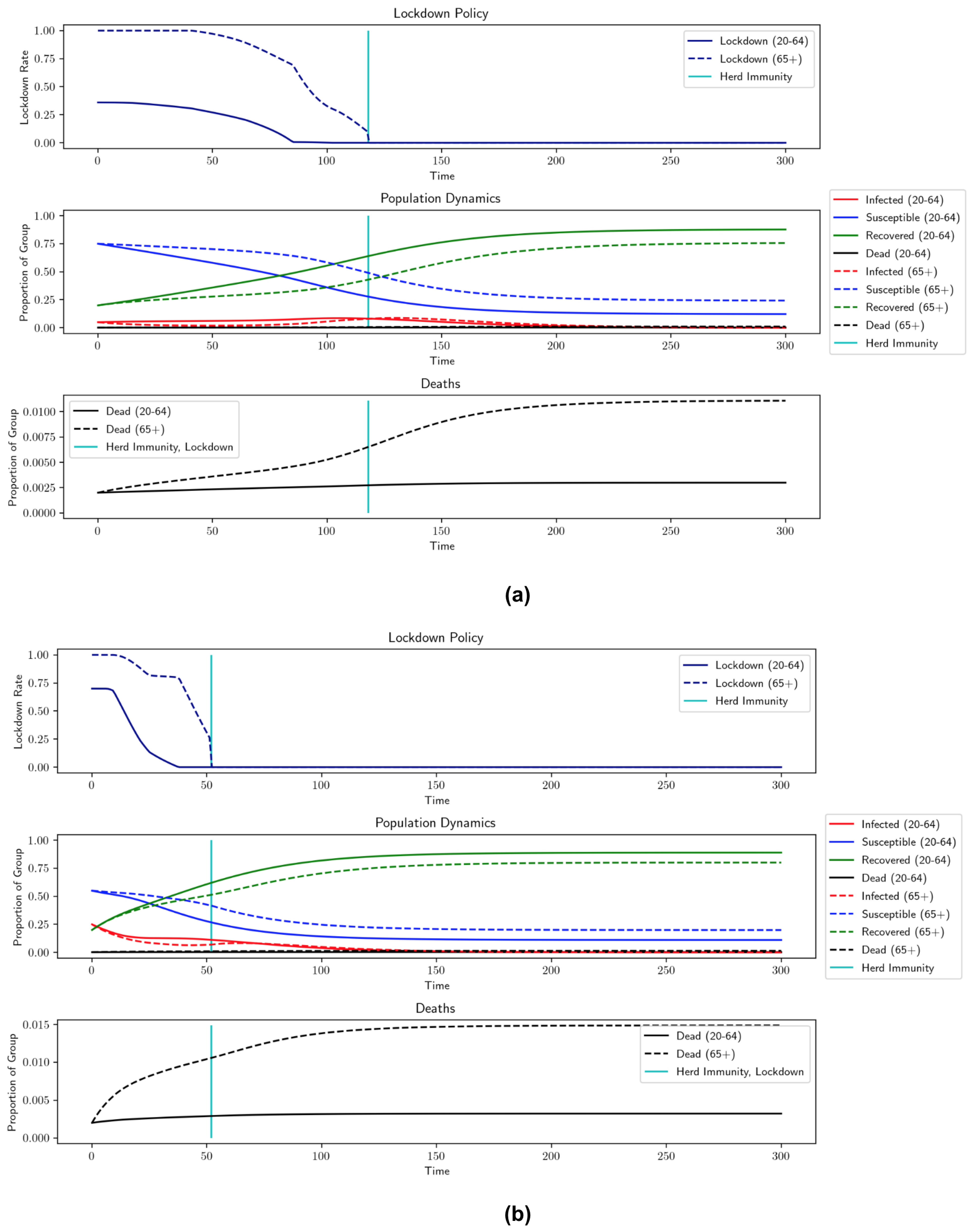
Since we are currently in the middle of the pandemic, we investigated how different initial conditions change the recommended lockdown levels. We modeled a situation where the pandemic is ongoing and lockdown measures have been lifted, but a sudden spike in infections occurs that prompts new lockdown measures. We considered a case where 20% of the population has recovered and 0.2% has died, similar to the estimates of the current situation in New York City [26]. In Figure 7a, a small infection spike affects 5% of the population before lockdown measure are put in place. In this case, we see additional deaths of 0.2452%. In Figure 7b, a large infection spike affects 25% of the population, causing 0.3346% additional deaths. Note that the lockdown is actually shorter for larger infection spikes, since the larger infection level (which occurs before lockdowns are imposed) moves the population closer to herd immunity. The price of this shorter lockdown, though, is higher mortality rates.
3.3. Parameter Robustness and Discussion
It is natural to ask how changes in other parameters affect the optimal controls. In general, changes in parameters create the expected changes in lockdown length and intensity, output loss, and mortality. The more interesting question asks about the level of impact of various parameters. The effects of the nonpecuniary value of life () have already been discussed and are displayed in Figure 4 and Figure 5 and Table 3, but now, we discuss other parameters. In Table 4, we list the lockdown levels, mortality, and output loss for various other configurations of parameter choices.
There are some elements of the model that did not have large impacts on the results. The ICU overcapacity constraint barely affected the results, likely due to a combination of low infection rates and a sufficiently high number of ICU beds (on average) in the United States. This allows ICU admittance rates to remain at or below the threshold. The expected vaccine arrival date also did not have much effect on the optimal lockdown levels, since the population is expected to reach herd immunity well before its introduction. To acknowledge that multiple vaccines have already begun circulating, we also considered expected vaccine arrival times of 1 y () and 8 mo () and found that neither adjustment had much effect. It can also be seen from the table that removing F, the cost representing future deaths due to the current lack of health maintenance lengthens the lockdown only slightly and has little effect on output loss and mortality.
In contrast, loss of future employment, ability to work remotely, indirect death rate in lockdown, intergroup interaction, and behavior-dependent infection transmission have significant effects on lockdown length and severity. Adding output savings from remote work, future employment loss due to lockdown, and indirect deaths of lockdown affects the wider population, and so produces similar changes in the outcomes. The model produces uniformly better outcomes when the level of remote work, h, is increased, though lockdowns do last longer, as seen in Figure 8. Intuitively, this follows from the idea that more people working remotely helps to maintain economic activity without increasing the risk of infection. Changing and in the opposite direction of remote work creates similar effects on the optimal lockdown policy, though outcomes move differently. Increasing the length of projected future unemployment, , leads to a shorter lockdown and less output loss, while deaths increase. This suggests that influences the trade-off between output loss and mortality. When we look at varying values of , we can see what happens when the optimization tries to minimize deaths due to COVID-19 while also trying to avoid deaths due to lockdown. When and the model does not take indirect deaths into account, the lockdown extends for longer and has a larger effect on output, but we see much lower mortality levels. However, when is increased to 50 deaths per 100,000 individuals at full lockdown, the model dramatically shortens the lockdown, which decreases output loss and indirect deaths, but leads to higher deaths due to COVID-19. Accurately determining the true value of this parameter is therefore of high importance when developing a policy based on our model.
We now discuss the effects of behavior-related parameters. Interestingly, these are the only parameters we discuss that also have an effect on the uncontrolled outcomes. If the level of interaction between groups, , is lowered, there is less interaction between the low-risk and high-risk groups, and so, lockdowns are more effective. In Figure 9, when goes from 0.75 to 0.5, the low-risk group is able to begin easing the lockdown earlier since there is less worry about transmission to high-risk individuals. However, the lockdown lasts longer overall, since it is harder to reach herd immunity. This increase in output is offset by a drop in mortality. With the optimal lockdown, mortality decreases to 0.2552% compared to the benchmark of 0.3166% when . With no lockdown, mortality decreases to 0.5268% from 0.6189%. The opposite occurs when is increased to one, meaning that the groups mix freely. Herd immunity arrives sooner due to increased intergroup transmission; however, mortality increases to 0.3599% with lockdown and to 0.6891% without it. This suggests that it is beneficial for high-risk individuals to exercise extra caution in their interactions with members of the low-risk group. The other parameter that reflects individual behavior, , also has a notable impact on optimal lockdown policies. This parameter determines the efficacy of personal actions taken to slow the transmission of COVID-19. In the benchmark case, . If transmission rates are constant (), then the lockdown lasts longer due to the increased likelihood of transmission and mortality increases to 0.3394%. In the uncontrolled case, the mortality increases as well, to 0.7586%. However, if is set very high (say 10, which implies that personal caution can reduce the transmission rate by 95% when infections reach 30%), then a lockdown is barely necessary, as shown in Figure 10. In this case, uncontrolled mortality is a mere 0.2581%. This second scenario is perhaps too optimistic, but it demonstrates the potential power of social distancing. If we examine and , we see that the lockdowns increase as decreases. If we consider the more modest change from to and decrease the interaction level between groups from to , then imposing the optimal lockdown decreases overall mortality from 0.7586% to 0.2552%. This implies that taking measures to reduce transmission during social interactions, in addition to reducing the number of interactions, can play a major role in controlling disease spread.
If the population is less obedient and disregards lockdown measures, for example if decreases from 0.75 to 0.6, we see that the lockdown is shorter because herd immunity is reached sooner. This decreases output loss, but leads to more deaths. If the population is more obedient, however, for example if , the effect of a given level of lockdown is larger with respect to the same level of output loss, so lockdowns are less intense, but last longer. The arrival of herd immunity is slower, leading to higher output loss, but the strategy has the benefit of lower mortality. This is because the same level of output is lost for a given lockdown rate, regardless of , and so, higher obedience levels result in a lockdown being more “worth” the output loss; therefore, the algorithm allows a slightly higher output loss in order to achieve much lower mortality rates. This implies that if a lockdown is enacted, for maximum efficiency, it should be correctly incentivized in order to achieve high obedience.
Finally, in Figure 11, we investigate the effect of more conservative herd immunity thresholds . In all the examples, the low-risk group is able to leave lockdown before the arrival of herd immunity, so moving the threshold does not have much impact on output loss. However, has important implications for the high-risk group. From Figure 11, we see that there is a clear change in the dynamics for thresholds of 75% and above. The length of lockdown for the low-risk group increases by about 20 d, but the high-risk group remains in lockdown until the vaccine arrives—an increase of almost 300 d. This abrupt change in strategy arises because eventually, the population reaches a steady state with very low infections, so basically, it reaches herd immunity. This reflects the relationship between herd immunity and transmission rates and indicates that the herd immunity threshold has been overestimated. If the herd immunity threshold is 100%, this is equivalent to removing the herd immunity exit time. The impact of including can therefore be observed as a decrease in output loss and an increase in mortality, while decreasing lockdown length for the high-risk group by 340 d and for the low-risk group by 45 d.
4. Conclusions
We presented a realistic model of pandemic modeling that incorporates previously unconsidered factors such as natural herd immunity, behavior-dependent transmission rates, and indirect deaths due to lockdown, and thereby extends previous models, resulting in markedly different lockdown recommendations. The most notable difference was shorter lockdowns, due to the hope of reaching herd immunity and the cost of indirect deaths as an additional penalty on lengthy lockdowns. This strategy did result in lower levels of output loss, but it also resulted in higher mortality rates, especially among the high-risk population. Our major results can be summarized as follows:
- When the expected vaccine arrival time is 1.5 y after the start of the outbreak, our model recommends less than 7 mo of lockdown for the high-risk group (instead of locking down for the full 1.5 y until the vaccine). Additionally, lockdowns for the low-risk group are 6 wk shorter than in previous models. This means that there are ways of slowing community spread of COVID-19 to protect high-risk individuals;
- The addition of a behavior-dependent virus transmission rate contributes to these shorter lockdowns and decreases mortality. In an extreme situation where individuals can take measures that decrease transmission by 95% when infections reach 30%, less than a month of lockdown is prescribed for the low-risk group. In the more moderate benchmark case, where individuals are able to reduce their transmission by 25% when infections reach 30% of the population, herd immunity arrives a month earlier than in a situation with a constant disease transmission rate. In both cases, we also observe lower output loss due to shorter lockdown and fewer deaths due to slower transmission;
- Increasing the predicted length of future unemployment and the predicted rate of lockdown-related deaths both decrease lockdown length in similar manners and have negative impacts on outcomes. Adjusting the length of future unemployment and the predicted number of indirect deaths due to lockdown leads to trade-offs between output and mortality. Running the model with different initial conditions shows that higher prelockdown infection levels lead to earlier onset of herd immunity, but higher death tolls, highlighting the risks of infection spikes. Future impacts of current missed health screenings and a penalty for overfull ICUs are revealed to have little impact on the optimal lockdown policy in our formulation;
- Increasing the level of remote work reduces the impact of COVID-19 by decreasing both mortality and output loss, even though a longer lockdown is imposed. This supports the intuitive idea that increased remote work reduces infection risk without sacrificing economic activity.
In addition, when comparing between our proposed model and our implementation of the model described in [1], using the same parameters, output loss was reduced by 1.0909% and lockdowns for the high-risk population ended after 211 d instead of the expected 540, while mortality was increased by 0.5752% (in absolute terms). The social planner would have to consider whether this tradeoff is desirable. However, incorporating a behavior-dependent transmission rate that reflects the effects of using personal protective equipment and social distancing could result in shorter lockdowns and lower mortality rates. As expected, reduced disease transmission results in unequivocally better outcomes and should be a priority for policymakers.
In the future, we could expand this model in a variety of ways. The SIR model is a very simple and elegant method of modeling disease transmission, but has its drawbacks because of this lack of complexity. For example, Reference [27] reported inaccuracies when applying SIR models to a case study on the city of Isfahan. More complicated models, such as those that take into account fading immunity over time (SIRS) or include an incubation period (SEIR), could be used to further increase the accuracy of the model. However, Reference [28] found that an SIR model performed better than the more complex SEIR model when matching model predictions to real-world COVID-19 data. Therefore, the efficacy of SIR models is still a topic of discussion in the scientific community. Other considerations, such as low vaccination rates, could also be considered when modeling the “end” of the pandemic and trying to determine the appropriate lockdown length. Multiple strains of a disease with different transmission rates, or different transmission methods, could also be incorporated to generalize our model. In this vein, we could further increase the realism of the model by inserting some element of stochasticity into the SIR dynamics, either through a stochastic transmission rate or by replacing the current deterministic disease progression by Levy processes. However, we believe that the current formulation strikes a good balance between being specific enough for accuracy and being general enough for flexibility.
Author Contributions
Conceptualization, E.B., A.C. and A.N.; methodology, E.B., A.C. and A.N.; software, A.N.; validation, E.B., A.C. and A.N.; formal analysis, E.B., A.C. and A.N.; investigation, E.B., A.C. and A.N.; resources, E.B., A.C. and A.N.; writing—original draft preparation, E.B., A.C. and A.N.; writing—review and editing, E.B., A.C. and A.N.; visualization, A.N.; supervision, E.B. and A.C. All authors have read and agreed to the published version of the manuscript.
Funding
E. Bayraktar was funded in part by the National Science Foundation under Grant DMS-2106556 and by the Susan M. Smith Chair. The research of A. Cohen is supported by the National Science Foundation (DMS-2006305).
Institutional Review Board Statement
Not applicable.
Informed Consent Statement
Not applicable.
Data Availability Statement
Not applicable.
Acknowledgments
We thank the anonymous AE and the three referees for their suggestions, which helped us improve our paper.
Conflicts of Interest
The authors declare no conflict of interest.
Appendix A

Table A1.
Full list of parameters.
| Parameter | Description | Our Model | ||
|---|---|---|---|---|
| Maximum attainable lockdown | 0.7 | [0.7, 0.7, 1] | [0.7, 1] | |
| Recovery rate | 1/18 | 1/18 | 1/18 | |
| Base mortality | 0.01 | |||
| Rate of mortality increase based on infection levels | 0.05 | if I = 30%, then mortality rates are 5 times the base rates | ||
| Rate of ICU admittance | N/A | (unknown) | [0.026, 0.074] | |
| ICU capacity as the proportion of the overall population (based on beds/100,000 individuals) | N/A | N/A | 0.0003 | |
| Scale factor for the cost of ICU overcapacity | N/A | N/A | 10 | |
| Initial transmission rate | 0.2 | 0.2 | 0.2 | |
| Interaction level between groups | N/A | 1 | 0.75 | |
| Intensity for vaccine/cure arrival | 0.667/365 (1.5 yrs) | 0.667/365 | 0.667/365 | |
| Normalized individual daily productivity | 1 | [1, 1, 0] | [1, 0] | |
| h | Proportion of the workforce that can work remotely | 0 | 0 | 0.4 |
| r | Yearly interest rate | 5% | 1% | 0.001% |
| Nonpecuniary cost of death | 0 | 20 | 0.2/r | |
| Years left in career | ∞ | [15, 7.5, 0] | [20, 0] | |
| Obedience to lockdown | 0.5 | 0.75 | 0.75 | |
| Scaling factor for indirect deaths due to lockdown | 0 | 0 | 0.00001 | |
| Scaling factor for decrease in due to personal social distancing measures (masks, etc.) | 0 | 0 | 1 | |
| Scale factor for decreasing potential career length/increasing chance of bankruptcy as lockdown lengthens | N/A | 0 | 0.01 | |
| F | Future cost of missing health maintenance during lockdown | 0 | 0 | 1 |
| p | Immunity passport p = 1 ⇒ no passport p = 0 ⇒ passport | 0 | 0 | 1 |
References
- Alvarez, F.E.; Argente, D.; Lippi, F. A Simple Planning Problem for COVID-19 Lockdown, Testing, and Tracing. Am. Econ. Rev. Insights 2021, 3. [Google Scholar] [CrossRef]
- Acemoglu, D.; Chernozhukov, V.; Werning, I.; Whinston, M.D. Optimal Targeted Lockdowns in a Multi-Group SIR Model. Am. Econ. Rev. Insights 2021, 3. [Google Scholar] [CrossRef]
- Kermack, W.O.; McKendrick, A.G.; Walker, G.T. A contribution to the mathematical theory of epidemics. Proc. R. Soc. Lond. Ser. A 1927, 115, 700–721. [Google Scholar] [CrossRef] [Green Version]
- Nowzari, C.; Preciado, V.M.; Pappas, G.J. Analysis and Control of Epidemics: A Survey of Spreading Processes on Complex Networks. IEEE Control Syst. Mag. 2016, 36, 26–46. [Google Scholar] [CrossRef] [Green Version]
- Ajelli, M.; Gonçalves, B.; Balcan, D.; Colizza, V.; Hu, H.; Ramasco, J.J.; Merler, S.; Vespignani, A. Comparing large-scale computational approaches to epidemic modeling: Agent-based versus structured metapopulation models. BMC Infect. Dis. 2010, 10, 190. [Google Scholar] [CrossRef] [Green Version]
- Ajelli, M.; Merler, S. An individual-based model of hepatitis A transmission. J. Theor. Biol. 2009, 259, 478–488. [Google Scholar] [CrossRef] [Green Version]
- Colizza, V.; Vespignani, A. Epidemic modeling in metapopulation systems with heterogeneous coupling pattern: Theory and simulations. J. Theor. Biol. 2008, 251, 450–467. [Google Scholar] [CrossRef] [Green Version]
- Aurell, A.; Carmona, R.; Dayanikli, G.; Lauriere, M. Optimal incentives to mitigate epidemics: A Stackelberg mean field game approach. arXiv 2021, arXiv:2011.03105. [Google Scholar]
- Cho, S. Mean-Field Game Analysis of SIR Model with Social Distancing. arXiv 2020, arXiv:2005.06758. [Google Scholar]
- Elie, R.; Hubert, E.; Turinici, G. Contact rate epidemic control of COVID-19: An equilibrium view. Math. Model. Nat. Phenom. 2020, 15, 35. [Google Scholar] [CrossRef]
- Fowler, J.H.; Hill, S.J.; Levin, R.; Obradovich, N. Stay-at-home orders associate with subsequent decreases in COVID-19 cases and fatalities in the United States. PLoS ONE 2021, 16, e0248849. [Google Scholar] [CrossRef] [PubMed]
- Fokas, A.; Cuevas-Maraver, J.; Kevrekidis, P. Easing COVID-19 lockdown measures while protecting the older restricts the deaths to the level of the full lockdown. Sci. Rep. 2021, 11, 5839. [Google Scholar] [CrossRef] [PubMed]
- Reluga, T.C. Game Theory of Social Distancing in Response to an Epidemic. PLoS Comput. Biol. 2010, 6, e1000793. [Google Scholar] [CrossRef] [PubMed]
- Choi, W.; Shim, E. Optimal strategies for vaccination and social distancing in a game-theoretic epidemiologic model. J. Theor. Biol. 2020, 505, 110422. [Google Scholar] [CrossRef] [PubMed]
- Cochrane, J. An SIR Model with Behavior. 2020. Available online: https://johnhcochrane.blogspot.com/2020/05/an-sir-model-with-behavior.html (accessed on 4 June 2020).
- CDC. COVID-19 Pandemic Planning Scenarios. 2020. Available online: https://www.cdc.gov/coronavirus/2019-ncov/hcp/planning-scenarios.html#table-1 (accessed on 7 June 2020).
- Howden, L.; Meyer, J. Age and Sex Composition: 2010. 2010. Available online: https://www.census.gov/prod/cen2010/briefs/c2010br-03.pdf (accessed on 4 June 2020).
- Zhang, S.X.; Wang, Y.; Rauch, A.; Wei, F. Unprecedented disruption of lives and work: Health, distress and life satisfaction of working adults in China one month into the COVID-19 outbreak. Psychiatry Res. 2020, 288, 112958. [Google Scholar] [CrossRef] [PubMed]
- Elmer, T.; Mepham, K.; Stadtfeld, C. Students under Lockdown: Assessing Change in Students Social Networks and Mental Health during the COVID-19 Crisis. PLoS ONE 2020. Available online: https://journals.plos.org/plosone/article?id=10.1371/journal.pone.0236337 (accessed on 4 June 2020). [CrossRef] [PubMed]
- Soreide, K.; Hallet, J.; Matthews, J.B.; Schnitzbauer, A.A.; Line, P.D.; Lai, P.; Otero, J.; Callegaro, D.; Warner, S.G.; Baxter, N.N.; et al. Immediate and Long-Term Impact of the COVID-19 Pandemic on Delivery of Surgical Services. Br. J. Surg. 2020, 107, 1250–1261. [Google Scholar] [CrossRef]
- Monica, P.R.L. Beware of Bankrupt Stocks Like JCPenney and Hertz. 2020. Available online: https://www.cnn.com/2020/05/28/investing/bankruptcies-stocks-jcpenney-hertz/index.html (accessed on 7 June 2020).
- Bartik, A.W.; Bertrand, M.; Cullen, Z.; Glaeser, E.L.; Luca, M.; Stanton, C. The impact of COVID-19 on small business outcomes and expectations. Proc. Natl. Acad. Sci. USA 2020, 117, 17656–17666. [Google Scholar] [CrossRef]
- BLS. The Employment Situation—April 2020. 2020. Available online: https://www.bls.gov/news.release/pdf/empsit.pdf (accessed on 4 June 2020).
- Prin, M.; Wunsch, H. International comparisons of intensive care: Informing outcomes and improving standards. Curr. Opin. Crit. Care 2012, 18, 700–706. [Google Scholar] [CrossRef] [Green Version]
- Bellman, R. A Markovian decision process. J. Math. Mech. 1957, 6, 679–684. [Google Scholar] [CrossRef]
- State, N.Y. Amid Ongoing COVID-19 Pandemic, Governor Cuomo Announces Results of Completed Antibody Testing Study of 15,000 People Showing 12.3 Percent of Population Has COVID-19 Antibodies. 2020. Available online: https://www.governor.ny.gov/news/amid-ongoing-covid-19-pandemic-governor-cuomo-announces-results-completed-antibody-testing (accessed on 19 June 2020).
- Moein, S.; Nickaeen, N.; Roointan, A.; Borhani, N.; Heidary, Z.; Javanmard, S.; Ghaisari, J.; Gheisari, Y. Inefficiency of SIR models in forecasting COVID-19 epidemic: A case study of Isfahan. Sci. Rep. 2021, 11, 4725. [Google Scholar] [CrossRef] [PubMed]
- Roda, W.C.; Varughese, M.B.; Han, D.; Li, M.Y. Why is it difficult to accurately predict the COVID-19 epidemic? Infect. Dis. Model. 2020, 5, 271–281. [Google Scholar] [CrossRef] [PubMed]
Figure 1.
Our implementation of the model of [1] (no groups or herd immunity); parameters from Table A1. Output loss: 13.4232%, total deaths: 1.1754%.

Figure 2.
Our implementation of the model of [2] (two groups and no herd immunity); parameters from Table A1. Output loss: 8.9676%, total deaths: 1.3121%.

Figure 3.
Proposed model (two groups, herd immunity); parameters from Table A1. Herd immunity: 211 d, output loss: 7.8767%, total deaths: 1.8873%.
Figure 3.
Proposed model (two groups, herd immunity); parameters from Table A1. Herd immunity: 211 d, output loss: 7.8767%, total deaths: 1.8873%.

Figure 4.
Proposed model with lower death rates from Table 1 (, all others from Table A1). Herd immunity: 80 d, output loss: 0%, total deaths: 0.4464%.

Figure 5.
Benchmark—herd immunity: 207 d, output loss: 7.3439%, total deaths: 0.3266%. Benchmark parameters: , , , , , , , , , , . Death rates from Table 1. Herd immunity = 60%.
Figure 5.
Benchmark—herd immunity: 207 d, output loss: 7.3439%, total deaths: 0.3266%. Benchmark parameters: , , , , , , , , , , . Death rates from Table 1. Herd immunity = 60%.

Figure 6.
Comparison of optimal lockdown policy to no lockdown, using benchmark parameters. Optimal lockdown deaths: 0.3266% vs. uncontrolled deaths: 0.6189%.
Figure 6.
Comparison of optimal lockdown policy to no lockdown, using benchmark parameters. Optimal lockdown deaths: 0.3266% vs. uncontrolled deaths: 0.6189%.

Figure 7.
Results for varied initial conditions using benchmark parameters. (a) , lockdown: 118 d, output loss: 3.4677%, additional deaths: 0.2452%; (b) , lockdown: 52 d, output loss: 2.1755%, additional deaths: 0.3346%.
Figure 7.
Results for varied initial conditions using benchmark parameters. (a) , lockdown: 118 d, output loss: 3.4677%, additional deaths: 0.2452%; (b) , lockdown: 52 d, output loss: 2.1755%, additional deaths: 0.3346%.

Figure 8.
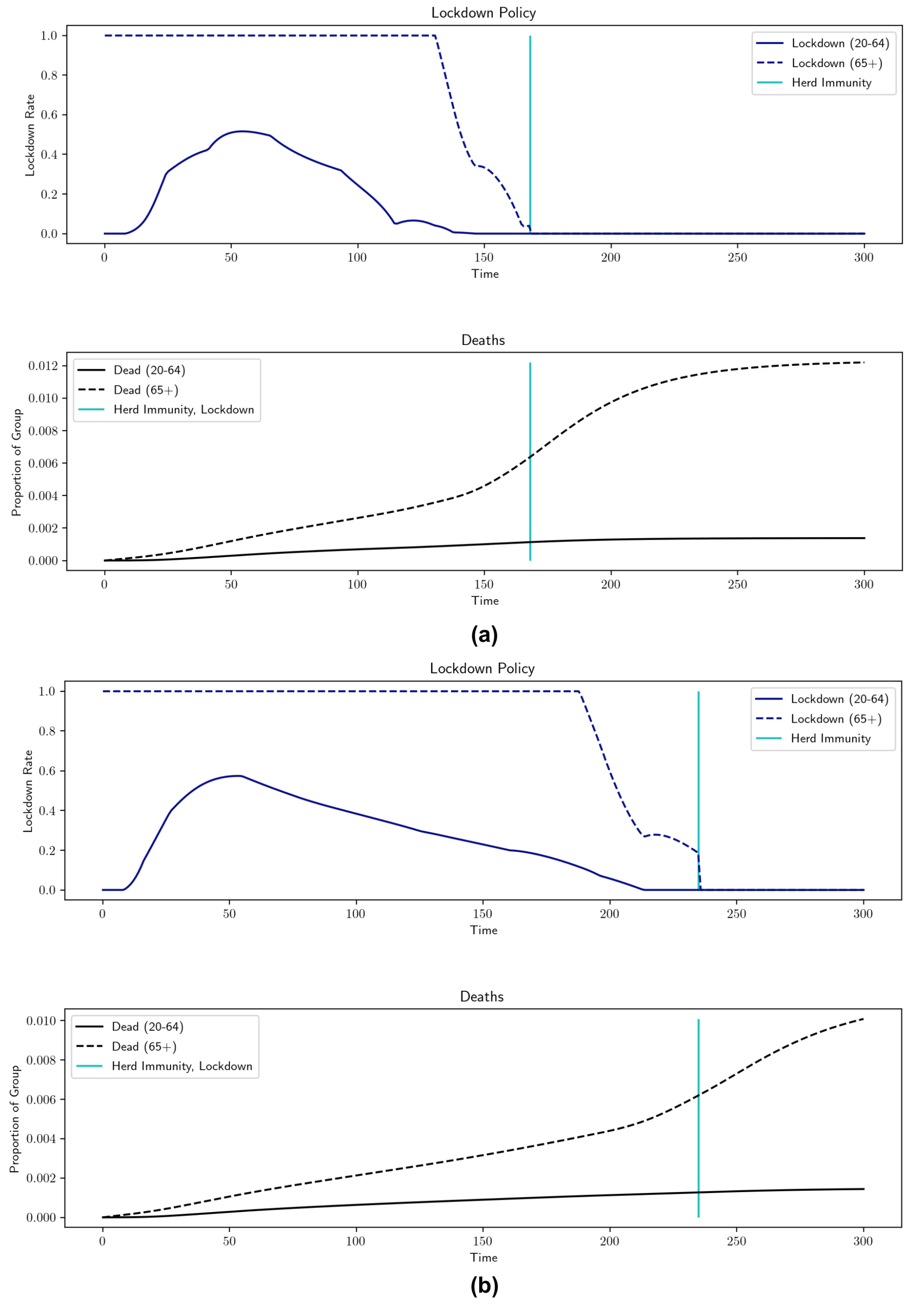
Robustness results for h (percentage of workforce that can work remotely). , , , , , , , , . (a) , lockdown: 168 d, output loss = 8.8592%, total deaths = 0.338%; (b) , lockdown: 235 d, output loss = 5.842%, total deaths = 0.3251%.
Figure 8.
Robustness results for h (percentage of workforce that can work remotely). , , , , , , , , . (a) , lockdown: 168 d, output loss = 8.8592%, total deaths = 0.338%; (b) , lockdown: 235 d, output loss = 5.842%, total deaths = 0.3251%.

Figure 9.
Robustness results for (inter-group interaction level). , , , , , , , , , (a) , lockdown: 233 d, output loss = 8.118%, total deaths = 0.2753%; (b) , lockdown: 194 d, output loss = 7.0292%, total deaths = 0.3657%.
Figure 9.
Robustness results for (inter-group interaction level). , , , , , , , , , (a) , lockdown: 233 d, output loss = 8.118%, total deaths = 0.2753%; (b) , lockdown: 194 d, output loss = 7.0292%, total deaths = 0.3657%.

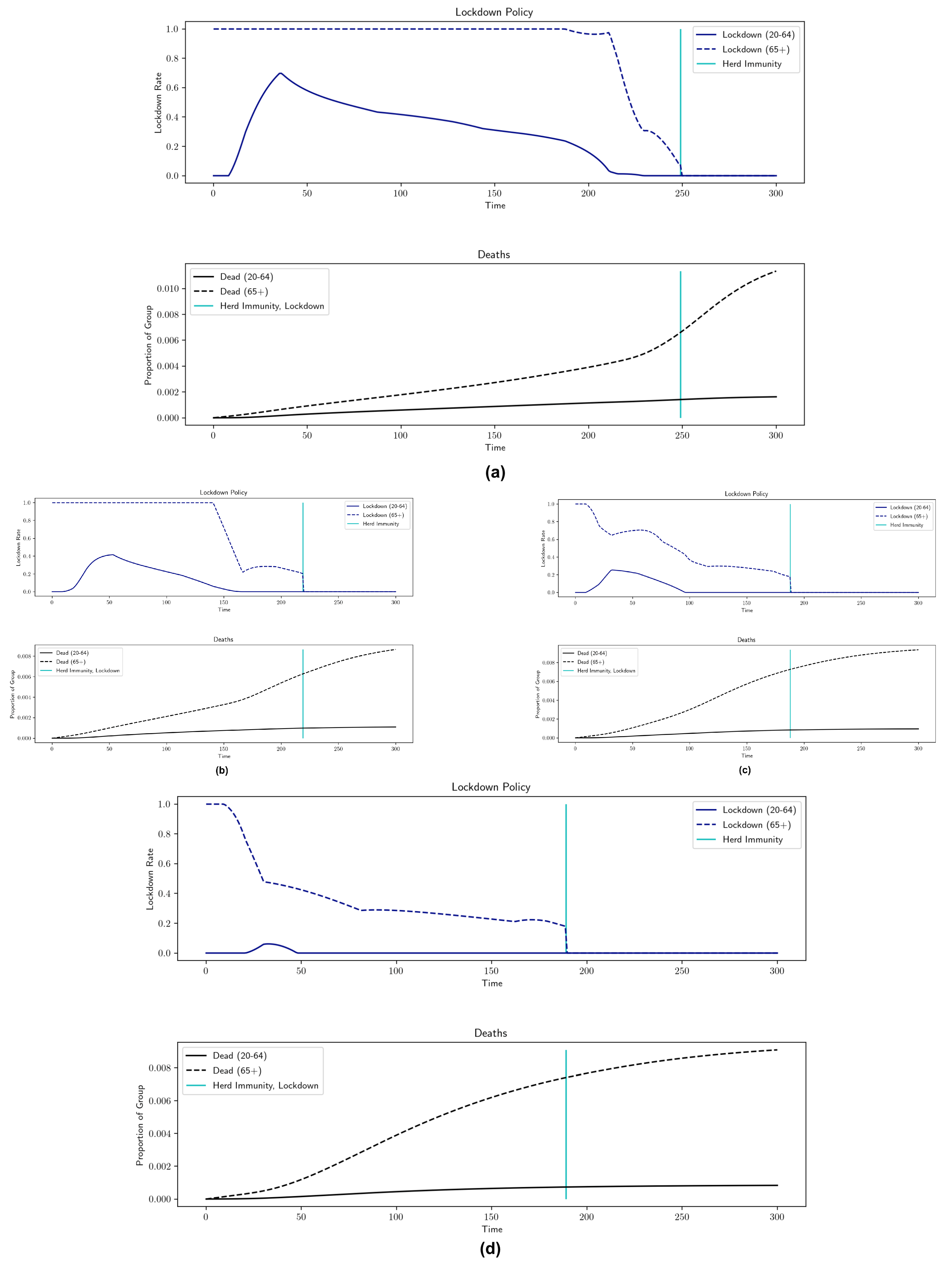
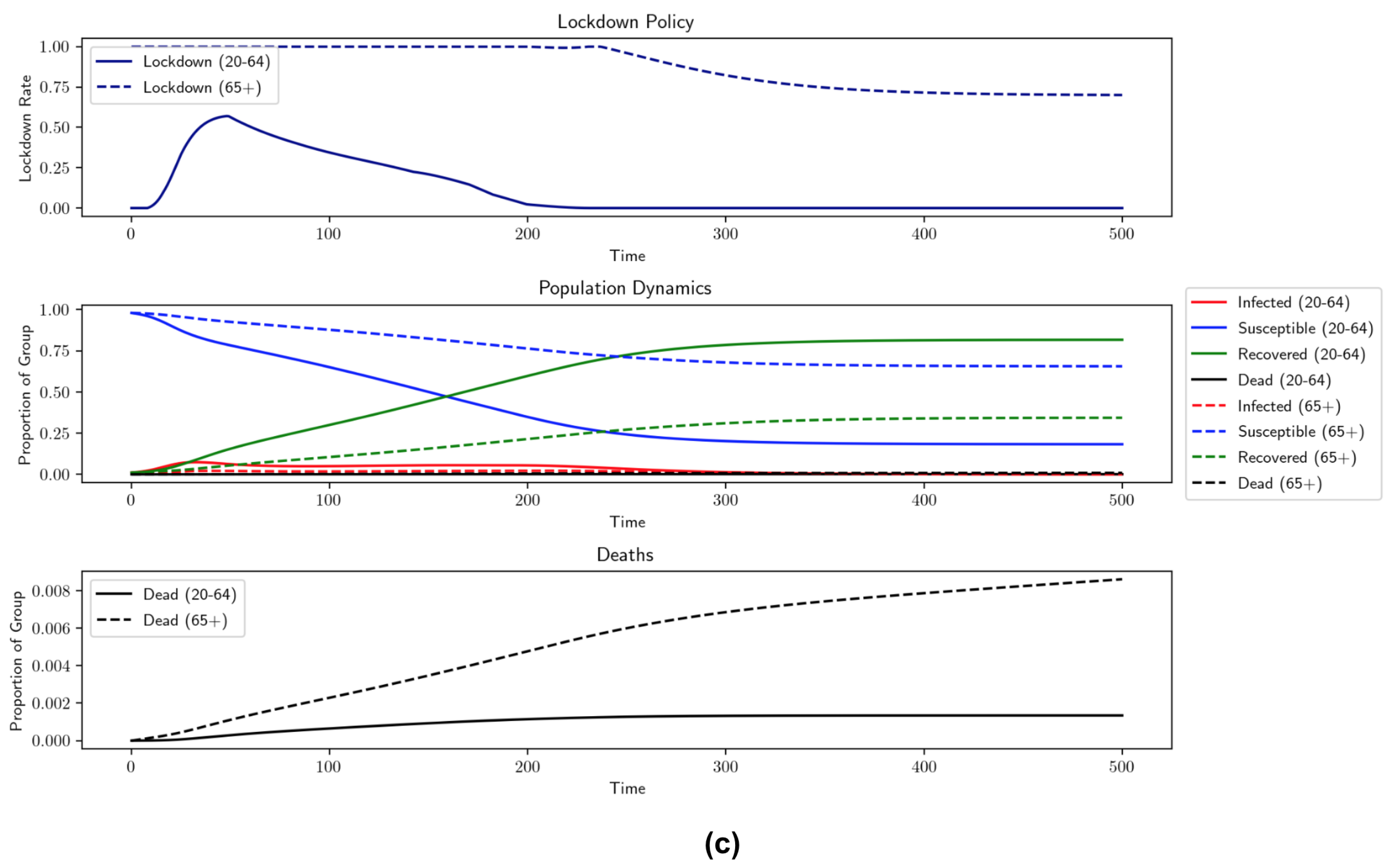
Figure 10.
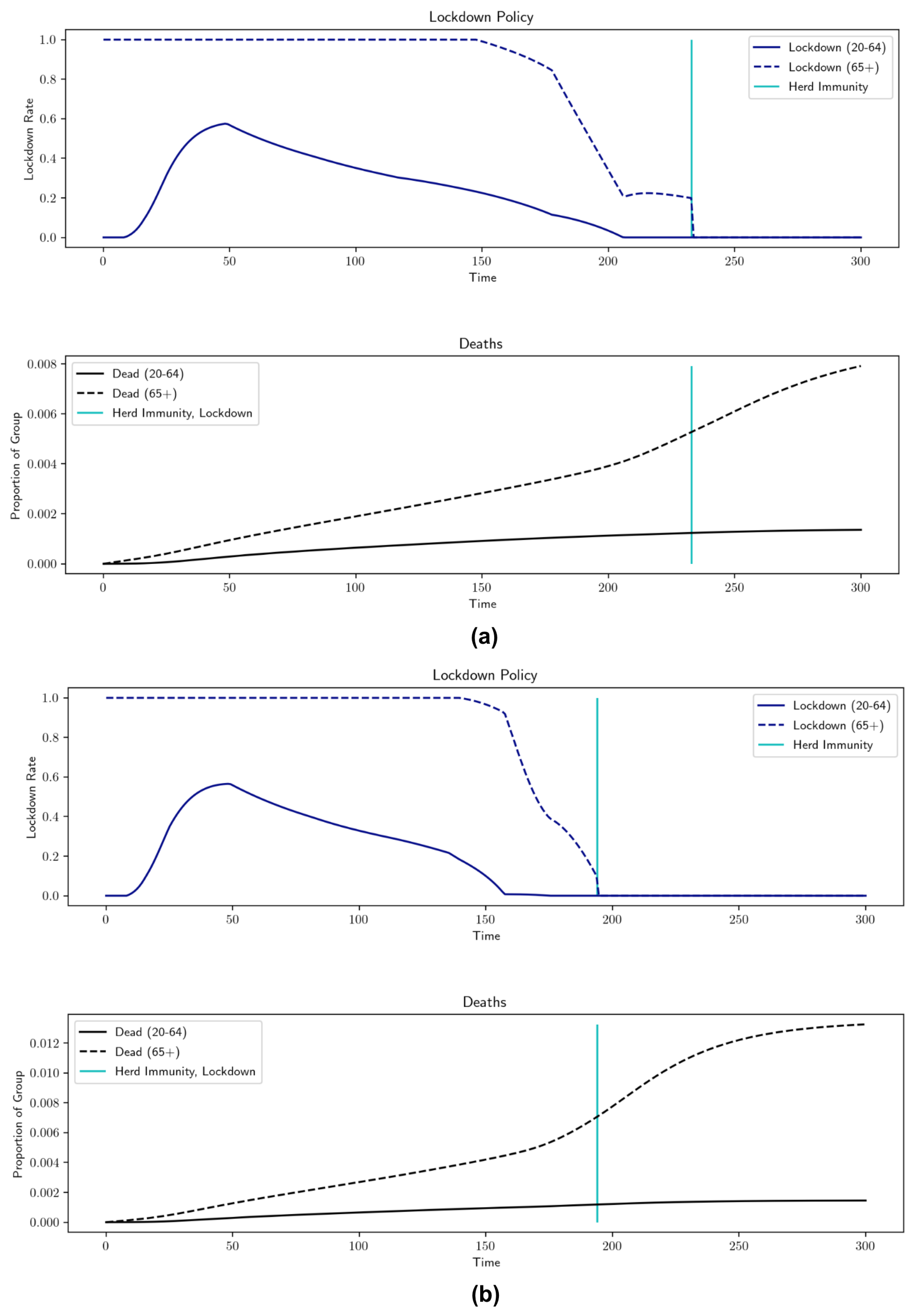
Robustness results for (scale factor for individual carefulness in response to current levels of infection). , , , , , , , , . (a) , lockdown: 249 d, output loss: 10.6699%, total deaths: 0.3712%; (b) , lockdown: 219 d, output loss: 4.5236%, total deaths: 0.2651%; (c) , lockdown: 188 d, output loss: 1.9019%, total deaths: 0.259%; (d) , lockdown: 189 d, output loss = 0.1558%, total deaths = 0.245%.
Figure 10.
Robustness results for (scale factor for individual carefulness in response to current levels of infection). , , , , , , , , . (a) , lockdown: 249 d, output loss: 10.6699%, total deaths: 0.3712%; (b) , lockdown: 219 d, output loss: 4.5236%, total deaths: 0.2651%; (c) , lockdown: 188 d, output loss: 1.9019%, total deaths: 0.259%; (d) , lockdown: 189 d, output loss = 0.1558%, total deaths = 0.245%.

Figure 11.
Robustness results for (arrival of herd immunity). , , , , , , , , , . (a) Herd immunity = 65%, output loss: 7.8084%, total deaths: 0.2948%; (b) herd immunity = 70%, output loss = 7.8496%, total deaths = 0.2724%; (c) herd immunity = 75%, output loss: 7.967%, total deaths: 0.2732%.
Figure 11.
Robustness results for (arrival of herd immunity). , , , , , , , , , . (a) Herd immunity = 65%, output loss: 7.8084%, total deaths: 0.2948%; (b) herd immunity = 70%, output loss = 7.8496%, total deaths = 0.2724%; (c) herd immunity = 75%, output loss: 7.967%, total deaths: 0.2732%.


| Group | ||
|---|---|---|
| Age 20–64 | ||
| Age 65+ |
Table 2.
Comparison of the optimal lockdown policy to no lockdown, using benchmark parameters.
| Situation | Output Loss | Total Deaths |
|---|---|---|
| No Lockdown | 0% | 0.6189% |
| Optimal Lockdown | 7.3439% | 0.3266% |
Table 3.
A comparison of mortality rates for different nonpecuniary values of life; death rates from Table 1.
Table 3.
A comparison of mortality rates for different nonpecuniary values of life; death rates from Table 1.
| Nonpecuniary Value of Life | Output Loss | Total Deaths (All) | COVID-19 Deaths (All) | Total Deaths (20–64) | COVID-19 Deaths (20–64) | Total Deaths (65+) | COVID-19 Deaths (65+) |
|---|---|---|---|---|---|---|---|
| 0% | 0.4464% | 0.4335 % | 0.1433% | 0.1433% | 0.3017% | 0.2902% | |
| (Benchmark) | 7.3439% | 0.3266% | 0.2544% | 0.1201% | 0.0855% | 0.2066% | 0.1689% |
Table 4.
Parameter robustness results (note: lockdown for 65+ ends at herd immunity). Benchmark parameters: , , , , , , , , , , . Death rates from Table 1. herd immunity threshold = 60%.
Table 4.
Parameter robustness results (note: lockdown for 65+ ends at herd immunity). Benchmark parameters: , , , , , , , , , , . Death rates from Table 1. herd immunity threshold = 60%.
| Parameter Values | Avg. Lockdown (20–64) | Length (20–64) (Days) | Avg. Lockdown (65+) | Length (65+) (Days) | Output Loss (%) | Total Deaths (%) | COVID-19 Deaths (%) |
|---|---|---|---|---|---|---|---|
| Benchmark | 0.3188 | 161 | 0.8819 | 207 | 7.3439 | 0.3266 | 0.2544 |
| 0.3123 | 205 | 0.8878 | 239 | 8.9667 | 0.3265 | 0.2388 | |
| 0.2864 | 126 | 0.8663 | 167 | 5.2962 | 0.338 | 0.2848 | |
| 0.3083 | 192 | 0.8863 | 227 | 8.3612 | 0.2456 | 0.2456 | |
| 0.2689 | 116 | 0.8511 | 154 | 4.6199 | 0.5319 | 0.2977 | |
| 0.3582 | 214 | 0.9057 | 249 | 10.6699 | 0.3712 | 0.2707 | |
| 0.2173 | 144 | 0.7758 | 219 | 4.5236 | 0.2651 | 0.2106 | |
| 0.1503 | 84 | 0.4962 | 188 | 1.9019 | 0.259 | 0.2328 | |
| 0.041 | 24 | 0.3852 | 189 | 0.1558 | 0.245 | 0.2314 | |
| 0.2874 | 126 | 0.8631 | 168 | 8.8592 | 0.338 | 0.2846 | |
| 0.3106 | 201 | 0.8866 | 235 | 5.842 | 0.3251 | 0.2394 | |
| 0.2989 | 193 | 0.8418 | 233 | 8.118 | 0.2753 | 0.1955 | |
| 0.3316 | 147 | 0.891 | 194 | 7.0292 | 0.3657 | 0.2975 | |
| 0.3065 | 175 | 0.855 | 211 | 7.6457 | 0.3324 | 0.2588 | |
| 0.3177 | 160 | 0.8803 | 206 | 6.8007 | 0.3264 | 0.2548 | |
| 0.3171 | 158 | 0.88 | 204 | 6.0805 | 0.3262 | 0.2556 | |
| 0.3188 | 161 | 0.8819 | 207 | 7.3439 | 0.3266 | 0.2544 | |
| 0.3188 | 161 | 0.8819 | 207 | 7.3439 | 0.3266 | 0.2544 | |
| 0.3552 | 129 | 0.8792 | 161 | 6.7354 | 0.3589 | 0.2992 | |
| 0.2736 | 266 | 0.8815 | 304 | 9.7995 | 0.3075 | 0.2023 | |
| 0.2982 | 185 | 0.8973 | 242 | 7.8084 | 0.2948 | 0.2135 | |
| 0.2983 | 186 | 0.8919 | 279 | 7.8496 | 0.2724 | 0.1852 | |
| 0.2793 | 202 | 0.8633 | Vaccine | 7.967 | 0.2732 | 0.1444 | |
| 0.2775 | 204 | 0.9909 | Vaccine | 7.9881 | 0.2834 | 0.1416 | |
| 0.2754 | 206 | 1.0 | Vaccine | 8.0011 | 0.2832 | 0.1405 | |
| 0.2754 | 206 | 1.0 | Vaccine | 8.0011 | 0.2832 | 0.1405 |
Publisher’s Note: MDPI stays neutral with regard to jurisdictional claims in published maps and institutional affiliations. |
© 2021 by the authors. Licensee MDPI, Basel, Switzerland. This article is an open access article distributed under the terms and conditions of the Creative Commons Attribution (CC BY) license (https://creativecommons.org/licenses/by/4.0/).
Share and Cite
MDPI and ACS Style
Bayraktar, E.; Cohen, A.; Nellis, A. A Macroeconomic SIR Model for COVID-19. Mathematics 2021, 9, 1901. https://doi.org/10.3390/math9161901
AMA Style
Bayraktar E, Cohen A, Nellis A. A Macroeconomic SIR Model for COVID-19. Mathematics. 2021; 9(16):1901. https://doi.org/10.3390/math9161901
Chicago/Turabian StyleBayraktar, Erhan, Asaf Cohen, and April Nellis. 2021. "A Macroeconomic SIR Model for COVID-19" Mathematics 9, no. 16: 1901. https://doi.org/10.3390/math9161901
Note that from the first issue of 2016, this journal uses article numbers instead of page numbers. See further details here.