
Assessing the Impact of the COVID-19 Shock on a Stochastic Multi-Population Mortality Model


1
Faculty of Economics and Business, KU Leuven, 3000 Leuven, Belgium
2
Faculty of Economics and Business, University of Amsterdam, 1012 WX Amsterdam, The Netherlands
*
Author to whom correspondence should be addressed.
Risks 2022, 10(2), 26; https://doi.org/10.3390/risks10020026
Submission received: 9 November 2021
/
Revised: 17 January 2022
/
Accepted: 18 January 2022
/
Published: 21 January 2022
(This article belongs to the Special Issue Impact of the Coronavirus Crisis on Insurance and Financial Mathematics and Risk Analysis)
Abstract
:We aim to assess the impact of a pandemic data point on the calibration of a stochastic multi-population mortality projection model and its resulting projections for future mortality rates. Throughout the paper, we put focus on the Li and Lee mortality model, which has become a standard for projecting mortality in Belgium and the Netherlands. We calibrate this mortality model on annual death counts and exposures at the level of individual ages. This type of mortality data are typically collected, produced and reported with a significant delay of—for some countries—several years on a platform such as the Human Mortality Database. To enable a timely evaluation of the impact of a pandemic data point, we have to rely on other data sources (e.g., the Short-Term Mortality Fluctuations Data series) that swiftly publish weekly mortality data collected in age buckets. To be compliant with the design and calibration strategy of the Li and Lee model, we transform the weekly mortality data collected in age buckets to yearly, age-specific observations. Therefore, our paper constructs a protocol to ungroup the death counts and exposures registered in age buckets to individual ages. To evaluate the impact of a pandemic shock, like COVID-19 in the year 2020, we weigh this data point in either the calibration or projection step. Obviously, the more weight we place on this data point, the more impact we observe on future estimated mortality rates and life expectancies. Our paper allows for quantifying this impact and provides actuaries and actuarial associations with a framework to generate scenarios of future mortality under various assessments of the pandemic data point.
1. Introduction
In December 2019, the coronavirus disease (COVID-19) originated in the Chinese city Wuhan. In the months that followed, the virus spread across the world. At the time of writing, about 87 million positive cases and 1,547,643 deaths have been identified in Europe.1 The United Kingdom has the highest absolute number of reported COVID-19 deaths in Europe (146,896), followed by Italy (134,831) and France (121,416). Belgium has reported 27,504 deaths.2 The announcements and roll-out of the four COVID-19 vaccines approved by the European Medicine Agency (i.e., from BioNTech and Pfizer, Moderna, AstraZeneca and Johnson & Johnson3) have led to a sharp decline in the number of COVID-19 deaths in Europe. We aim to outline the impact of the COVID-19 pandemic on a stochastic multi-population mortality projection model, such as IA∣BE 2020 published by the Institute of Actuaries in Belgium (Antonio et al. 2020) and AG2020 by the Royal Dutch Actuarial Association (Koninklijk Actuarieel Genootschap 2020). Furthermore, we assess the impact of the pandemic on scenarios generated for future mortality rates with such multi-population mortality models.
The COVID-19 pandemic has impacted mortality in multiple ways. The disease itself has led to an increase in the number of deaths, especially at the higher ages. However, measures taken by the governments worldwide also impacted mortality in a positive way, leading to less traffic or work-related accidents in 2020 and an increased awareness of sanitary precautions leading to a mild flu season in the winter of 2020–2021. Vanella et al. (2021) assess the excess mortality during the COVID-19 pandemic with a novel approach inspired by principal component analysis. While this paper puts focus on the mortality projection standard for the Belgian population, as documented in IA∣BE 2020, we acknowledge some other, recent contributions that aim at assessing the impact of COVID-19 on mortality forecasts. Koninklijk Actuarieel Genootschap (2020) performs a sensitivity analysis that shows the impact of the pandemic on the Dutch cohort life expectancies in 2021 by feeding virtual deaths and exposures in 2019–2020 to the AG2020 model. van Delft and Huijzer (2020) use Koninklijk Actuarieel Genootschap (2018) as a starting point and investigate the impact of four different COVID-19 scenarios on the Dutch best estimate mortality table published in 2018. They create these COVID-19 scenarios by multiplying the mortality rates in 2020 (and later) with a shock factor. These shocks are defined for a particular age bucket as (a fraction of) the ratio of the observed death rate in the first 23 weeks of 2020 to the average of the observed death rates in the first 23 weeks in earlier years. Next, the Continuous Mortality Investigations (CMI) in the UK provide regular updates on the excess of deaths and mortality in the United Kingdom due to COVID-19.4 In their updates (CMI working papers 137, 143, 147), the calibration process of the CMI_2020 mortality model is adjusted to enable the weighting of observations. In the core version of CMI_2020, a weight of zero is attached to the 2020 data point and a weight of to all other years. The CMI working papers 157 and 159 sketch ideas for the CMI_2021 mortality model and intend to give the 2020 and 2021 data points both a weight of zero.
As outlined in Antonio et al. (2020), IA∣BE 2020 calibrates a mortality model of type Li and Lee (Li and Lee 2005) on the data set with the annual observed number of deaths, , and the corresponding exposures to risk, , registered at individual ages. More specifically, IA∣BE 2020 puts focus on a set of countries over the calibration period 1988–2018 (European trend) and 1988–2019 (Belgian trend) with age range 0–90. While data collected in age buckets are swiftly available from the Short-Term Mortality Fluctuations ([STMF]) Data series or Eurostat, the publication of individual age statistics takes more time. Therefore, we propose a protocol to move from weekly mortality data registered in age buckets to annual mortality data at individual ages. This is a first contribution of our paper to the existing literature on mortality modelling. Rizzi et al. (2015) use the composite link model to ungroup coarsely grouped data, but their underlying smoothness assumption would lead to a smooth exposure and death curve. However, our protocol attempts to capture the age-specific pattern within such curves, based on historically observed data. We use our protocol to create (virtual) exposures and deaths at individual ages for the year 2020 (or earlier if necessary), leading to an extended multi-population mortality data set until the year 2020 on an individual age basis. In this paper, we then assess the impact of COVID-19 on the calibration of and projections with a stochastic multi-population mortality model using this extended data set. Related work is in Schnürch et al. (2021), who investigate the impact of COVID-19 on the parameters, forecasts and implied present values of life contingent liabilities with the simple Lee and Carter mortality model (Lee and Carter 1992) using mortality data collected in age buckets. Our work extends the current literature by focusing on a multi-population instead of a single population mortality model, calibrated on data collected at individual ages. Moreover, we investigate the COVID-19 impact on future mortality rates and life expectancies by proposing ways to weigh the impact of this pandemic data point in either the calibration or projection set-up.
This paper is organised as follows: first, Section 2 introduces some basic concepts and discusses notation. Moreover, we list the data sources that provide us with weekly and annual death counts and exposures at the level of individual ages or age buckets. In Section 3, we then introduce the model specifications, the assumed time dynamics and the calibration and projection methodology of the stochastic multi-population mortality projection model used in Antonio et al. (2020) and Koninklijk Actuarieel Genootschap (2020). In addition, we specify the multi-population data set and the calibration period in the mortality model for Belgium. In Section 4, we create the COVID-19 impacted data set of deaths and exposures until the year 2020 by ungrouping the data collected in age buckets to data at the level of individual ages. Next, we recalibrate the multi-population mortality model underlying the IA∣BE 2020 framework and present different methods to deal with the 2020 pandemic data point in Section 5. We also assess the impact of COVID-19 on the cohort life expectancy in 2020 using the different weighting scenarios for the pandemic data point. Section 6 provides a literature review of some alternative techniques to deal with mortality shocks in the modelling process of a stochastic mortality model of type Lee and Carter. We conclude in Section 7. Technical details are deferred to the Appendix. We list the data sources in Appendix A. Appendix B describes the construction of the virtual exposure points for ages 0–90 and years 2019–2020. In Appendix C, we construct the death counts for the same set of ages and years. Appendix D then validates the proposed protocols from Appendix B and Appendix C by comparing the virtual exposures and deaths in the year 2020 with the actual observations for Belgium and Denmark.
2. Data and Notation
Basic concepts.
Let denote the mortality rate at exact age x in year t. This mortality rate refers to the probability that an x year old person who was born on 1 January of year and is still alive at 1 January of year t dies within the next year. In addition, let denote the force of mortality, i.e., the instantaneous rate of mortality at exact age x in year t. We assume that the force of mortality is constant in between exact ages and years, i.e., for . Under this piecewise constant force of mortality assumption, we obtain
Stochastic mortality models, as mentioned in Section 1, often model a transformation of the force of mortality or the mortality rate .
Data sources: annually, at individual ages.
Li and Lee’s stochastic multi-population mortality projection model (Li and Lee 2005), as considered in this paper, models the logarithm of using mortality data on a collection of European countries. Hereto, mortality data are collected over a certain calibration period and a range of ages . We use annual mortality data consisting of the observed number of deaths and the observed exposures to risk , as available from sources like the Human Mortality Database ([HMD])5, Eurostat6 or an official national statistics institute like Statbel in Belgium.7 The latter data source is typically used to extract the most recent mortality information from the country of interest, in our case Belgium.
Data sources: weekly, in age buckets.
The data sources discussed above typically report annual mortality statistics at the individual age level with a significant delay (for some countries with a delay of several years). To evaluate the impact of a pandemic shock on a mortality projection model, we therefore need other data sources that report mortality statistics in a more timely manner. Hereto, we consult the Short-Term Mortality Fluctuations ([STMF]) Data series8 and Eurostat.9 With only a minor delay of a few weeks, they provide weekly mortality data registered in age buckets rather than at the individual age level. To be compliant with the design of a stochastic multi-population mortality model, Section 4 outlines a protocol to transform these weekly mortality statistics in age buckets into annual death counts and exposures at individual ages. We use the following notations (for now, we leave out gender g in our notation):
for the death counts, exposures and (central) death rates in age bucket in week w in year t, respectively. Here, the week .10 We now further explain the weekly mortality information retrieved from the STMF data series and Eurostat:
STMF. The STMF data series reports death counts and death rates in age buckets. The weekly death rates are derived from the weekly death counts and exposures using the following relationship:
The STMF data series reports the weekly mortality statistics in large age buckets:
The exposures , used to calculate the death rates in Equation (1), are based on the observed annual exposures registered at individual ages, as reported by the HMD. However, for the most recent years, the exposures are not available yet and estimates have to be made. The STMF data series documentation explains the construction of these unknown exposures at the level of individual ages.11 In addition, the STMF data series assumes a constant weekly exposure per year, per age bucket and per gender. The weekly exposure , as reported in the STMF data series in age buckets, is the yearly (estimated) exposure divided by 52 and aggregated over the individual ages in the age bucket .
Eurostat. Next to the HMD and its STMF data series project, Eurostat lists valuable data sets related to death counts, useful to assess the impact of COVID-19 on mortality rates. Eurostat does not report any information about weekly exposures. From Eurostat, we obtain the death counts by week, gender and 5-year age bucket.12 The 19 respective age buckets are
For many countries, the STMF reported death counts correspond to the aggregated death counts reported by Eurostat. If this correspondence holds true, the data from Eurostat is more preferable due to the smaller age buckets, which eventually leads to a more accurate transition towards death counts at individual ages, necessary in the stochastic multi-population mortality projection model. For data quality reasons, we only use the Eurostat reported weekly death counts in the small age buckets whenever their aggregated death counts correspond to the ones reported in the STMF data series. This is the case for all countries, except Germany13, France and the United Kingdom.
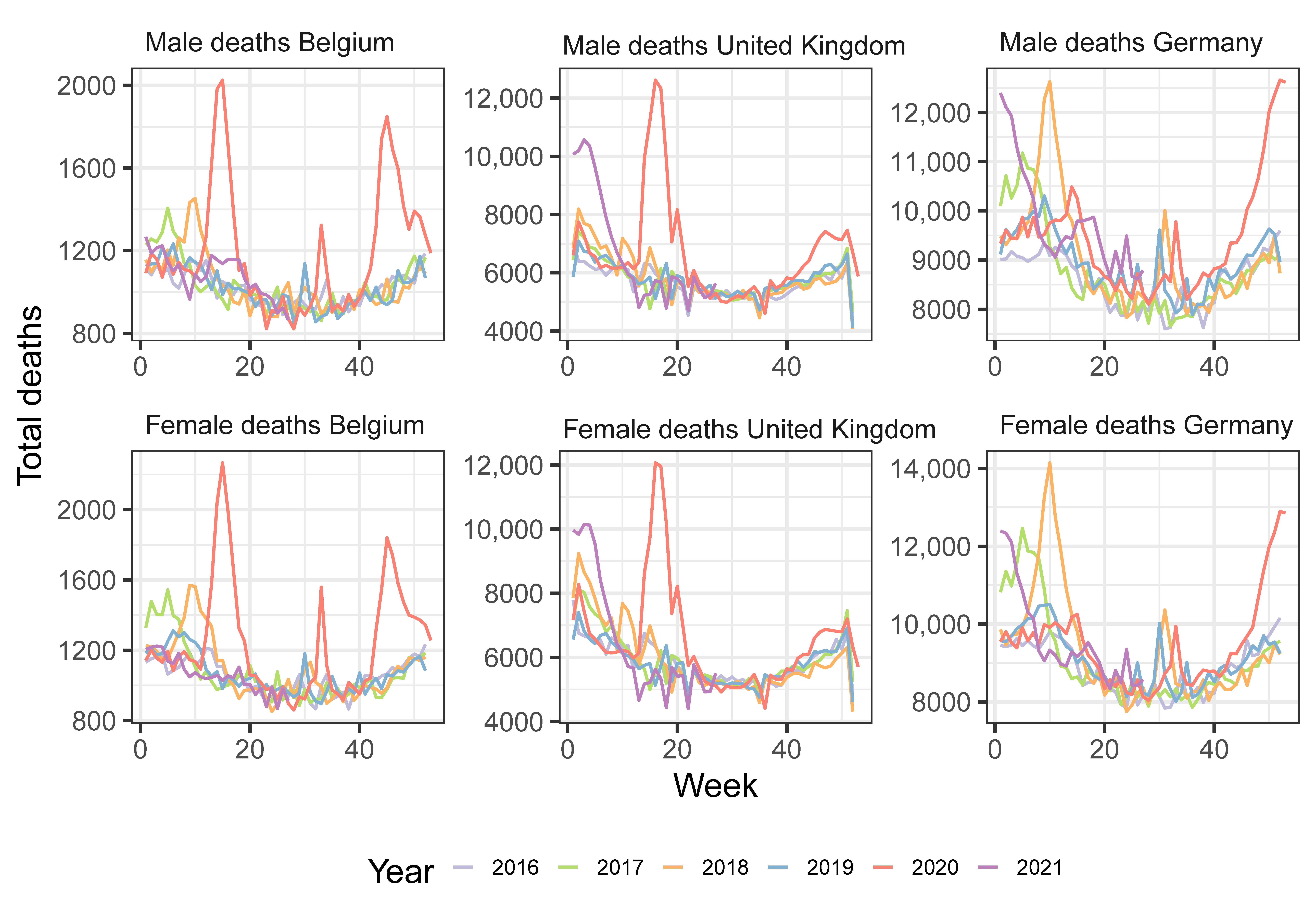
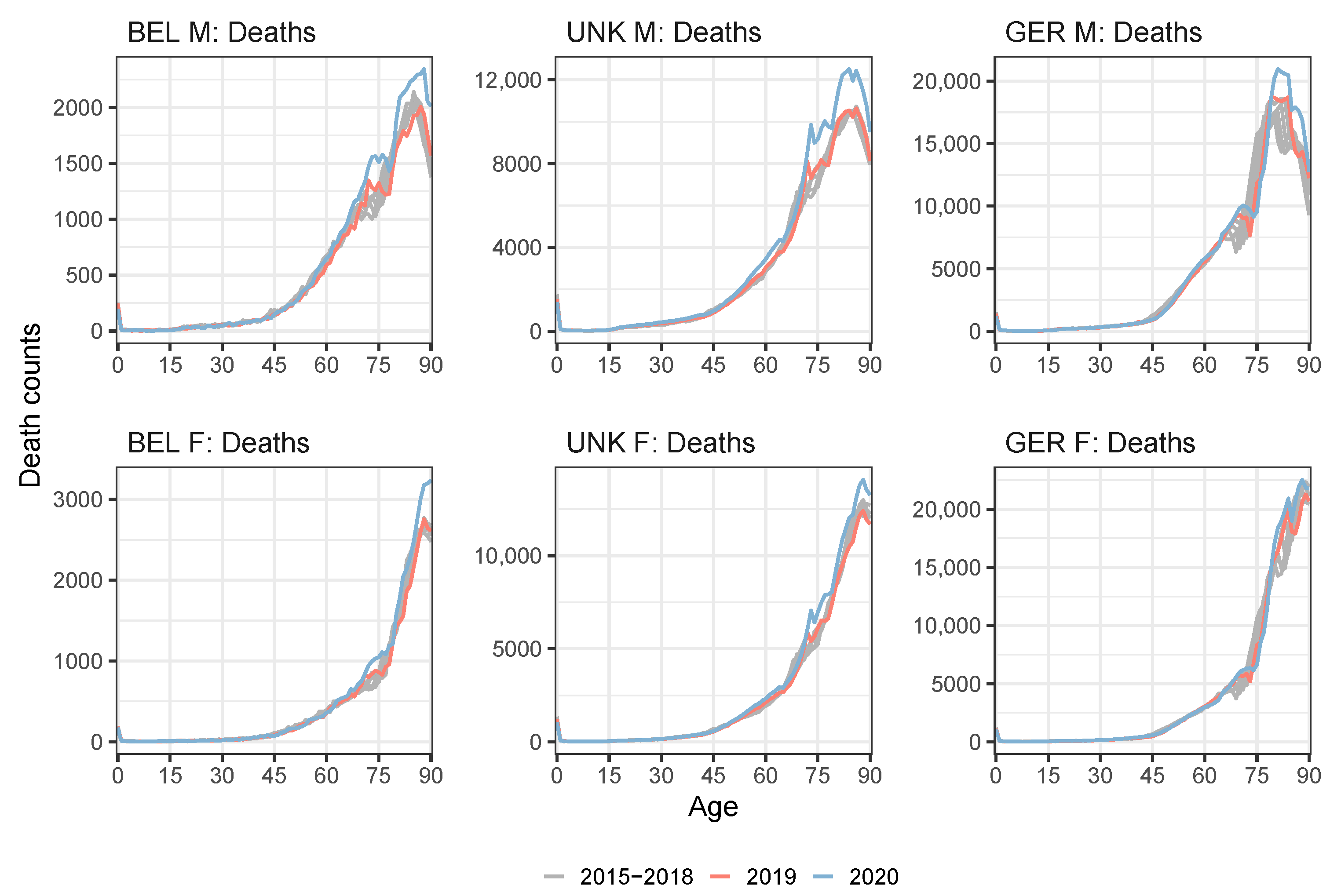
Figure 1 illustrates the number of deaths per week for the years 2016–2021 for Belgium, United Kingdom and Germany. We clearly observe (multiple) peaks corresponding to various COVID-19 waves.
3. A Stochastic Multi-Population Mortality Standard of Type Li and Lee
Antonio et al. (2017) provide an in-depth discussion motivating the use of the Li and Lee model as a mortality projection standard for the Dutch and Belgian population. This motivation is threefold. First, a stochastic projection model is preferred thanks to its ability to quantify the uncertainty in mortality and life expectancy forecasts and to generate scenarios of future mortality. Second, by combining country-specific data with data from other, similar European countries, the multi-population approach is more robust compared to the single population strategy. Third, the choice for the Li and Lee model is based on an extensive, comparative analysis of the various mortality models discussed in Cairns et al. (2009), Haberman and Renshaw (2011), Börger et al. (2014), Van Berkum et al. (2016) and Haberman et al. (2014). Models in this comparative analysis have been compared in terms of statistical criteria (in- and out-of-sample) and biological reasonableness. The goal of this paper is to evaluate the impact of a pandemic shock on mortality forecasts from this model of type Li and Lee. The tools and methods to achieve this, as we develop in Section 5, can be generalized to other types of mortality models.
3.1. The Li and Lee Mortality Model
Specification.
The Li and Lee mortality model (Li and Lee 2005) structures the logarithm of the force of mortality for a country of interest c as:
We recognize two Lee and Carter specifications (Lee and Carter 1992), one to model a common mortality trend (driven by ) and one to model the country-specific deviation from this common trend (driven by ). This common trend reflects the global mortality trend over a collection of countries. We impose two sets of parameter constraints to avoid identification problems:
We deviate from the usual Lee and Carter constraints, i.e., , to achieve better numerical stability in the calibration process, as motivated in Antonio et al. (2015).
Calibration.
We calibrate the mortality model in Equation (2) on annual data with the observed number of deaths, , and the exposures to risk, , over a specified age range and over a specified calibration period . We hereby impose a Poisson distribution on the number of deaths random variable (Brouhns et al. 2002) and apply a conditional maximum likelihood approach (Li 2013). We perform the calibration of the Li and Lee mortality model in Equation (2) separately on male (M) and female (F) mortality data. This will result in calibrated Li and Lee parameters and for . We do not emphasize the dependence on g for notational convenience.
- 1.
- In a first step, we calibrate the parameters , and in the common mortality trend by assuming that the total number of deaths random variable follows a Poisson distribution with mean . Hereto, we maximize the following Poisson log-likelihood:where and are the observed number of deaths and exposures, respectively, aggregated over the collection of countries. Furthermore, . In this first calibration step, we impose the constraints in Equation (3) on and .
- 2.
- In a second step, we calibrate the country-specific parameters and by assuming that the number of deaths random variable , in the country of interest c, follows a Poisson distribution with mean . Hereto, we maximize the Poisson log-likelihood, conditional on the estimates obtained in step 1:where and are the observed number of deaths and exposures in country c, respectively. Furthermore, we have . In this second calibration step, we impose the Lee and Carter constraints in Equation (3) on and .
3.2. The Time Dynamics
Specification.
We model the time dynamics of the common period effect, i.e., , and the country-specific period effect, i.e., , for males and females separately. Based on the discussion in Li and Lee (2005) and on the work of Antonio et al. (2020) and Koninklijk Actuarieel Genootschap (2020), we model by a Random Walk with Drift ([RWD]) and the country-specific period effect, , with an AR(1) model. An AR(1) parameter lower than one then ensures that the country-specific mortality trend does not diverge from the common mortality trend in the long run. We denote:
We can then express the four-dimensional vector of time series for as:
The four-dimensional vectors of noise terms are independent over time and follow a four-dimensional Gaussian distribution with mean and covariance matrix .
Calibration.
Let be the unknown parameter vector, collecting the parameters used in and as well as in the covariance matrix . Inspired by Koninklijk Actuarieel Genootschap (2020), we estimate on the calibrated and parameters jointly for males and females by maximizing the four-dimensional Gaussian log-likelihood:14
Forecasting.
We now use these calibrated time dynamics to generate future paths for the country-specific mortality rates . We consider a projection period . Hereto, we start from the calibrated period effects in the last year of the calibration period , i.e., (, , , ). We then take random draws for and from the fitted Gaussian distribution with mean and covariance matrix . We obtain future paths of the calibrated period effects for males and females using Equation (4). Note that we generate future paths starting from and for all i and each gender g. We obtain a best-estimate forecast for the calibrated period effects by taking the zero vector for the noise terms in Equation (4), i.e., using for .
3.3. Generating Future Paths of Mortality Rates and Life Expectancies
Mortality rates.
Using Equation (2) and the calibrated Li and Lee parameters and , we can now generate future paths for the country-specific mortality rates. Let us denote and for the i-th generated value of the country-specific mortality rate and the country-specific force of mortality respectively. Then, we obtain:
with , and . Having obtained a scenario for the mortality rates for ages 0–90 in a future year, we close the generated mortality rates until age 120 using the method of Kannisto (1994). We refer to Antonio et al. (2020) for a detailed explanation of this method.
Life expectancy.
We obtain future paths of the period and cohort life expectancies of an x year old in year t (Pitacco et al. 2009) as:
We obtain best-estimate forecasts for the mortality rates and the period and cohort life expectancies by using the best-estimate forecasts of the calibrated period effects .
3.4. The Li and Lee Mortality Model for the Belgian Population
IA∣BE 2020 is based on a mortality model of type Li and Lee and puts focus on Belgium as the country of interest (). The common trend in Equation (2) is a European mortality trend calibrated on a set of countries with a Gross Domestic Product per capita above the European average in 2018.15 As such, the multi-population data set combines mortality data from Belgium, The Netherlands, Luxembourg, Norway, Switzerland, Austria, Ireland, Sweden, Denmark, Germany, Finland, Iceland, United Kingdom and France. Furthermore, IA∣BE 2020 calibrates the mortality model on annual data registered at the level of individual ages, from the HMD, Eurostat and the Belgian statistical institute Statbel. IA∣BE 2020 calibrates the parameters in the European mortality trend on a range of years 1988–2018 and the Belgium-specific mortality trend on the range of years 1988–2019.
The aim of this paper is to recalibrate the Li and Lee mortality model on a multi-population data set consisting of the same set of countries, but on a calibration period from 1988 to 2020. Hereto, we use the STMF data series and Eurostat, providing weekly mortality statistics collected in age buckets. Neither the STMF data series nor Eurostat report granular mortality information on Ireland. While Ireland is part of the set of countries defined in IA∣BE 2020 to calibrate the common European mortality trend, we exclude this country in the COVID-19 impact assessment covered in this paper. However, given the exposure size of the Irish population, we do not expect that this has a major impact on the results obtained with the multi-population mortality model.
4. Transforming Weekly Mortality Data in Age Buckets to Annual Mortality Data at Individual Ages
Our strategy to evaluate the impact of COVID-19 on a stochastic multi-population mortality projection model of type Li and Lee adheres to the design principles of the model. Therefore, we refrain from calibrating the multi-population model directly to a mortality data set registered in age buckets, but make the transition to a data set at the level of individual ages. In addition, this transition will facilitate a comparison between the results from Section 5 and the ones from the original IA∣BE 2020 model (Antonio et al. 2020). As explained in Section 3.4, we have to supplement our multi-population data set with mortality data for the most recent years 2019–2020. Hereto, we use the weekly mortality statistics in age buckets, retrieved from the STMF data series and Eurostat. We propose a protocol to make the transition from the weekly deaths and exposures collected in age buckets to the required format. Section 4.1 discusses the transition from weekly to annual deaths and exposures collected in age buckets. In Section 4.2, we convert the annual deaths and exposures to data at the level of individual ages.
4.1. From Weekly to Annual Mortality Data Registered in Age Buckets
STMF.
The Short-Term Mortality Fluctuations Data series, as discussed in Section 2, assume a constant weekly exposure per year, per age bucket and per gender. When going from the weekly exposures available from the STMF data series to annual exposures, we simply multiply the weekly exposures with a factor 52, i.e., the number of weeks in a year:
where now denotes the total annual exposure in year t for age bucket .
STMF and Eurostat.
The weekly mortality data sources, i.e., the STMF data series and Eurostat, follow the definition of `week’ given by the ISO week date system, which is part of the ISO-8601 date and time standard.16 In this system, a year consists of 52 or 53 full weeks. When a year t consists of 53 weeks instead of the usual 52 weeks,17 we adjust the calculation of the yearly death counts to be compliant with the HMD and Eurostat individual death counts:
where and are respectively the fraction of the first and 53rd ISO week that are part of calendar year t. In addition, the STMF data series lists death counts and death rates for Northern Ireland, England and Wales and Scotland separately. A simple aggregation of their death counts leads to the death counts of the United Kingdom as a whole.
4.2. Ungrouping Data from Age Buckets to Individual Ages
We start from the annual deaths and exposures collected in age buckets, as obtained from Section 4.1. We then define a protocol to ungroup the data in age buckets to data at the level of individual ages. Rizzi et al. (2015) introduce a method that ungroups histograms (or coarsely grouped data), using a composite link model with a penalty to ensure the smoothness of the underlying distribution. Their strategy is not able to capture the typical patterns in the evolution of the exposures or death counts over time. As an example, Figures 3 and 5 in this paper clearly show the evolution of certain spikes in the exposure and death curve over time, i.e., the spikes are moving to the right by one age each subsequent year. These observed spikes or patterns within an age bucket cannot be captured by the method of Rizzi et al. (2015). Therefore, we propose an alternative strategy that is capable of picking up these spikes. At the same time, we ensure that the sum of the individual, ungrouped number of deaths and exposures in an age bucket corresponds to the exposures and deaths in that age bucket, reported in the STMF data series or by Eurostat. We call the newly created annual deaths and exposures at the level of individual ages, virtual deaths and exposures.
Protocol to ungroup .
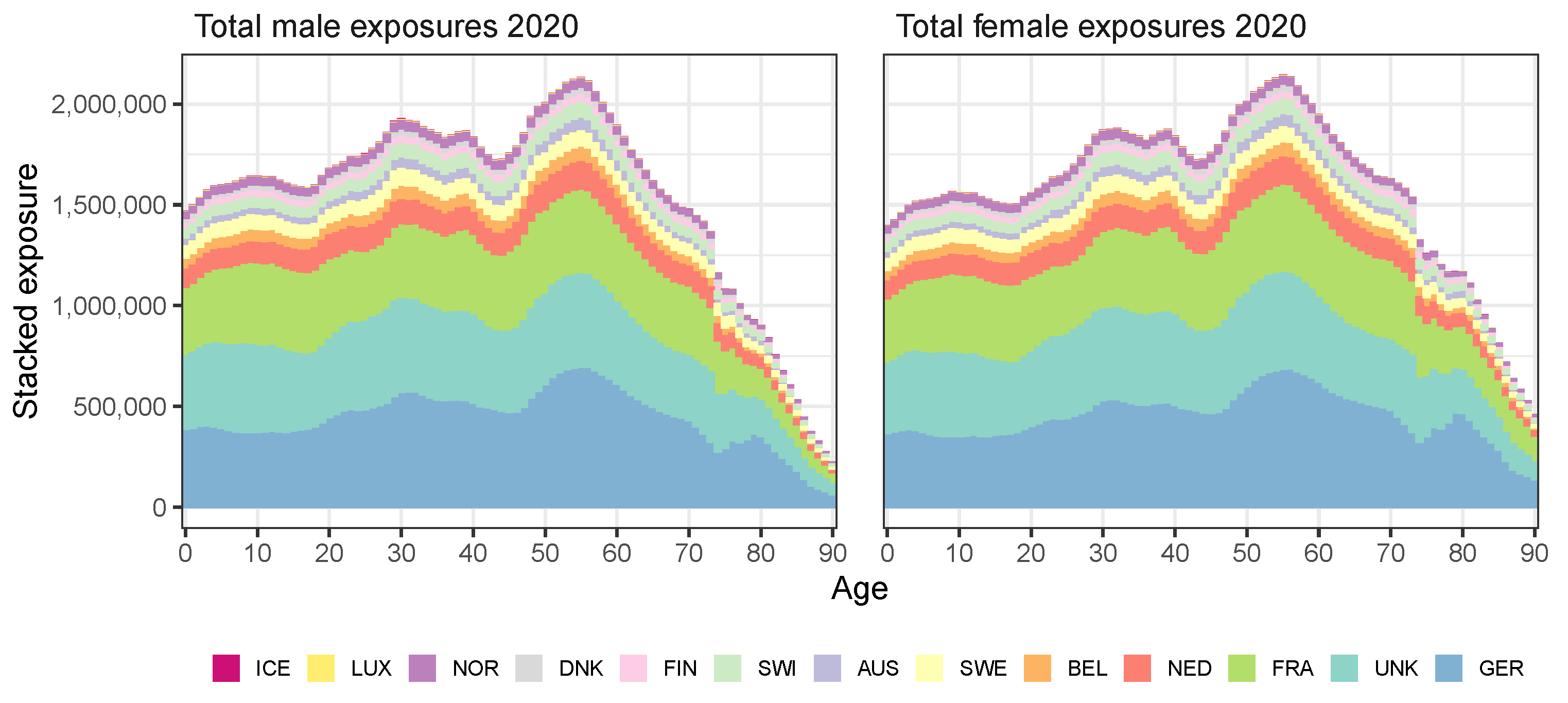
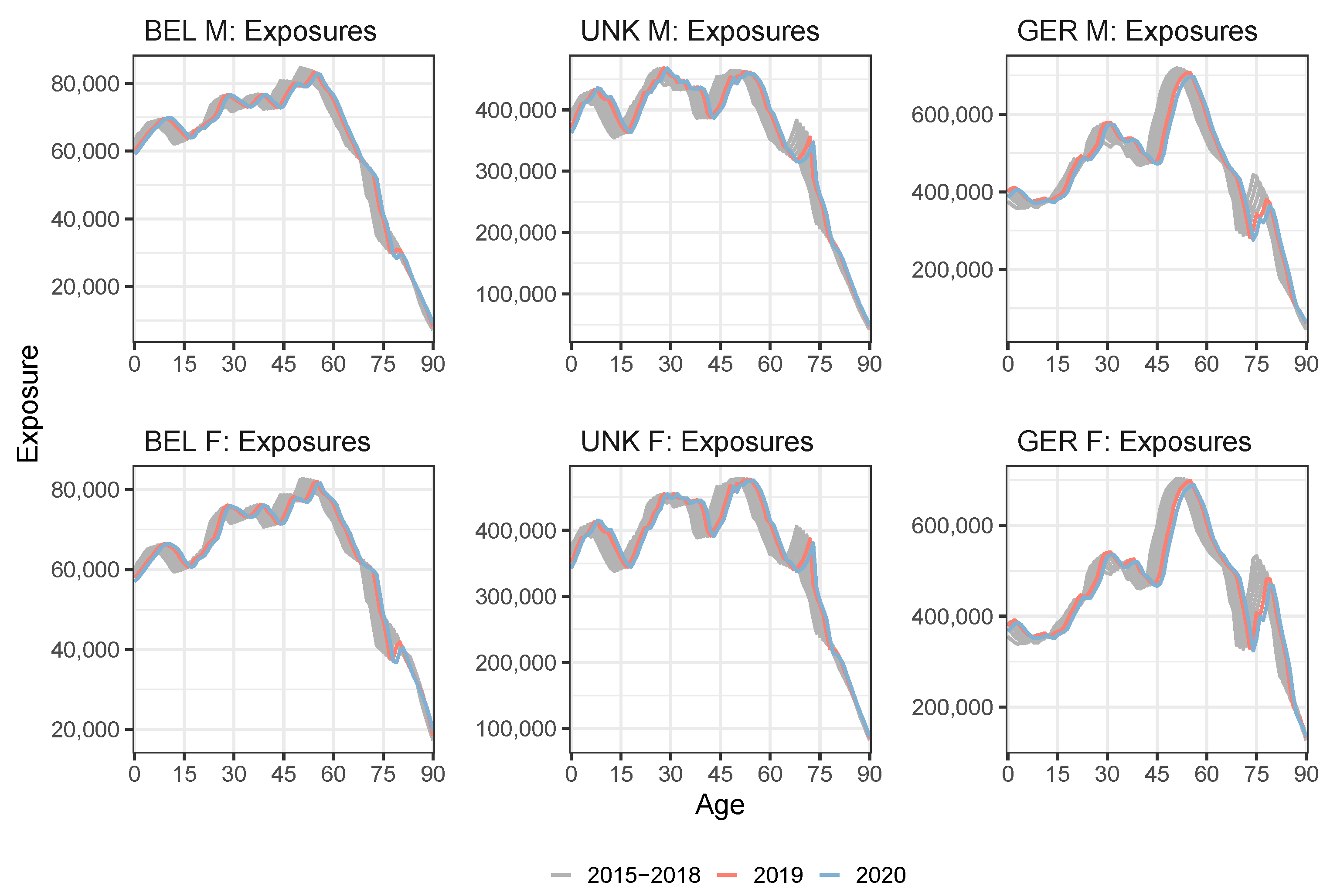
To obtain annual exposures at individual ages in an unknown year t, we take the STMF or Eurostat exposure data for the corresponding age buckets. We then allocate these exposures to exposures at individual ages by applying a piecewise scaling of the known exposure curve from a previous year. Appendix B explains our approach in full detail. Figure 2 visualizes the stacked exposures at ages 0–90 in the year 2020 for all 13 European countries under consideration for males (left) and females (right). Figure 3 shows the evolution of the (virtual) annual exposures for Belgium, the United Kingdom and Germany. The exposures in the year 2020 (and 2019 for the United Kingdom) are created using our approach.
Protocol to ungroup .
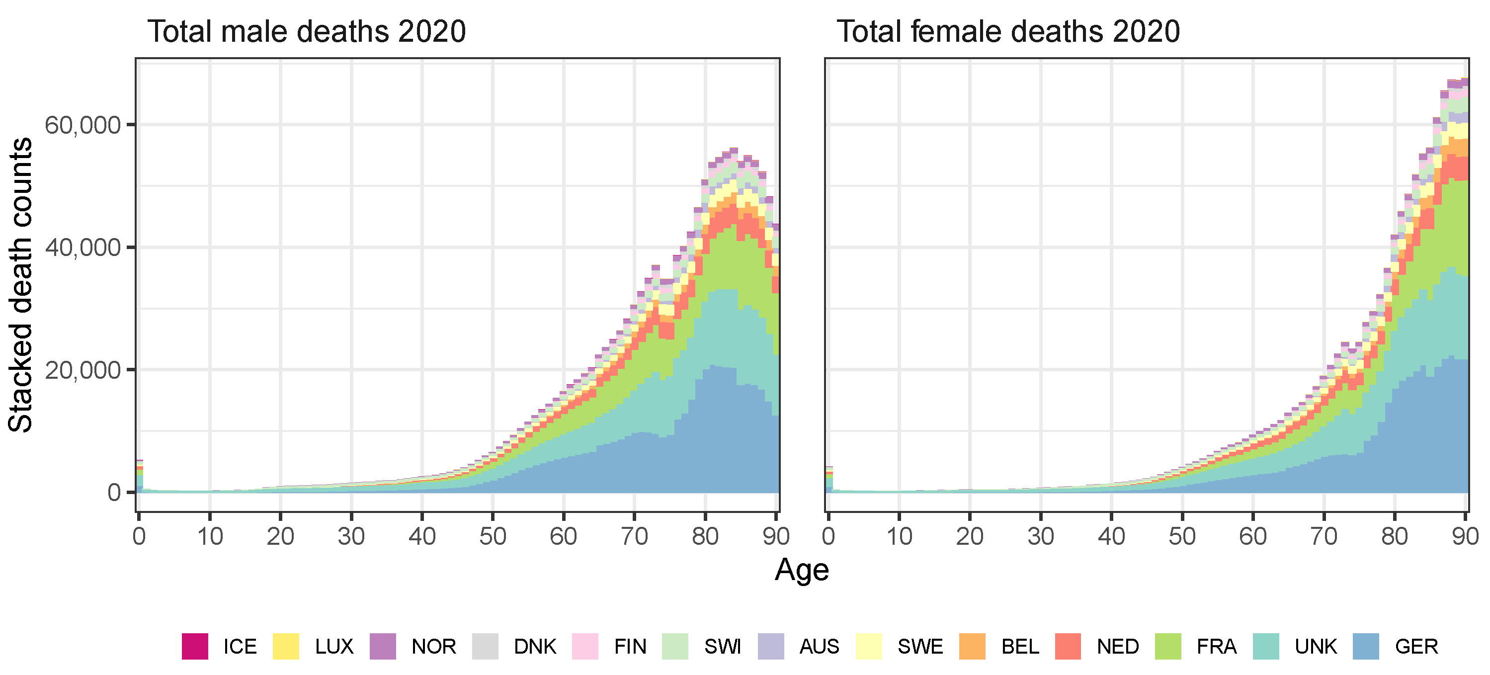
We create the annual death counts at individual ages in year t for which the statistics at individual ages have not yet been published. To do this, we take the raw death counts by age buckets reported by the STMF data series or Eurostat and allocate these to individual ages. Hereto, we extrapolate a multi-population mortality model (e.g., the IA∣BE 2020 model) to obtain mortality rate estimates in year t. Then, we combine these estimates with the (virtual) exposures from year t to obtain virtual death counts in year t. In this protocol, we make sure that the virtual death counts aggregated over an age bucket in year t correspond to the actual number of deaths in that age bucket from the STMF data series or Eurostat. Appendix C provides the technical details. Figure 4 shows the stacked European number of deaths in 2020 for males (left panel) and females (right panel). Figure 5 shows the evolution of deaths over time for Belgium, the United Kingdom and Germany. The excess of deaths in 2020 due to COVID-19 is clearly visible at old ages.
4.3. Applying the Protocol to the Multi-Population Data Set to Recalibrate the Li and Lee Mortality Model for the Belgian Population
Table A1 in Appendix A indicates for which countries and for which years the data set must be supplemented with information from the weekly deaths and exposures registered in age buckets from the STMF data series or Eurostat. For those years and those countries, we apply the protocol from Section 4.1 and Section 4.2 to move from the weekly deaths and exposures in age buckets to annual data at an individual age level. We then recalibrate the Li and Lee model for the Belgian population on an extended data set up to and including the year 2020. The United Kingdom is the only country for which we have to create virtual exposures and death counts at individual ages for both the years 2019 and 2020. Next, we only have to create virtual exposures for the year 2020 for Belgium since we retrieve the death counts in 2020 at individual ages from Statbel.18 Moreover, at the time of writing, the HMD already provides deaths and exposures for Denmark in 2020 at the level of individual ages. For all other considered European countries, we have to create virtual deaths and exposures for the year 2020. Appendix D validates the protocols. We do this by comparing the observed exposures from Denmark and the observed death counts from Denmark and Belgium in the year 2020 with the virtual deaths and exposures constructed by using the protocols in Appendix B and Appendix C.
5. Assessing the Impact of a Pandemic Shock on the Multi-Population Mortality Model
The IA∣BE 2020 mortality model (Antonio et al. 2020) is calibrated on data from 1988–2018 (European trend) and 1988–2019 (Belgium-specific trend). Using the protocol from Section 4, we are able to collect data from 1988–2020 for all 13 countries under consideration in this multi-population mortality model. As a starting point, we recalibrate the mortality model on the data set up to and including the pandemic year 2020. However, since the mortality shock takes place in the last year of our calibration period , it has a major impact on the estimated drift term in the assumed random walk with drift process for the European period effect (see Equation (4)). This, in turn, severely impacts the mortality and life expectancy forecasts, as the year 2020 is the starting year to generate future scenarios of mortality (Section 3.3).
With the roll-out of the four COVID-19 vaccines, approved by the European Medicine Agency, a more optimistic scenario is that post-pandemic mortality rates will continue their improvement at a rate that is similar to pre-pandemic levels. Section 5.1 introduces a method to put this scenario into practice. We limit the weight of the pandemic data point (the year 2020) in the four-dimensional Gaussian log-likelihood (see Equation (5)) to estimate the time series parameters in Equation (4). However, this strategy uses the pandemic 2020 observations as a starting point to generate future mortality projections. Therefore, we still observe a fairly large difference between the short-term future mortality rates and life expectancies when comparing the results obtained with the original IA∣BE 2020 model and the recalibrated mortality model.
The impact of the pandemic year 2020 concentrates on old age mortality rates, as Figure 5 illustrates. The stochastic multi-population mortality projection model of type Li and Lee (Li and Lee 2005), as specified in Equation (2), cannot capture this age-specific effect of the pandemic on the mortality rates. Indeed, first, the upward jump in the estimated common European period effect is driven by the deterioration in mortality rates for the older ages. Second, the common age effect is larger for the younger ages than for the older ages (see Figure 6 and Figure 7 later on). Since we multiply the common period effect with the common age effect in Equation (2), the mortality deterioration actually has the largest impact on the fitted mortality rates for the younger ages. Therefore, the Li and Lee model overestimates the observed mortality rates at the younger ages and underestimates the deterioration of the mortality rates at the older ages in the pandemic year 2020.
In light of the above discussion, Section 5.2 introduces a method that slightly changes the model specifications in Equation (2). We here impose that the fitted death rates in the pandemic year 2020 are equal to a weighted average of the observed death rates in the year 2020 and the pre-pandemic rates in 2019. By giving a zero weight to the observed death rates in 2020, we can investigate the situation where we completely ignore the COVID-19 pandemic and are of the belief that the post-pandemic death rates in 2021 immediately recover to pre-pandemic levels.
5.1. Limiting the Time Series Likelihood Contribution of the Pandemic Data Point
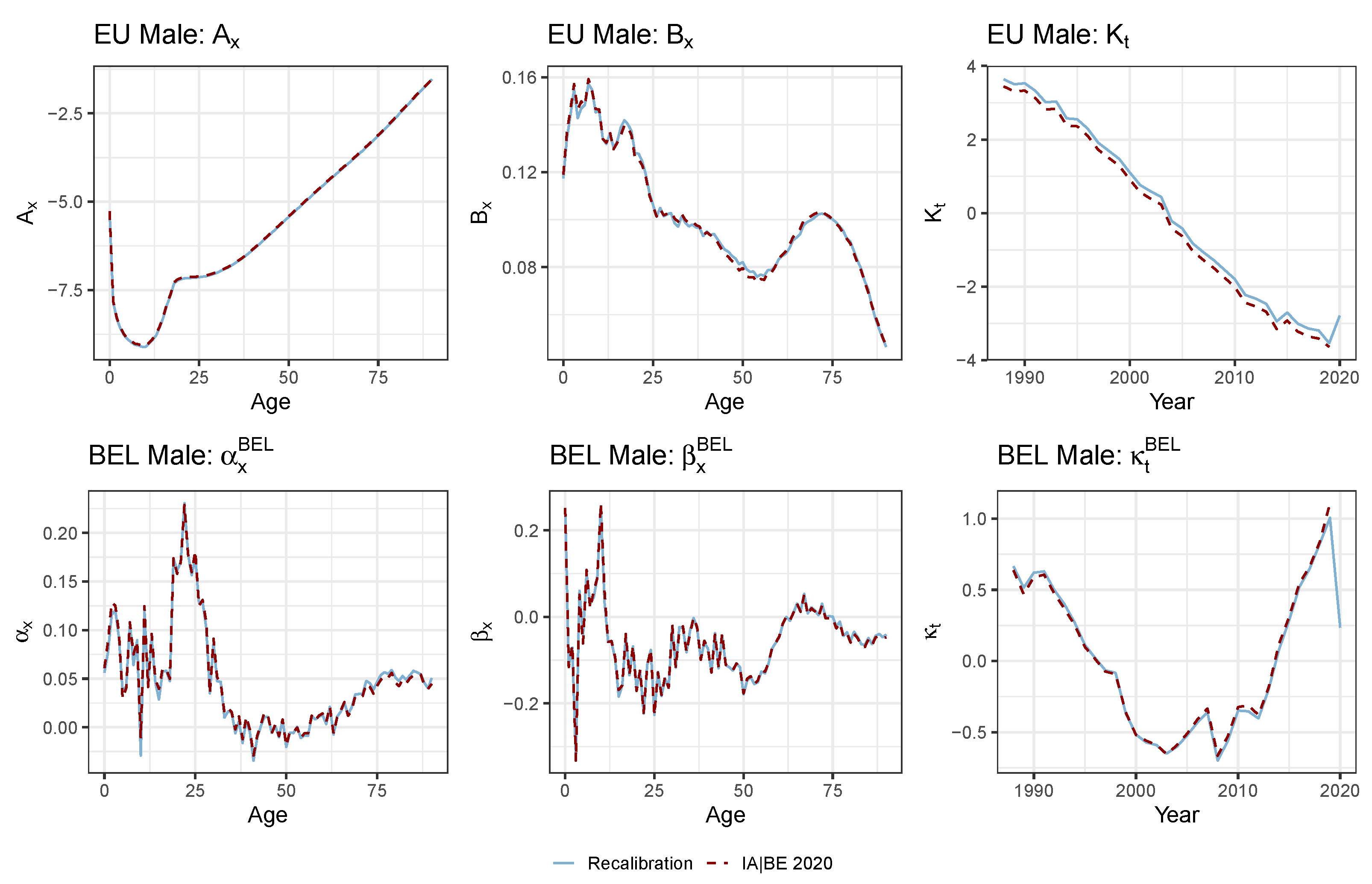
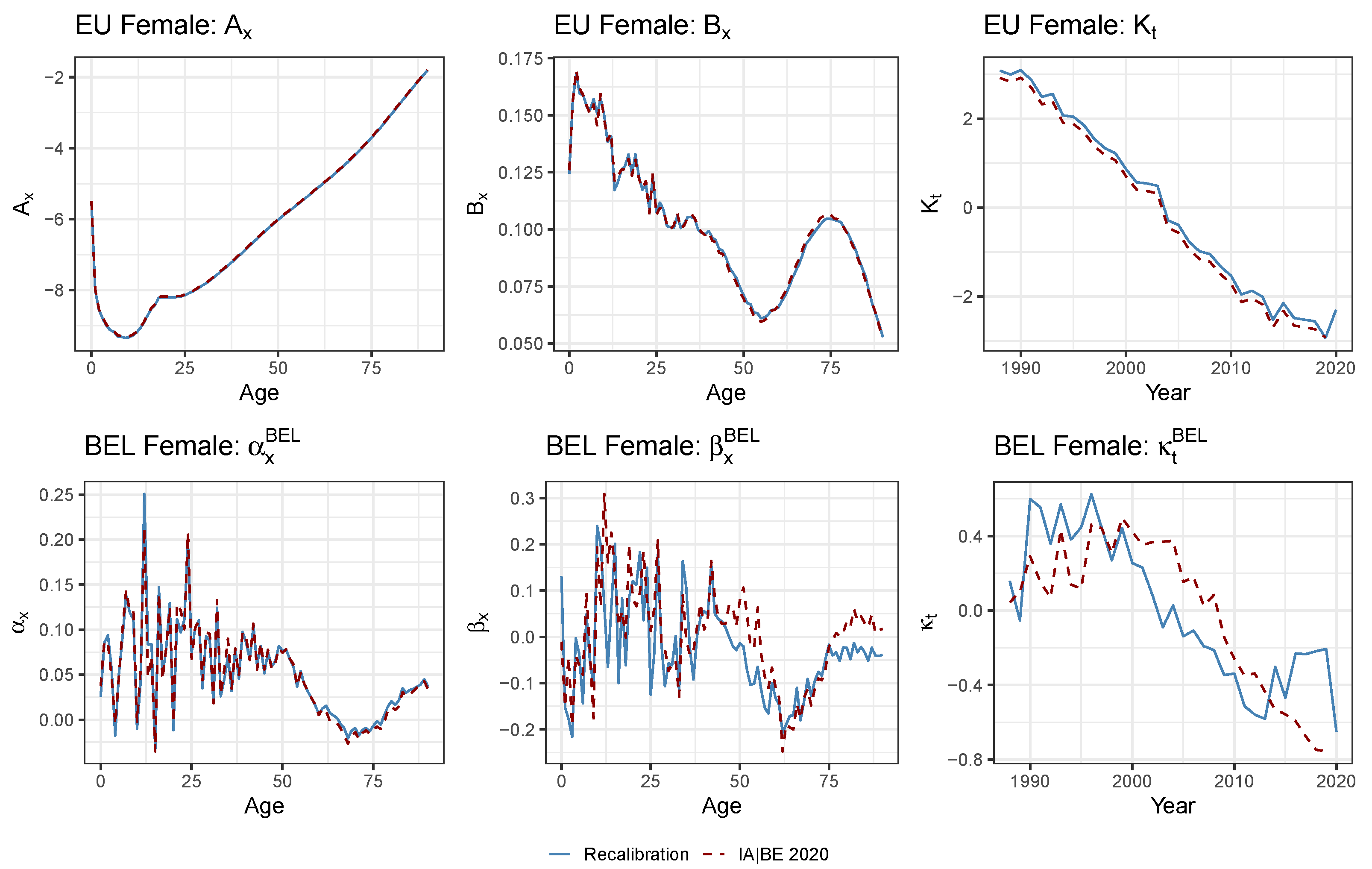
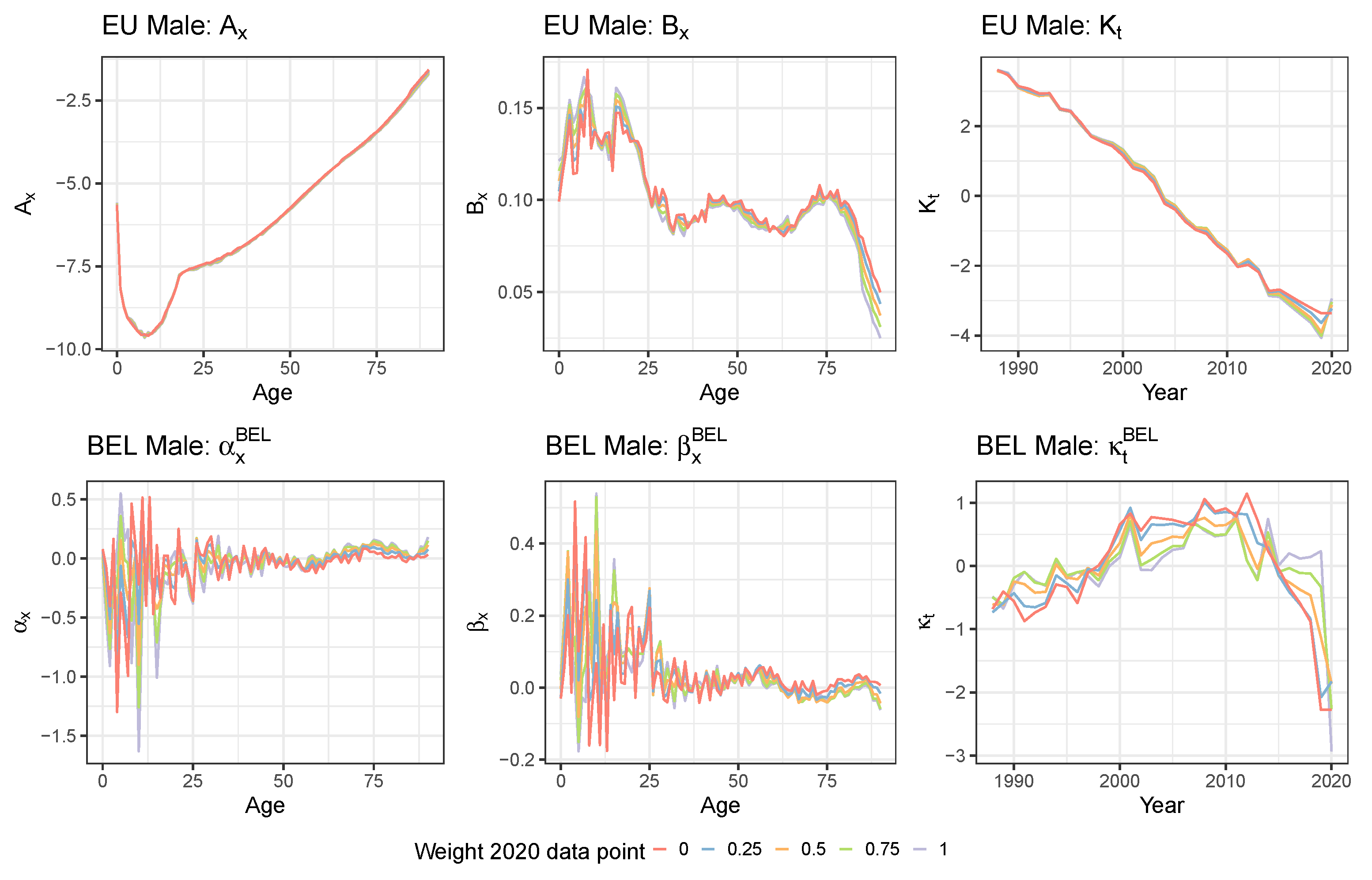
We first perform a simple recalibration of the mortality model on the data set including the (virtually created) death counts and exposure points up to the year 2020. This recalibration is completely in line with the model choices and design principles underneath IA∣BE 2020. Figure 6 and Figure 7 show the recalibrated Li and Lee parameters for males (top panels) and females (bottom panels). We visualize these together with the parameter estimates from the original IA∣BE 2020 model. We do not observe any substantial differences in the calibrated age-dependent parameters (European trend), and (Belgian deviation). The recalibrated common period effect reveals a clear upward jump in the year 2020 for both males and females to account for the increase in observed mortality rates (see Figure 1 and Figure 5). The sharp decline in the male Belgium-specific period effect in the year 2020 implies that the male Belgian mortality rates do not diverge further from the European mortality rates. In addition, we observe larger differences between the original and the recalibrated Belgium-specific period effect for females, i.e., .
We use the specification proposed in Section 3.2 for the time dynamics. However, we now limit the contribution of the pandemic data point in the four-dimensional Gaussian log-likelihood in the estimation of the four-dimensional time series for (see Equation (5) in Section 3.2). Hereto, we introduce weights in the Gaussian log-likelihood:
We specify for and consider five possible scenarios for . This is . We follow the same approach for the projection set-up as in Section 3.3. The use of a weighted log-likelihood function allows for assessing the impact of the contribution of the pandemic data point on the projections of the time-specific parameters, the mortality forecasts and the life expectancy predictions.
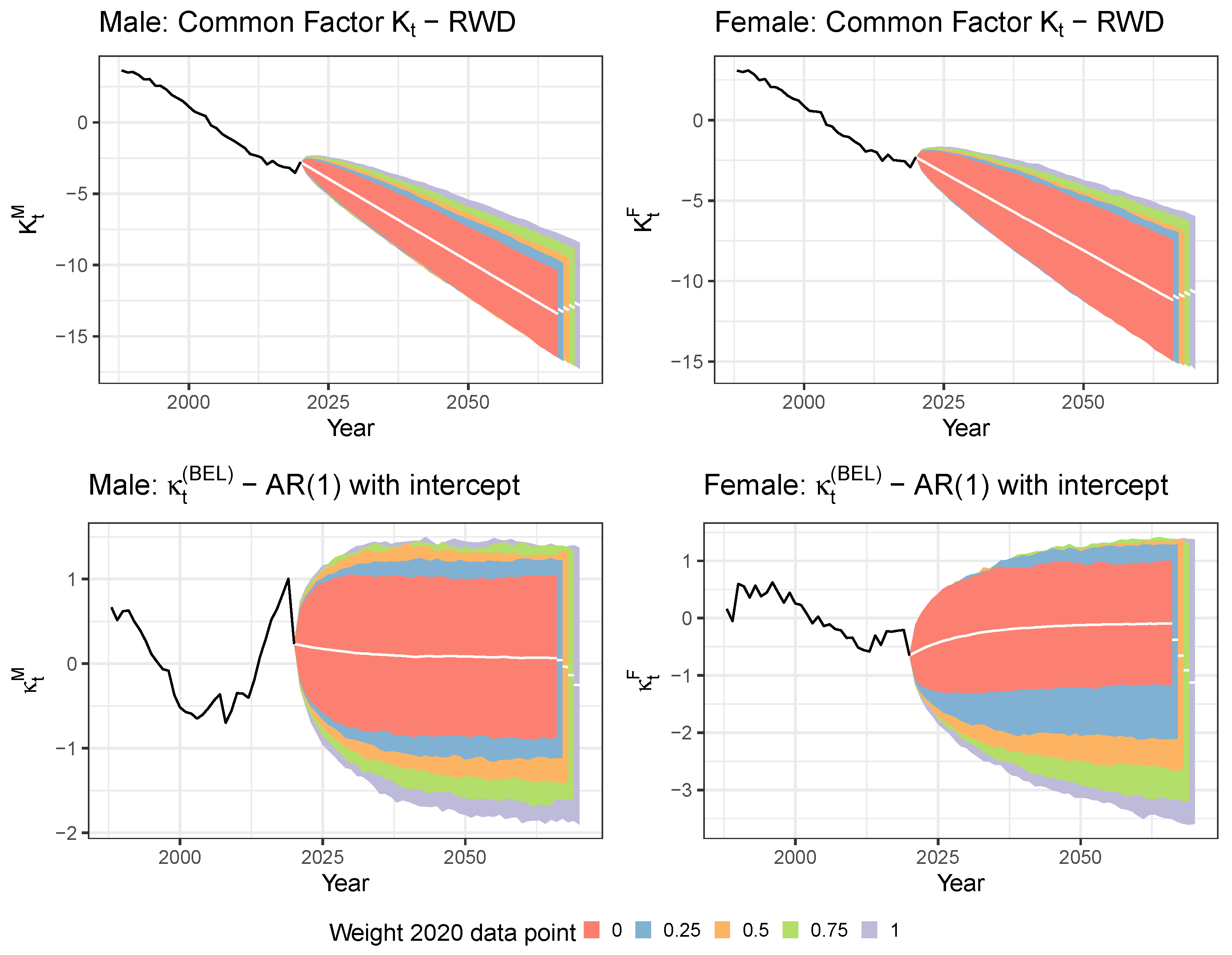
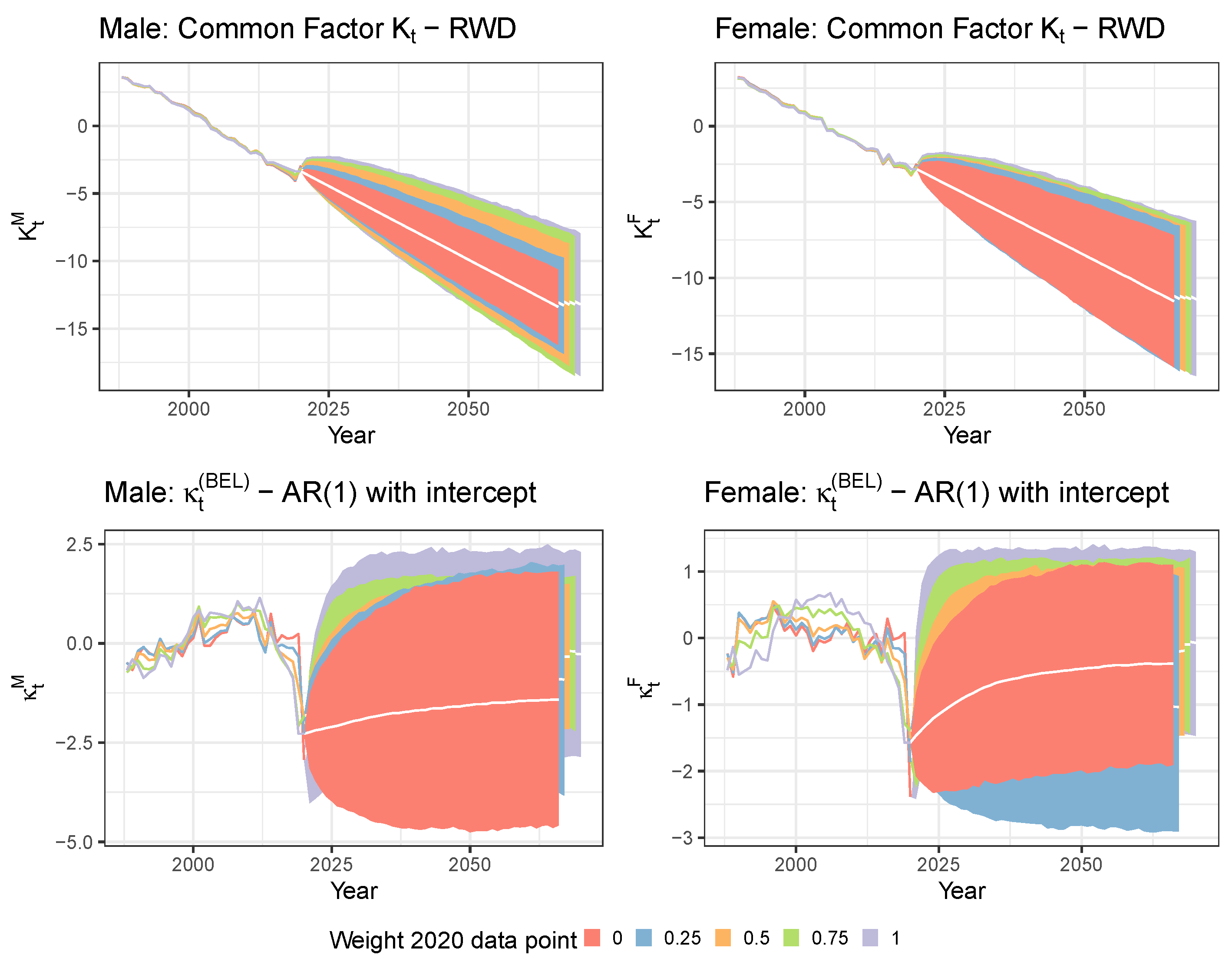
Figure 8 shows the projection of the calibrated European and Belgium-specific period effects and for males and females. First, a lower weight for the likelihood contribution of the 2020 data point leads to less variability in the simulations. Second, lowering the 2020 weight leads to a larger (absolute) value of the drift parameter in the RWD process for the common period effect . In addition, it leads to a faster long-term mean reversion for the Belgium-specific period effect . This is confirmed by Table 1 in which we show the time series parameter estimates across the five different weighting scenarios of the 2020 data point. In the table, we also report the time series parameter estimates obtained in the original IA∣BE 2020 model. The latter estimates should be broadly in line with the estimates of the zero weight scenario. However, some deviations may occur because the original IA∣BE 2020 model uses the calibration period 1988–2018 to model the European mortality trend, while our recalibration uses the calibration period 1988–2020. The AR(1) parameter estimates reveal that the Belgian deviation for females becomes less stable when the 2020 data point fully contributes to the Gaussian likelihood, i.e., the estimate is very close to one. A potential drawback of this method to deal with the pandemic data point is that the projections jump off from the impacted estimates and in the year 2020.
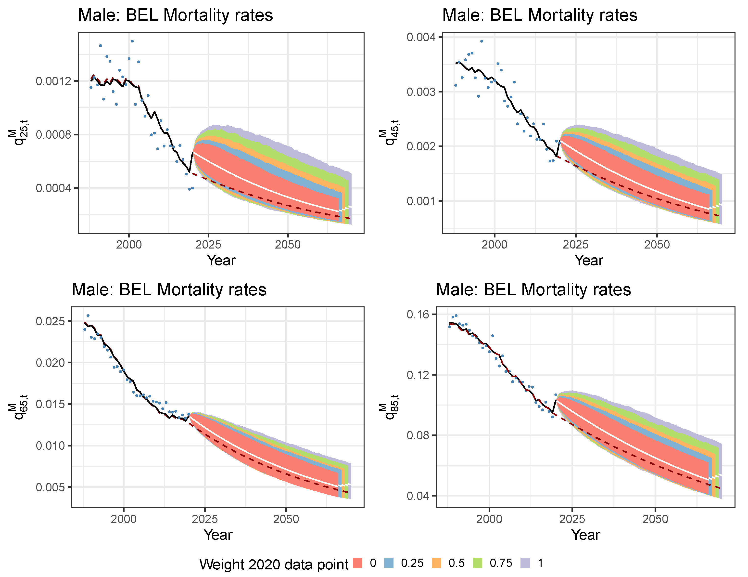
Figure 9 shows the observed, calibrated and simulated Belgian mortality rates for ages 25, 45, 65 and 85 from the recalibrated mortality model and the original (pre COVID-19) IA∣BE 2020 model. We observe a rather poor in-sample fit of the male mortality rate for age 25 in 2020 since the Li and Lee mortality model is not able to capture the observed differences in excess of mortality between the younger and older ages. Because of the estimated, in sample increase in mortality rates at all ages, the projected mortality is clearly at a higher level in the recalibrated model compared to the projected mortality in the original IA∣BE 2020 model. In addition, limiting the time series likelihood contribution of the 2020 data point leads to lower projected mortality rates on average. The results from Figure 8 confirm this.
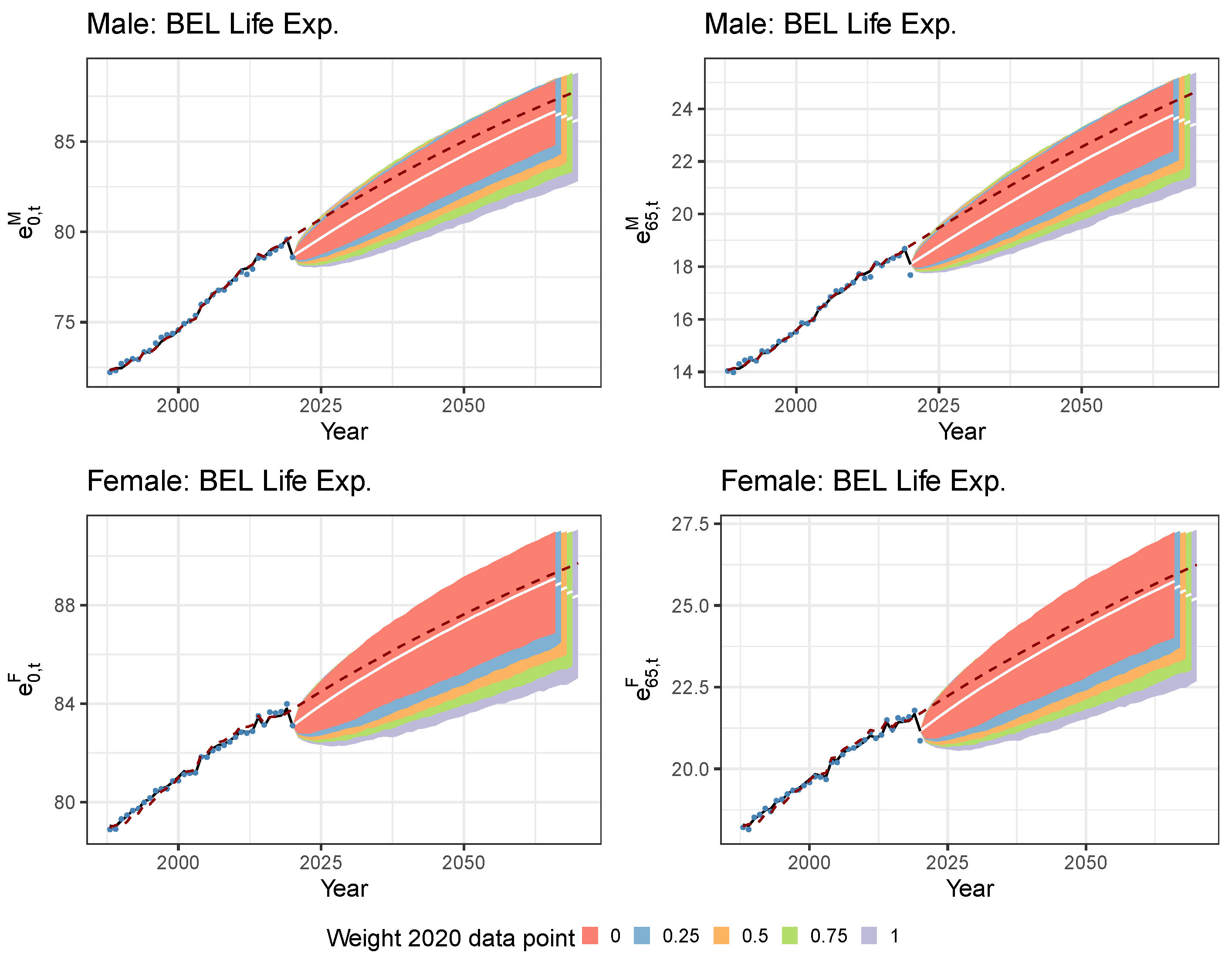
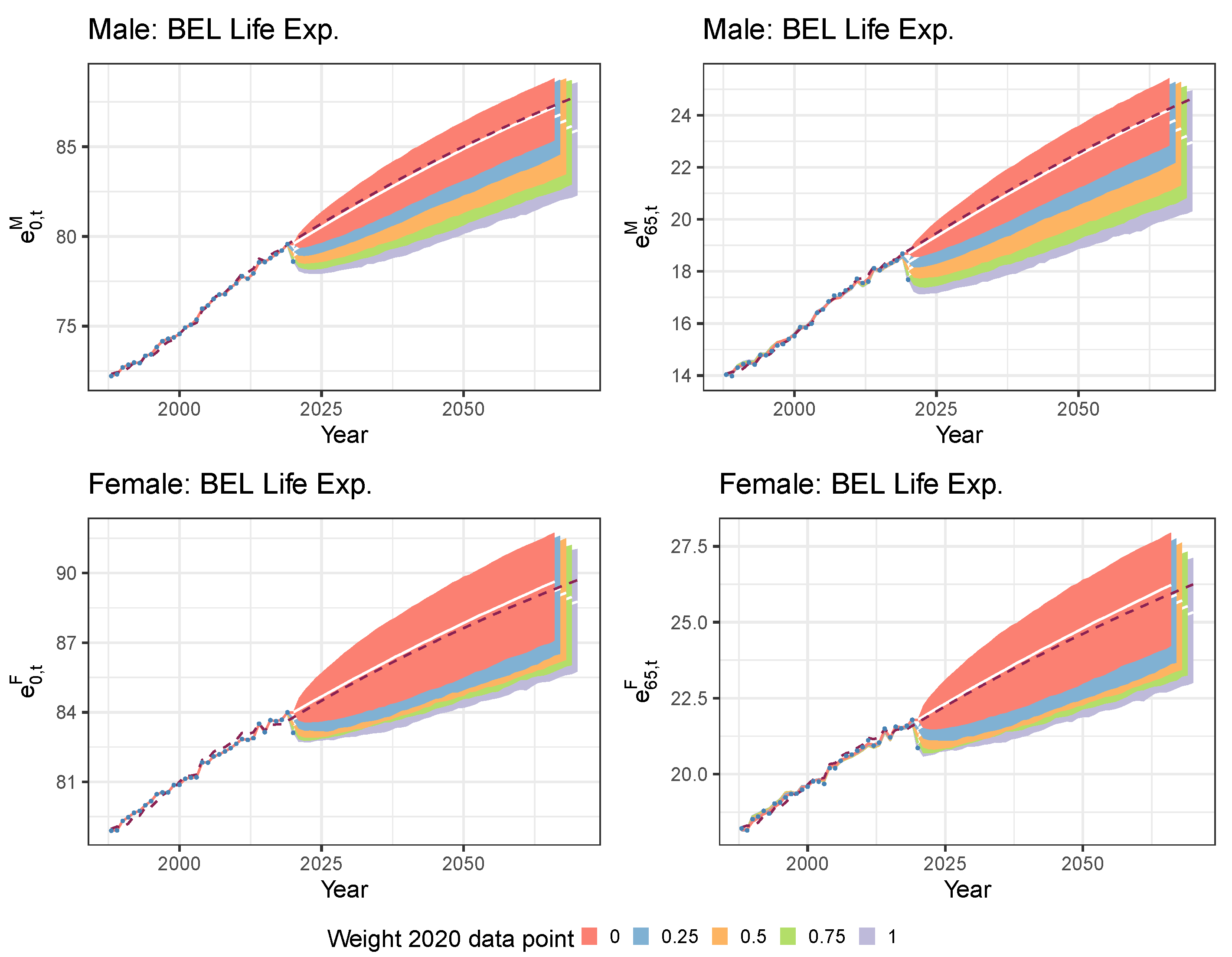
We are now ready to assess the impact of COVID-19 on the estimated and projected period and cohort life expectancies. Figure 10 depicts the projected period life expectancies of a male and female Belgian newborn (left) and a 65 year old (right) resulting from the recalibrated mortality model (fan charts) and from the original IA∣BE 2020 model in Antonio et al. (2020) (dark red, dashed line). Table 2 then shows the best-estimates and the , median and quantiles of the 10,000 simulations for the cohort life expectancy of a 0 and 65 year old in 2020 (see Section 3.3). Both period and cohort life expectancies are negatively impacted by COVID-19. Moreover, the long-term impact of COVID-19 reduces for the recalibrated mortality model that assigns a smaller weight to the 2020 data point in the calibration step of the time dynamics. However, we still observe a clear and pronounced short-term impact of COVID-19 on the period and cohort life expectancies across all the different weighting scenarios. In addition, we also observe less uncertainty in the life expectancy simulations when a smaller weight is allocated to the 2020 data point, as the more narrow fan charts in Figure 10 indicate.
A closer look at Figure 10 reveals an over-estimation of the period life expectancy in 2020 for a 65 year old. This is primarily due to the fact that the Li and Lee model tries to achieve a good in-sample fit for both the young and the old ages. As a result, the model produces higher mortality rates than observed for the young ages and lower mortality results than observed for the older ages, as confirmed by Figure 9.
5.2. Mitigating the Impact of the Pandemic Data Point with a Lee and Miller Inspired Mortality Model
The method discussed in Section 5.1 to deal with the pandemic data point has two potential drawbacks. First, we get a poor in-sample fit of the observed mortality rates and life expectancies in the pandemic year 2020. Second, even with a low to zero weight assigned to the 2020 period effects in the time series likelihood, we obtain a clear short-term impact of COVID-19 on the predicted mortality rates and life expectancies. This scenario may be considered unrealistic in light of the effectiveness of the approved vaccines. In view of the aforementioned shortcomings, we therefore propose two modifications to the Li and Lee mortality model.
Modification 1.
A first modification consists of slightly changing the model specifications of the Li and Lee model (see Equation (2)). Hereto, note that the (central) death rate equals . Under the piecewise constant force of mortality assumption, introduced in Section 2, the maximum likelihood estimate of the force of mortality, , equals the observed death rate . Lee and Miller (2001) adjust the Lee and Carter model specification in such a way that the fitted forces of mortality in the last year of the calibration period are equal to the observed death rates in that year. This provides a solution for the poor in-sample fit at young ages in the pandemic year 2020. We extend this idea to the Li and Lee mortality model. We hereby reduce the degrees of freedom in the mortality model of Equation (2) by fixing the parameter values for and such that the fitted and observed country-specific death rates in the year 2020 match.
Modification 2.
Second, we mitigate the (short-term) impact of the pandemic data point on the mortality projections. We do this by relaxing the fact that the observed death rates are exactly the same as the fitted forces of mortality in the pandemic year 2020. Instead, we opt for a weighted average between the observed death rates in the last two years of the calibration period.
The adjusted Lee and Miller model specifications.
The two discussed modifications result in the following model specifications:19
with and . Furthermore, for , is the observed common central death rate and the observed country-specific `central death rate’ with adjusted exposure :
In addition, is the weight we assign to the observed central death rates in 2020. With the definitions in Equation (10), the case corresponds to the situation in which the observed country-specific death rates are equal to the fitted country-specific forces of mortality in the year 2020. As a consequence, the fitted and observed country-specific mortality rates also coincide in the year 2020. For this weighting scenario, we therefore get a perfect fit of the observed period life expectancy in the year 2020. Taking corresponds to the situation where the fitted mortality rates in 2020 equal the observed mortality rates in 2019. In the latter scenario, we completely ignore COVID-19 and assume that the mortality rates have not been changed over the years 2019–2020. We refer to the model, specified in Equation (9), as the adjusted Lee and Miller mortality model.
Figure 11 and Figure 12 display the calibrated parameters for males and females in the adjusted Lee and Miller mortality model. In contrast to Section 5.1, we now obtain different calibrated results for each weighting scenario. Note that the parameters and are not calibrated in this approach, but they represent the fixed values, given in Equation (9). In addition, the larger the weight , the more pronounced the upward jump in the calibrated common period effects and the larger the downward jump in the Belgium-specific period effects in the year 2020.
We use the same time dynamics and follow the same projection and simulation strategy as outlined in Section 3.2 and Section 3.3. We do not include weights in the time series likelihood (see Equation (8)) to estimate the time series parameters. Figure 13 shows the calibrated and simulated period effects in the adjusted Lee and Miller mortality model. Table 3 lists the estimated time series parameters.
Figure 14 displays the calibrated and projected mortality rates for a 25, 45, 65 and 85 year old Belgian male. A lower weight implies that the fitted mortality rates in 2020 are closer to the observed mortality rates in 2019 than those of 2020. This in turn results in an overall, better in-sample fit of the mortality rates at old ages, see e.g., the bottom right panel in Figure 14. Moreover, lowering the weight leads to results closer to the original IA∣BE 2020 model (dark red, dashed line) on average. Another noteworthy fact is the increase in the projected mortality rates for a 25 year old male (top, left panel) right after the pandemic year 2020 in the case of a larger weight . This increase is partly due the fast mean reversion of the time series (see Figure 13) in combination with larger calibrated values at the younger ages (see Figure 11 and Figure 12 for the graphs of ). Therefore, the term can become larger than the term in Equation (9) at early years in the projection period.
Figure 15 shows the estimated and projected period life expectancies for a 0 and 65 year old Belgian male (top) and female (bottom). Assigning the value zero to the weight leads to comparable results with the original IA∣BE 2020 model (dark red, dashed line). This is in line with our expectations since we actually omit the pandemic data point in the calibration step when . Table 4 depicts the cohort life expectancy in 2020 for a 0 and 65 year old male and female.
6. Addressing a Mortality Shock in a Mortality Prediction Model: A Literature Review
The adjustments and sensitivity analyses proposed in Section 5 provide a framework to assess the impact of the COVID-19 pandemic data point on a stochastic multi-population mortality projection model of type Li and Lee. Professional actuarial organisations, such as the Institute of Actuaries in Belgium and the Royal Dutch Actuarial Association, publish regular updates (e.g., every two years) of their model. In their updates, these organisations care for reproducibility, continuity and explainability of the mortality projection model. Therefore, we explicitly aim for proposed adjustments that are much in line with the original design principles of the mortality model. These ambitions are now challenged by the presence of a mortality shock. Next, to the strategies outlined in this paper, other techniques have been proposed in the literature to handle such mortality or pandemic shocks in the Lee and Carter projection model (Lee and Carter 1992).
The Lee & Carter model.
The Lee and Carter mortality model specifies the logarithm of the force of mortality as:
To forecast mortality rates, a random walk with drift model is typically assumed for the calibrated :
with the drift term and a random noise term. A standard assumption is that follows a normal distribution with mean 0 and unknown variance .
Outlier detection.
A first stream of literature puts focus on outlier detection methods. One technique is described in Lee and Carter (1992), where an intervention model is proposed to deal with the influenza epidemic in 1918 when estimating the random walk with drift model for (see Equation (12)):
with being a dummy variable equal to one in the year of the influenza epidemic. Parameter captures the size of the increase in in 1918. The dummy variable is an important component in the random walk with drift model, as the width of the prediction interval for increases significantly when Lee and Carter (1992) exclude this dummy. Li and Chan (2005) conduct a more thorough investigation of outlier detection in the period effect of the Lee and Carter model. They define a general time series outlier model for as:
where follows an outlier-free ARIMA() model. Furthermore, is the year in which outlier i occurs, the magnitude of outlier i and m the number of outliers. The term is an exogenous intervention effect whose functional form depends on the specific type of outlier i. To identify and to construct the model in Equation (13), Li and Chan (2005) apply an iterative procedure to detect outliers in the estimated residuals from the fitted ARIMA() time series model for . The discussed outlier detection methods regard mortality shocks as non-repetitive, exogenous events and try to unravel the real underlying mortality dynamics.
Jump processes.
A second stream of literature focuses on mortality modelling with jump processes. Cox et al. (2006) and Chen and Cox (2009) extend the Lee and Carter model with permanent and transitory jump effects, respectively. Let denote a random variable that indicates whether there is a jump event in year t. The probability of occurrence of a jump event is assumed to be time-independent and equal to p. For the model with permanent jump effects (Cox et al. 2006), the random walk with drift model for extends to:
where models the size of the jump in year t (if any). The ’s are assumed to be independent and identically distributed with mean m and standard deviation . Chen and Cox (2009) notice that when a jump event occurs in year t, all future (), resulting from the estimated time series model in Equation (14), will be affected. Catastrophic or pandemic shocks, such as the influenza epidemic in 1918, only have a transitory effect on the mortality rates instead of a permanent effect. Therefore, Chen and Cox (2009) extend the random walk with drift model with a transitory jump effect:
Thus, a jump event in year in this model is transitory because the jump is cancelled in year t (see in ). Furthermore, the model allows for future jump events when simulating future paths for . Zhang et al. (2021) discuss an alternative technique. As a baseline, they first model the force of mortality without COVID-19 using a Lee and Carter model. Next, they capture the pandemic shock of COVID-19 by multiplying the baseline force of mortality with a temporary mortality jump process where jump events arrive at a certain determined pandemic arrival rate .
These jump processes do not allow for an age-specific effect of the jump event, e.g., a pandemic shock, on the mortality rates. Therefore, Liu and Li (2015) add a transitory jump component to the model specification in Equation (11):
with a time and age-dependent jump effect and a dummy variable which equals one if a jump event occurs in year t. This appears to be a useful addition to the Lee and Carter model to capture the age-specific effect of COVID-19 on the observed mortality rates in 2020 (see Figure 5).
Extreme value theory.
Recent literature also investigates the use of extreme value theory to accurately forecast mortality rates during periods of extreme events. Gungah and Narsoo (2021) propose the EVT modified Lee and Carter model. Hereto they start from the usual random walk with drift model for the period effect in Equation (12). Gungah and Narsoo (2021) now assume that the ’s, defined as , are independent and follow an extreme value distribution instead of the normal distribution. In particular, the ’s are assumed to be realizations from a two-parameter Generalized Pareto Distribution with shape parameter and scale parameter . The use of EVT in the random walk with drift model for allows for modelling sudden mortality jumps. Similar work is done in Chen and Cummins (2010), with an application in longevity risk securitization.
7. Conclusions and Outlook
This paper examines different methods to deal with a pandemic data point in the calibration and projection set-up of a stochastic multi-population mortality projection model, in casu the Li and Lee model. When this data point corresponds to the last observed year in the calibration period, it severely affects the drift parameter estimation in the random walk with drift process to model the common European period effect for males and females. To control this impact, we propose to make changes in either the projection strategy (Section 5.1) or in the model specifications (Section 5.2) itself. We do this by restricting the impact of the pandemic year through the inclusion of weights in the calibration or projection step.
There are still many uncertainties about the future evolution of COVID-19. COVID-19 may have impacted mortality rates during just one or two years, or future years may be affected as well. Future relevant work may focus on more thorough modifications of the Li and Lee model so that it can automatically absorb pandemic shocks rather than assigning a subjective weight to this pandemic data point. Section 6 provides a literature review that discusses techniques to handle extreme mortality events in a Lee and Carter mortality projection model. Examples include outlier detection methods, permanent and transitory jump processes, and the use of extreme value theory.
In addition, several assumptions underneath the stochastic multi-population mortality projection model of type Li and Lee may require further investigation. Future work may put a focus on including a cohort effect in the model. This can be useful when COVID-19 has a long-lasting effect on the health of people who have been severely affected by COVID-19, e.g., hospitalized persons. Extending the techniques outlined in Section 6 to a mortality model of type Li and Lee is another direction of future work. Next, to this, one can further examine the selection of the weight , assigned to the observed death rates in 2020 in Section 5.2, in a data-driven way. One idea is to include as a parameter that can be optimally chosen in the calibration set-up. Finally, future research may also focus on the performance of Kannisto’s method to extrapolate the mortality rates above the age of 90 in the presence of a pandemic shock.
Author Contributions
Conceptualization, J.R., K.A. and S.D.; methodology, J.R., K.A. and S.D.; software, J.R.; validation, K.A.; formal analysis, J.R. and K.A.; investigation, J.R. and K.A.; resources, J.R. and K.A.; data curation, J.R.; writing—original draft preparation, J.R.; writing—review and editing, K.A. and S.D.; visualization, J.R. and K.A.; supervision, K.A. All authors have read and agreed to the published version of the manuscript.
Funding
This research received no external funding.
Institutional Review Board Statement
Not applicable.
Informed Consent Statement
Not applicable.
Data Availability Statement
The annual mortality data at an individual age level is publicly available on the Human Mortality Database (https://www.mortality.org/, accessed on 13 April 2021), Eurostat (https://ec.europa.eu/eurostat, accessed on 13 April 2021) and Statbel (https://statbel.fgov.be/en, accessed on 13 April 2021). The weekly mortality data collected in age buckets is publicly available on Eurostat (accessed on 30 July 2021) and from the Short-Term Mortality Fluctuations Data series on the Human Mortality Database (accessed on 30 July 2021).
Acknowledgments
Katrien Antonio acknowledges the support of the research chair DIALog, sponsored by CNP Assurances, and the support of the Research Centre for Longevity Risk at the University of Amsterdam.
Conflicts of Interest
The authors declare no conflict of interest. Sander Devriendt is employed by the National Bank of Belgium in addition to his research mandate at KU Leuven. However, this paper reflects only his personal views as a researcher and not the views of his employer.
Appendix A. Data Sources

Table A1.
Overview of the data sources used for each country in the stochastic multi-population mortality projection model of type Li and Lee. The data sources ‘HMD’, ‘EURO’ and ‘STATBEL’ refer to the Human Mortality Database, Eurostat and the Belgian statistical institute Statbel, respectively. They provide mortality data on an annual basis and at the level of individual ages. ‘HMD’ is our primary data source. We use the other two data sources to supplement the annual deaths and exposures at the individual age level for the more recent years 2018–2020 where possible. Because these data sources are subject to a significant reporting delay of sometimes several years (e.g., for the United Kingdom), we consult the Short-Term Mortality Fluctuations (STMF) Data series and the weekly death statistics available at Eurostat (EURO.W) to supplement our dataset until the year 2020. The latter two data sources provide weekly mortality statistics registered in age buckets. We convert these to annual mortality statistics at the individual age level using the protocol in Section 4.
| Country | Exposures | Deaths | ||||||
|---|---|---|---|---|---|---|---|---|
| 2017 | 2018 | 2019 | 2020 | 2017 | 2018 | 2019 | 2020 | |
| AUS | HMD | HMD | HMD | STMF | HMD | HMD | HMD | EURO.W |
| BEL | HMD | HMD | EURO | STMF | HMD | HMD | EURO | STATBEL |
| DNK | HMD | HMD | HMD | HMD | HMD | HMD | HMD | HMD |
| FIN | HMD | HMD | HMD | STMF | HMD | HMD | HMD | EURO.W |
| FRA | HMD | HMD | EURO | STMF | HMD | HMD | EURO | STMF |
| GER | HMD | EURO | EURO | STMF | HMD | EURO | EURO | STMF |
| ICE | HMD | HMD | EURO | STMF | HMD | HMD | EURO | EURO.W |
| LUX | HMD | HMD | HMD | STMF | HMD | HMD | HMD | EURO.W |
| NED | HMD | HMD | HMD | STMF | HMD | HMD | HMD | EURO.W |
| NOR | HMD | HMD | EURO | STMF | HMD | HMD | EURO | EURO.W |
| SWE | HMD | HMD | HMD | STMF | HMD | HMD | HMD | EURO.W |
| SWI | HMD | HMD | EURO | STMF | HMD | HMD | EURO | EURO.W |
| UNK | HMD | HMD | STMF | STMF | HMD | HMD | STMF | STMF |
Appendix B. Constructing Virtual Exposure Points
We create virtual annual exposures for individual ages 0–90, years 2019–2020 and for each country that is included in the calibration of the common, multi-population trend in the Li and Lee mortality projection model (Section 3.4).20 We explain our strategy to create virtual exposures for Belgium in the year 2020, but we follow a similar approach for any other country that is part of this common mortality trend.
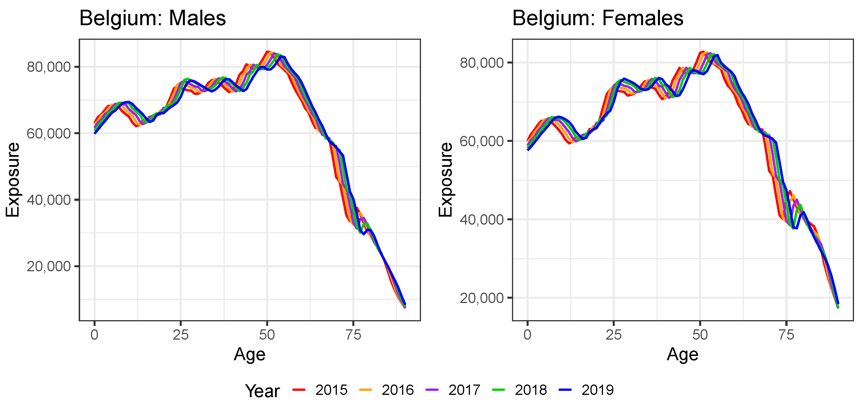
Figure A1 shows the observed exposures in Belgium as a function of age over the years 2015–2019. These exposures are retrieved from HMD and Eurostat (see Table A1). The exposure function has a similar pattern shifted to the right with one age in each subsequent year t. This is in line with our intuition since people aged x in year t become part of the group at risk aged in year , in case of survival. A rough approximation of the exposure at age in year , i.e., is thus the exposure at age x in year t minus the number of deaths at age x in year t, i.e., .
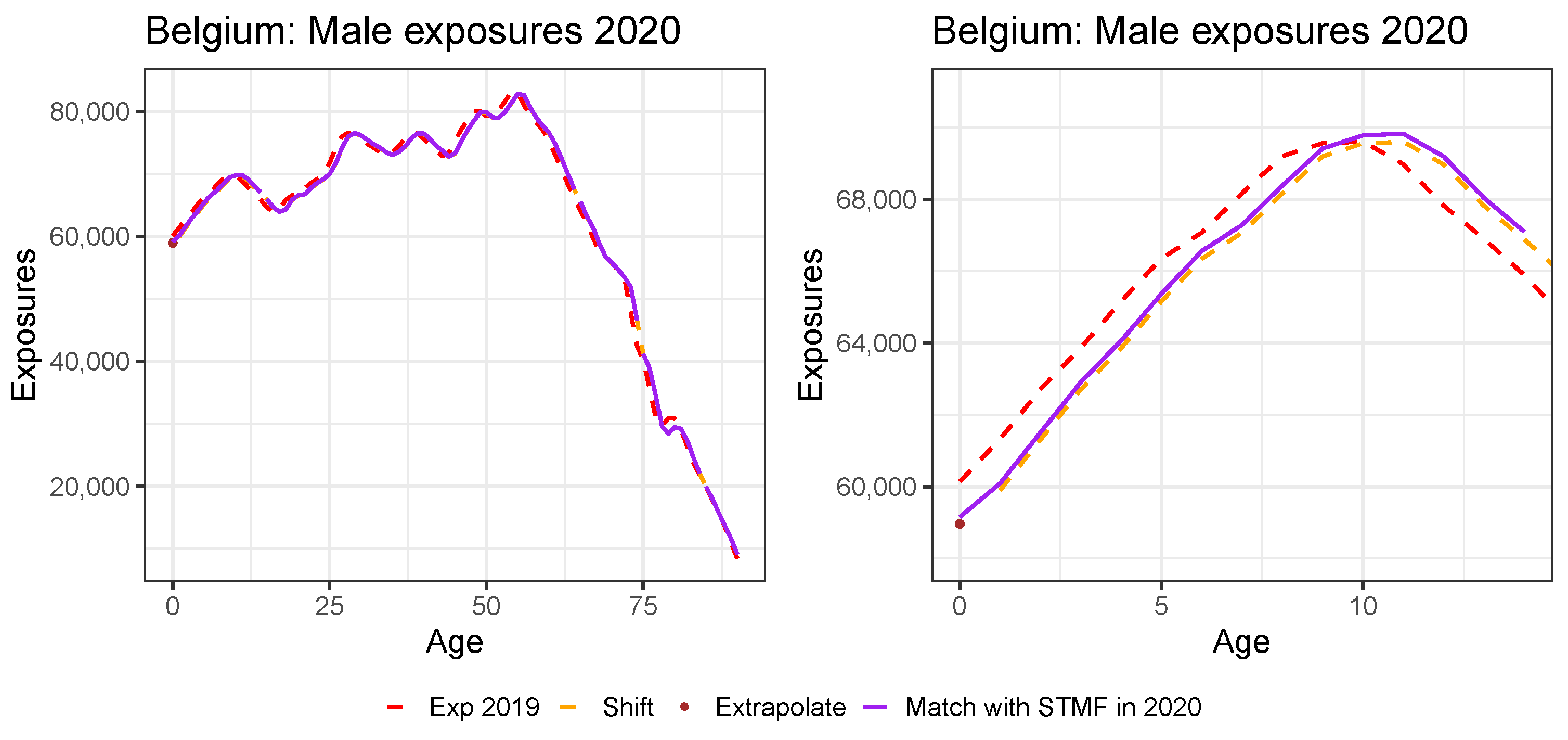
We use the above reasoning to create virtual annual exposures for 2020. Figure A2 graphically explains the strategy for Belgian males. First, we start from the observed annual exposures in the most recent available year (in casu 2019 for Belgium, using Eurostat) and visualize these as a function of age (red, dashed line). Second, we shift this 2019 exposure curve one age to the right and subtract the number of deaths at age x in year t, i.e., we define for . This results in the orange, dashed line. This newly created curve is undefined at the age of zero because of the shift to the right. Therefore, in a third step, we linearly extrapolate the orange, dashed line to zero.21 This choice is justified by the linear pattern of the exposure function at young ages. We obtain the brown exposure point in Figure A2.
Figure A1.
The exposures of Belgium for ages 0–90 and years 2015–2019. Data from HMD until the year 2018 and from Eurostat for the year 2019.
Figure A1.
The exposures of Belgium for ages 0–90 and years 2015–2019. Data from HMD until the year 2018 and from Eurostat for the year 2019.

Figure A2.
The virtual exposure for Belgium in the year 2020, for males. At the right, we show a snapshot for the age range 0–14.
Figure A2.
The virtual exposure for Belgium in the year 2020, for males. At the right, we show a snapshot for the age range 0–14.

In a last step, we match the new exposure function of 2020, i.e., , with the exposures collected in age buckets from the STMF data series, as shown in Table A2. Hereto, we consider an age bucket and define the virtual annual exposures as:
for (for example) and . Intuitively, we vertically scale a section of the orange dashed line, corresponding to a certain age bucket, such that the summed exposure within this age bucket corresponds to the total exposure in the same age bucket of Table A2. The right panel of Figure A2 shows this strategy for the age bucket , where the purple line shows the final virtual exposures at individual ages for Belgium in the year 2020.
Table A2.
The male and female Belgian exposures in 2020 in age buckets, obtained from STMF.
| Age Bucket | Male Exp. | Female Exp. |
|---|---|---|
| 988,713.02 | 944,379.40 | |
| 3,699,434.72 | 3,638,808.41 | |
| 568,101.96 | 618,244.99 | |
| 305,175.72 | 399,015.96 | |
| 112,577.56 | 223,565.55 |
We apply a slightly different strategy for the exposure reported for ages in the open age bucket on the STMF data series. The underlying idea is that we want to distribute the extra exposure (from the STMF data series) minus (from HMD) evenly across the ages , i.e., ages (the assumed maximum age). Hereto, we calculate the shift , as follows:
We then apply this shift to go from to :
for ages .
We repeat this procedure for all 13 European countries. In case there is no exposure data available for 2019 on the HMD (see Table A1 in Appendix A), we start from the exposure curve for 2019 reported on the HMD or Eurostat and repeat the procedure two times to generate data points for the years 2019–2020.
Appendix C. Constructing Virtual Death Counts
We construct virtual annual death counts at individual ages 0–90, years 2019–2020 and for each country that is included in the calibration of the common, multi-population trend in the Li and Lee mortality projection model (Section 3.4).22 In explaining our strategy, we focus on constructing virtual 2020 death counts at an individual age level for the Netherlands, but a similar approach can be taken for any other country that is part of this common mortality trend.
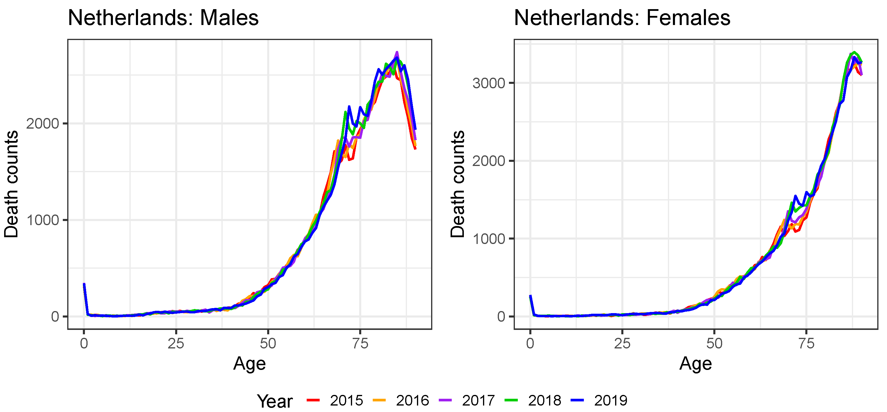
Figure A3 shows the observed annual deaths in the Netherlands across ages 0–90 and over the years 2015–2019 for males (left) and females (right). In line with our discussion about the pattern of the exposure curve in Figure A1, we observe a time-effect in these death counts, e.g., the bumps in the deaths pattern move to the right each consecutive year. We keep this in mind to construct virtual deaths for the year 2020.
We propose the following strategy. Using a Li and Lee mortality model that is calibrated only on the observed annual deaths and exposures from HMD and/or Eurostat, we project the fitted force of mortality over the next year(s) (see Section 3.3). Similar to the discussion in Antonio et al. (2020), we choose the starting year of the calibration period in the Li and Lee mortality model such that we retrieve stable AR(1) processes for both the male and female Dutch period effect. This motivates the use of starting year 1970 for the case of the Netherlands. Under the assumption of a piecewise constant force of mortality, the maximum likelihood estimate of the force of mortality then equals
with c the country of interest, i.e., the Netherlands in the example under consideration.
Figure A3.
The death counts of the Netherlands for ages 0–90 and years 2015–2019. Data from HMD.

Note that we create virtual annual exposures for the Netherlands in the year 2020 according to the strategy explained in Appendix B. Using Equation (A2), we can then easily make the transition to virtual death counts . In a next step, we match these expected deaths with the information we retrieve from the weekly deaths data on Eurostat or the STMF data series. For the Netherlands, we work with the weekly death counts in age buckets of length 5 from Eurostat, see Table A3.
Table A3.
The male and female Belgian death counts in 2020 in age buckets, obtained from Eurostat.
| Age Bucket | Male Deaths | Female Deaths |
|---|---|---|
| 410 | 325 | |
| 27 | 27 | |
| 41 | 38 | |
| 115 | 68 | |
| ⋯ | ⋯ | ⋯ |
| 12,730 | 9202 | |
| 15,125 | 12,899 | |
| 14,737 | 17,246 | |
| 12,231 | 24,974 |
Having extracted the weekly deaths on Eurostat, we now return to the construction of the virtual deaths in 2020 at individual ages 0–90. Figure A4 graphically explains this construction for Dutch males. The red line shows the observed number of male deaths in the Netherlands for the year 2019 from the HMD. Applying the Li and Lee mortality forecasting strategy of Section 3.3 to the Netherlands, we first project the force of mortality for the year and then calculate the estimated expected number of deaths . This corresponds to the orange line in Figure A4. Similar to the exposure matching principle in Appendix B, we then match the orange death curve of 2020 with the death counts collected in age buckets in 2020 from Eurostat, as given in Table A3.
Denote for the fitted death counts at age x and time t as obtained from the orange line in Figure A4. We consider an age bucket and define the virtual annual death counts as:
for and . Intuitively, we again vertically scale a section of the orange line, corresponding to a certain age bucket, such that the combined number of deaths within this age bucket corresponds to the total number of observed deaths in the same age bucket from Eurostat. This matching principle results in the purple line in Figure A4. The right panel of Figure A4 illustrates the results for the age bucket . This procedure leads to annual death counts , now evaluated at individual ages.
Figure A4.
Construction of the virtual deaths in individual ages in the Netherlands for 2020.

The last age bucket is an open age bucket. This implies that we have to modify our strategy outlined in Equation (A3) to define the virtual death count at age 90 in 2020:
and is a gender-specific rate, which we assume to be country-independent. For example, means that of the deaths, at ages 90 or higher, occur at age 90. Based on the observed ratios of Belgium and Denmark in 2020,23 we select and for males and females, respectively.
We repeat this procedure for every European country in the study with the following country-specific data adjustments. For the United Kingdom, we do not have the deaths at time yet. In this case, we construct a Li and Lee mortality model for the country of interest with a shorter calibration period, ending with the year 2018. In addition, each country has its own starting year of the calibration period for stability reasons, e.g., the year 1970 for the Netherlands. We can then construct death counts for the year 2019 and 2020 (for each scenario) by projecting the force of mortality for the years 2019–2020 and by performing the matching principle at both years.
Moreover, for three of the European countries, namely Germany, France and the United Kingdom, we work with the weekly death counts in age buckets from the STMF data series, rather than from Eurostat.24 For these countries, we apply the strategy outlined above, although we use larger age buckets.
Appendix D. Validation of the Constructed Virtual Death Counts and Exposure Points
Appendix B and Appendix C propose a protocol to extend the multi-population mortality dataset with virtual exposures and death counts at individual ages 0–90 in the years 2019–2020. Table A1 in Appendix A reveals that we already have data available at the level of individual ages in the year 2020 for Denmark (exposures and deaths ) and Belgium (deaths ). We validate the protocols by comparing these observed deaths and exposures in the year 2020 with the virtually created deaths and exposures obtained by the approaches in Appendix B and Appendix C.
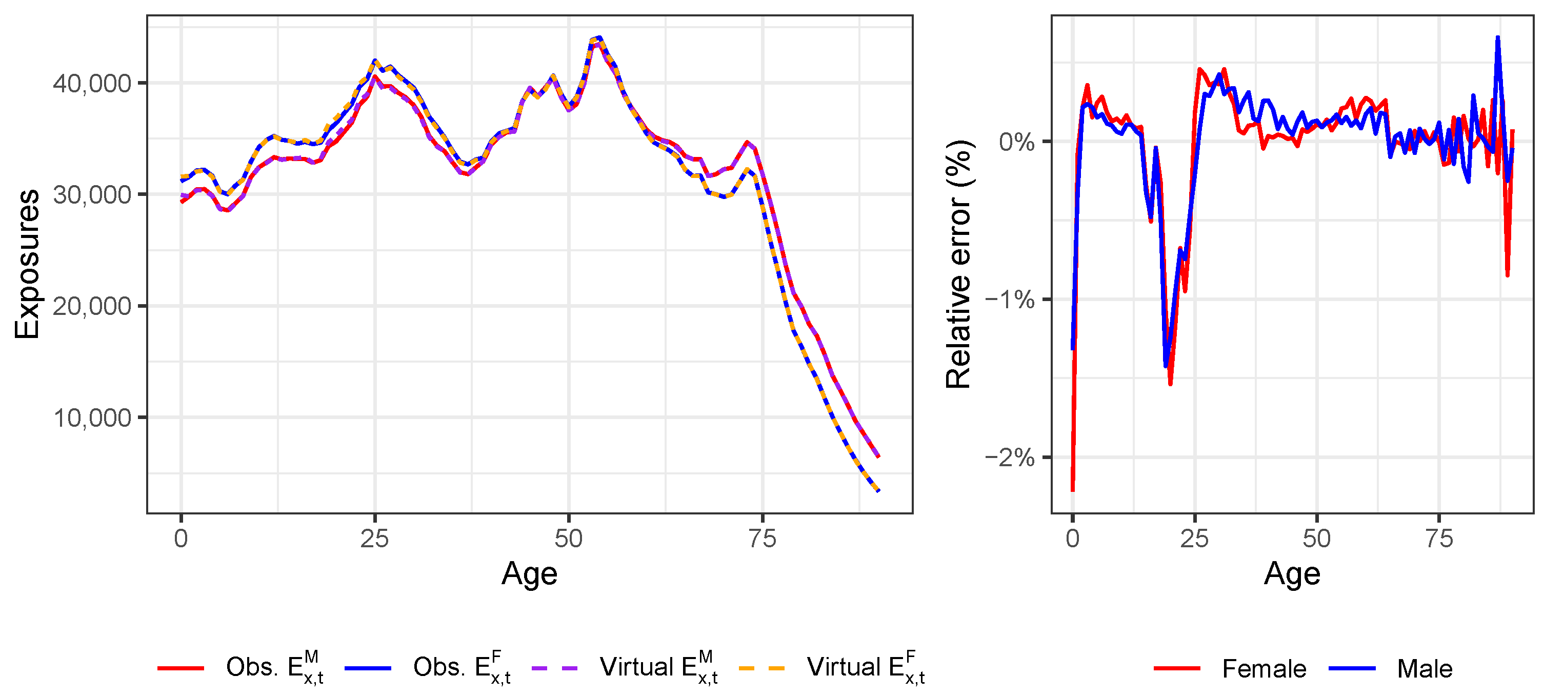
Figure A5 compares the observed Danish, male and female exposures (solid lines) for ages 0–90 in the year 2020 with the virtual exposures (dashed lines) constructed using the protocol. The right panel depicts the relative error between the two exposure curves for males and females. In the case of Denmark, the linear extrapolation of the virtual exposure curve to age 0 does not accurately reflect the observed exposure at age 0. However, for other countries, this extrapolation might perform better, as the pattern over the years 2015–2019 suggests in the case of Belgium (see Figure A1). We also observe a larger spike around the ages 20–25, but the protocol performs quite well overall.
Figure A5.
Validating the protocol to construct virtual exposures in the year 2020 for Denmark from the weekly exposures collected in age buckets from the STMF data series.
Figure A5.
Validating the protocol to construct virtual exposures in the year 2020 for Denmark from the weekly exposures collected in age buckets from the STMF data series.

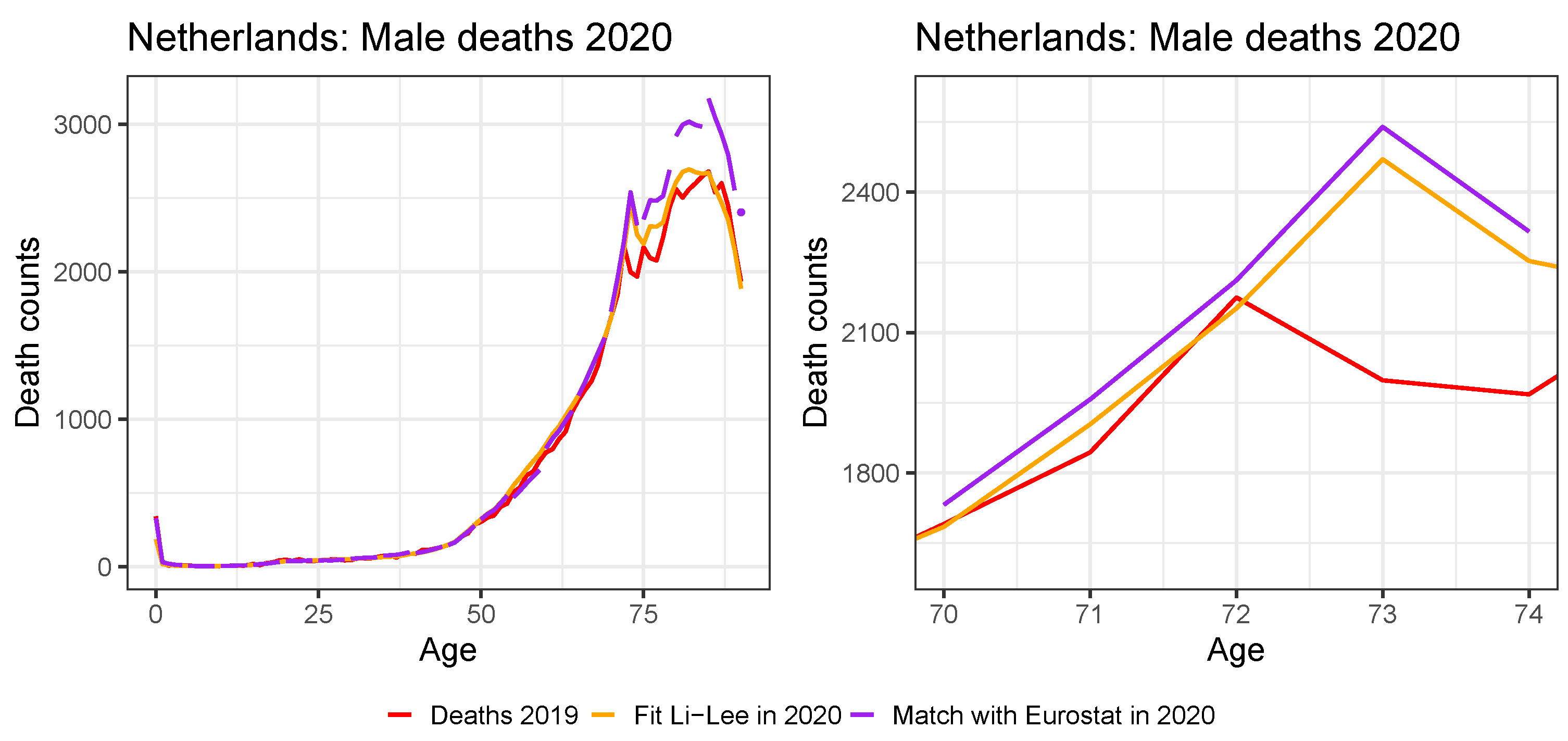
Figure A6 compares the observed Belgian (left) and Danish (right) death counts (solid lines) for ages 0–90 in the year 2020 with the virtual death counts (dashed lines), using the protocol in Appendix C. To construct the virtual death counts, we also use the virtual exposures in the year 2020. The protocol performs quite well, with some deviations for the old ages. The largest difference between the virtual and observed death counts occurs at age 90, since we retrieve information from the open age bucket 90+ in Eurostat to construct .
Figure A6.
Validating the protocol to construct virtual death counts in the year 2020 for Belgium (left) and Denmark (right) from the weekly death counts collected in age buckets from Eurostat.
Figure A6.
Validating the protocol to construct virtual death counts in the year 2020 for Belgium (left) and Denmark (right) from the weekly death counts collected in age buckets from Eurostat.

| 1 | Numbers are retrieved from https://www.statista.com/statistics/1102209/coronavirus-cases-development-europe/ (accessed on 13 December 2021) and https://www.statista.com/statistics/1102288/coronavirus-deaths-development-europe/ (accessed on 13 December 2021) and represent the situation at 5 December 2021. |
| 2 | These numbers of COVID-19 deaths come from the COVID-19 Dashboard by the Center for Systems Science and Engineering (CSSE) at Johns Hopkins University (JHU), see https://www.arcgis.com/apps/opsdashboard/index.html#/bda7594740fd40299423467b48e9ecf6 (accessed on 13 December 2021). |
| 3 | See https://ec.europa.eu/info/live-work-travel-eu/coronavirus-response/safe-covid-19-vaccines-europeans_en (accessed on 21 October 2021) for an overview of the approved, European COVID-19 vaccines and those currently under development, as well as corresponding references. |
| 4 | See https://www.actuaries.org.uk/learn-and-develop/continuous-mortality-investigation/cmi-working-papers/mortality-projections (accessed on 9 November 2021). |
| 5 | This database is our primary database and can be consulted at https://www.mortality.org/ (accessed on 13 April 2021). |
| 6 | Eurostat is the statistical office of the European Union, see https://ec.europa.eu/eurostat (accessed on 13 April 2021). |
| 7 | Statbel is the Belgian statistical office, see https://statbel.fgov.be/en (accessed on 13 April 2021). |
| 8 | This information can be explored using the visualization toolkit on https://mpidr.shinyapps.io/stmortality/ (accessed on 30 July 2021). |
| 9 | Eurostat provides weekly death statistics at https://ec.europa.eu/eurostat/web/COVID-19/data (accessed on 30 July 2021). |
| 10 | The years 1992, 1998, 2004, 2009, 2015 and 2020 contain 53 weeks instead of the usual 52 weeks (ISO 8601 standard). |
| 11 | The HMD team uses a Lee and Carter model to extrapolate recent exposures. The documentation can be consulted via https://www.mortality.org/Public/STMF_DOC/STMFNote.pdf (accessed on 30 July 2021). |
| 12 | See https://appsso.eurostat.ec.europa.eu/nui/show.do?dataset=demo_r_mwk_05&lang=en (accessed on 30 July 2021). |
| 13 | Eurostat only provides weekly death counts for Germany for age buckets of length 10. |
| 14 | We use the nlminb-function in the stats-package of R. |
| 15 | See https://data.worldbank.org/indicator/NY.GDP.PCAP.CD (accessed on 16 June 2021). |
| 16 | See https://www.iso.org/iso-8601-date-and-time-format.html (accessed on 3 November 2021). |
| 17 | The years 1992, 1998, 2004, 2009, 2015 and 2020 contain 53 weeks. |
| 18 | |
| 19 | The case corresponds to the Lee and Miller mortality model as discussed in Lee and Miller (2001). |
| 20 | For all countries except the United Kingdom, we do have the annual exposures at an individual age level in 2019 from either HMD or Eurostat (see Table A1). For Denmark, we already have the annual exposures at an individual age level in the year 2020 available from the HMD. |
| 21 | We use the exposure points and to linearly extrapolate to age 0:
|
| 22 | For all countries except the United Kingdom, we do have the annual death counts at individual ages in 2019 from either HMD or Eurostat (see Table A1). For Belgium and Denmark, we even have the annual death counts at an individual age level in 2020 available from HMD and Statbel, respectively. For these two countries, there is no need to create virtual death counts. |
| 23 | For Belgium and Denmark, we already have the death counts at individual ages in 2020 from Statbel and HMD, respectively. We take the average of both ratios. |
| 24 | We only use the weekly death counts collected in age buckets from Eurostat when they match the reported death counts in the larger age buckets from the STMF data series. We do this for safety reasons because some deviations between the weekly death counts on Eurostat and the STMF data series may occur due to for example territorial differences, e.g., France with or without overseas regions. |
References
- Antonio, Katrien, Anastasios Bardoutsos, and Wilbert Ouburg. 2015. Bayesian poisson log-bilinear models for mortality projections with multiple populations. European Actuarial Journal 5: 245–81. [Google Scholar] [CrossRef]
- Antonio, Katrien, Sander Devriendt, and Jens Robben. 2020. The IA∣BE 2020 Mortality Projection for the Belgian Population. Available online: https://katrienantonio.github.io/papers/report_iabe_2020.pdf (accessed on 24 February 2021).
- Antonio, Katrien, Sander Devriendt, Wouter de Boer, Robert de Vries, Anja De Waegenaere, Hok-Kwan Kan, Egbert Kromme, Wilbert Ouburg, Tim Schulteis, Erica Slagter, and et al. 2017. Producing the Dutch and Belgian mortality projections: A stochastic multi-population standard. European Actuarial Journal 7: 297–336. [Google Scholar] [CrossRef]
- Börger, Matthias, Daniel Fleischer, and Nikita Kuksin. 2014. Modeling the mortality trend under modern solvency regimes. ASTIN Bulletin: The Journal of the IAA 44: 1–38. [Google Scholar] [CrossRef] [Green Version]
- Brouhns, Natacha, Michel Denuit, and Jeroen K. Vermunt. 2002. A Poisson log-bilinear regression approach to the construction of projected lifetables. Insurance: Mathematics and Economics 31: 373–93. [Google Scholar] [CrossRef] [Green Version]
- Cairns, Andrew J. G., David Blake, Kevin Dowd, Guy D. Coughlan, David Epstein, Alen Ong, and Igor Balevich. 2009. A quantitative comparison of stochastic mortality models using data from England and Wales and the United States. North American Actuarial Journal 13: 1–35. [Google Scholar] [CrossRef]
- Chen, Hua, and J. David Cummins. 2010. Longevity bond premiums: The extreme value approach and risk cubic pricing. Insurance: Mathematics and Economics 46: 150–61. [Google Scholar] [CrossRef]
- Chen, Hua, and Samuel H. Cox. 2009. Modeling mortality with jumps: Applications to mortality securitization. The Journal of Risk and Insurance 76: 727–51. [Google Scholar] [CrossRef]
- Cox, Samuel H., Yijia Lin, and Shaun Wang. 2006. Multivariate exponential tilting and pricing implications for mortality securitization. Journal of Risk and Insurance 73: 719–36. [Google Scholar] [CrossRef]
- Gungah, Gavakshi, and Jason Narsoo. 2021. A novel EVT-modified Lee-Carter model for mortality forecasting: An application to extreme mortality events. Journal of Statistics and Management Systems, 1–33. [Google Scholar] [CrossRef]
- Haberman, Steven, and Arthur E. Renshaw. 2011. A comparative study of parametric mortality models. Insurance: Mathematics and Economics 48: 35–55. [Google Scholar] [CrossRef] [Green Version]
- Haberman, Steven, Vladimir Kaishev, Pietro Millossovich, Andrés Villegas, Steven Baxter, Andrew Gaches, Sveinn Gunnlaugsson, and Mario Sison. 2014. Longevity Basis Risk: A Methodology for Assessing Basis Risk. Technical Report. London: Institute and Faculty of Actuaries. [Google Scholar]
- Kannisto, Väinö. 1994. Development of Oldest-Old Mortality, 1950–1990: Evidence from 28 Developed Countries. Odense: Odense University Press. [Google Scholar]
- Koninklijk Actuarieel Genootschap. 2018. Prognosetafel AG2018. Available online: https://www.ag-ai.nl/view/41123-PrognosetafelAG2018.pdf (accessed on 1 November 2020).
- Koninklijk Actuarieel Genootschap. 2020. Prognosetafel AG2020. Available online: https://www.ag-ai.nl/view/45902-PrognosetafelAG2020+%28print%29.pdf (accessed on 1 November 2020).
- Lee, Ronald, and Timothy Miller. 2001. Evaluating the performance of the Lee-Carter method for forecasting mortality. Demography 38: 537–49. [Google Scholar] [CrossRef] [PubMed]
- Lee, Ronald D., and Lawrence R. Carter. 1992. Modeling and forecasting U.S. mortality. Journal of the American Statistical Association 87: 659–71. [Google Scholar] [CrossRef]
- Li, Jackie. 2013. A Poisson common factor model for projecting mortality and life expectancy jointly for females and males. Population Studies: A Journal of Demography 67: 111–26. [Google Scholar] [CrossRef] [PubMed]
- Li, Nan, and Ronald Lee. 2005. Coherent mortality forecasts for a group of populations: An extension of the Lee–Carter method. Demography 42: 575–94. [Google Scholar] [CrossRef] [PubMed] [Green Version]
- Li, Siu-Hang, and Wai-Sum Chan. 2005. Outlier analysis and mortality forecasting: The united kingdom and scandinavian countries. Scandinavian Actuarial Journal 2005: 187–211. [Google Scholar] [CrossRef]
- Liu, Yanxin, and Johnny Siu-Hang Li. 2015. The age pattern of transitory mortality jumps and its impact on the pricing of catastrophic mortality bonds. Insurance: Mathematics and Economics 64: 135–50. [Google Scholar] [CrossRef]
- Pitacco, Ermanno, Michel Denuit, Steven Haberman, and Annamaria Olivieri. 2009. Modeling Longevity Dynamics for Pensions and Annuity Business. London: Oxford University Press. [Google Scholar]
- Rizzi, Silvia, Jutta Gampe, and Paul H. C. Eilers. 2015. Efficient estimation of smooth distributions from coarsely grouped data. American Journal of Epidemiology 182: 138–47. [Google Scholar] [CrossRef] [PubMed] [Green Version]
- Schnürch, Simon, Torsten Kleinow, Ralf Korn, and Andreas Wagner. 2021. The impact of mortality shocks on modeling and insurance valuation as exemplified by COVID-19. Available online: https://papers.ssrn.com/sol3/papers.cfm?abstract_id=3835907 (accessed on 18 June 2021).
- Van Berkum, Frank, Katrien Antonio, and Michel Vellekoop. 2016. The impact of multiple structural changes on mortality predictions. Scandinavian Actuarial Journal 2016: 581–603. [Google Scholar] [CrossRef]
- van Delft, Lotte, and Sarah Huijzer. 2020. Impact of COVID-19 on Dutch Mortality Tables. Available online: https://be.milliman.com/-/media/milliman/pdfs/articles/impact-of-covid-19-on-dutch-mortality-tables.ashx (accessed on 1 November 2020).
- Vanella, Patrizio, Ugofilippo Basellini, and Berit Lange. 2021. Assessing excess mortality in times of pandemics based on principal component analysis of weekly mortality data—The case of COVID-19. Genus 77: 1–36. [Google Scholar] [CrossRef]
- Zhang, Xun, Pu Liao, and Xiaohua Chen. 2021. The negative impact of COVID-19 on life insurers. Frontiers in Public Health 9: 1388. [Google Scholar] [CrossRef] [PubMed]
Figure 1.
Total weekly deaths in Belgium (left), United Kingdom (middle) and Germany (right) in the years 2016–2020 and 2021 (first 27 weeks) for males (top) and females (bottom). Eurostat (Belgium) and STMF (United Kingdom and Germany) data.
Figure 1.
Total weekly deaths in Belgium (left), United Kingdom (middle) and Germany (right) in the years 2016–2020 and 2021 (first 27 weeks) for males (top) and females (bottom). Eurostat (Belgium) and STMF (United Kingdom and Germany) data.

Figure 2.
Stacked male (left) and female (right) exposure for the combined thirteen European countries in 2020 as a function of age. Exposures for the year 2020 are directly available from the HMD for Denmark. However, for Germany, United Kingdom, France, Netherlands, Belgium, Sweden, Austria, Switzerland, Finland, Norway, Luxembourg and Iceland, we transform the weekly exposures collected in age buckets from the STMF data series to exposures at individual ages for the year 2020.

Figure 3.
(Virtual) annual exposures for males (top) and females (bottom) in Belgium (left), the United Kingdom (middle) and Germany (right) as a function of age, years 2015–2020. Exposures for the years 2015–2019 (Belgium), 2015–2018 (United Kingdom) and 2015–2019 (Germany) are directly available from the HMD or Eurostat. However, for the year 2020 (Belgium and Germany) and the years 2019–2020 (United Kingdom), we transform the weekly exposures collected in age buckets from the STMF data series to exposures at individual ages.

Figure 4.
Stacked male (left) and female (right) death counts for the combined thirteen European countries in 2020 as a function of age. Death counts for the year 2020 are directly available from the HMD and Statbel for Denmark and Belgium, respectively. However, for Germany, United Kingdom, France, Netherlands, Sweden, Austria, Switzerland, Finland, Norway, Luxembourg and Iceland, we transform the weekly deaths collected in age buckets from the STMF data series or Eurostat to deaths at individual ages for the year 2020.

Figure 5.
(Virtual) annual death counts for males (top) and females (bottom) in Belgium (left), the United Kingdom (middle) and Germany (right) as a function of age, years 2015-2020. Death counts for the years 2015–2020 (Belgium), 2015–2018 (United Kingdom) and 2015–2019 (Germany) are directly available from the HMD, Eurostat or Statbel. However, for the year 2020 (Germany) and the years 2019–2020 (United Kingdom), we transform the weekly deaths collected in age buckets from the STMF data series or Eurostat to deaths at individual ages.

Figure 6.
The European and Belgium-specific Li and Lee parameters , , , , and for males. The blue line corresponds to the Li and Lee model calibrated on data from the years 1988–2020, with virtually created deaths and exposures for the years 2019–2020. The dark red, dashed line shows the calibrated Li and Lee parameters in the original IA∣BE 2020 model (calibration period 1988–2018(9)).

Figure 7.
The European and Belgium-specific Li and Lee parameters , , , , and for females. The blue line corresponds to the Li and Lee model calibrated on data from the years 1988-2020, with virtually created deaths and exposures for the years 2019–2020. The dark red, dashed line shows the calibrated Li and Lee parameters in the original IA∣BE 2020 model (calibration period 1988–2018(9)).

Figure 8.
Projection of the calibrated time dependent parameters in the Li and Lee model: (top) and (bottom). Male (left) and female (right) data, calibration period 1988–2020, projection period 2021–2070, method of Section 5.1. We show the , median (white lines) and quantile, based on 10,000 simulations across each weighting scenario. The black lines visualize the calibrated period effects: and .

Figure 9.
Estimated and projected Belgian mortality rates . Male data, ages 25, 45 (top) and 65, 85 (bottom), calibration period 1988–2020, projection period 2021–2070, method of Section 5.1. We show the , median (white lines) and quantile, based on 10,000 simulations across each weighting scenario. The blue dots and the black lines represent the observed and fitted mortality rates, respectively. The dark red, dashed line shows the calibrated mortality rates and the median quantile of the simulations in the original IA∣BE 2020 model.

Figure 10.
Estimated and projected period life expectancies for Belgium. Male (top) and female (bottom) data, ages 0 (left) and 65 (right), calibration period 1988–2020, projection period 2021–2070, method of Section 5.1. We show the , median (white lines) and quantile (fan charts), based on 10,000 simulations, across each weighting scenario. The dark red, dashed line shows the quantile originating from the original IA∣BE 2020 model. The blue dots and black line represent the observed and fitted period life expectancies, respectively.

Figure 11.
The European and Belgian parameters , , , , and in the adjusted Lee and Miller mortality model for males. The coloured lines correspond to the different weighting scenarios in the calibration set-up. The mortality model is calibrated on data from 1988 to 2020 and contains virtually created deaths and exposures for the years 2019–2020.

Figure 12.
The European and Belgian parameters , , , , and in the adjusted Lee and Miller mortality model for females. The coloured lines correspond to the different weighting scenarios in the calibration set-up. The mortality model is calibrated on data from 1988 to 2020 and contains virtually created deaths and exposures for the years 2019–2020.

Figure 13.
Projection of the calibrated time dependent parameters in the adjusted Lee and Miller model: (top) and (bottom). Male (left) and female (right) data, calibration period 1988–2020 and projection period 2021–2070, method of Section 5.2. We show the , median (white lines) and quantile, based on 10,000 simulations across each weighting scenario. The coloured, solid lines visualize the calibrated period effects for each weighting scenario: and . white space white space white space white space white space white space white.

Figure 14.
Estimated and projected Belgian mortality rates . Male data, ages 25, 45 (top) and 65, 85 (bottom), calibration period 1988–2020, projection period 2021–2070, method of Section 5.2. We show the , median (white lines) and quantile (fan charts), based on 10,000 simulations across each weighting scenario. The blue dots and the coloured, solid lines represent the observed and fitted mortality rates, respectively. The dark red, dashed line shows the calibrated mortality rates and the median quantile of simulations in the original IA∣BE 2020 model.

Figure 15.
Estimated and projected period life expectancies for Belgium. Male (top) and female (bottom) data, ages 0 (left) and 65 (right), calibration period 1988–2020, projection period 2021–2070. Calibration and projection is based on the method in Section 5.1. We show the quantile, median (white lines) and quantile (fan charts), based on 10,000 simulations, across each weighting scenario. The dark red, dashed line shows the quantile originating from the original IA∣BE 2020 model. The blue dots represent the observed period life expectancies.

Table 1.
Time series parameter estimates, male and female data, ages 0–90, years 1988–2020, Section 5.1.
Table 1.
Time series parameter estimates, male and female data, ages 0–90, years 1988–2020, Section 5.1.
| Weight 2020 | ||||||
|---|---|---|---|---|---|---|
| 0 | −0.2315 | −0.1938 | 0.0071 | −0.0091 | 0.9027 | 0.9033 |
| 0.25 | −0.2236 | −0.1872 | 0.0025 | −0.0142 | 0.9306 | 0.9600 |
| 0.50 | −0.2159 | −0.1807 | −0.0028 | −0.0180 | 0.9424 | 0.9730 |
| 0.75 | −0.2083 | −0.1743 | −0.0083 | −0.0216 | 0.9487 | 0.9790 |
| 1 | −0.2009 | −0.1681 | −0.0138 | −0.0250 | 0.9527 | 0.9825 |
| IA∣BE 2020 | −0.2285 | −0.1882 | 0.0140 | −0.0240 | 0.9682 | 0.9226 |
Table 2.
The cohort life expectancy for a 0 and 65 year old in 2020. The , median and quantile obtained from 10,000 simulations are shown, for males and females. We obtain the best-estimate of the cohort life expectancy by taking the zero vector for the noise terms in Equation (4) to project the time dependent parameters.
| Cohort Life Expectancy in 2020 | Males | Females | |||
|---|---|---|---|---|---|
| 0 | 65 | 0 | 65 | ||
| Recalibration 2020 weight = 0 | Best. Est. | 89.36 | 19.70 | 91.42 | 22.78 |
| Recalibration 2020 weight = 0.25 | Best. Est. | 89.07 | 19.65 | 91.11 | 22.65 |
| Recalibration 2020 weight = 0.50 | Best. Est. | 88.77 | 19.58 | 90.78 | 22.56 |
| Recalibration 2020 weight = 0.75 | Best. Est. | 88.45 | 19.52 | 90.46 | 22.48 |
| Recalibration 2020 weight = 1 | Best. Est. | 88.13 | 19.45 | 90.13 | 22.41 |
| IA∣BE 2020 | Best. Est. | 89.91 | 20.38 | 91.54 | 23.14 |
Table 3.
Time series parameter estimates, male and female data, ages 0–90, years 1988–2020, Section 5.2.
Table 3.
Time series parameter estimates, male and female data, ages 0–90, years 1988–2020, Section 5.2.
| Weight 2020 | ||||||
|---|---|---|---|---|---|---|
| 0 | −0.2177 | −0.1881 | −0.0474 | −0.0300 | 0.9588 | 0.9124 |
| 0.25 | −0.2139 | −0.1836 | −0.0305 | −0.0277 | 0.9545 | 0.9607 |
| 0.50 | −0.2094 | −0.1809 | −0.0319 | −0.0303 | 0.9243 | 0.8567 |
| 0.75 | −0.2061 | −0.1791 | −0.0424 | −0.0337 | 0.8539 | 0.7110 |
| 1 | −0.2037 | −0.1774 | −0.0587 | −0.0324 | 0.8248 | 0.5297 |
Table 4.
The cohort life expectancy for a 0 and 65 year old in 2020. The quantile, median and quantile obtained from 10,000 simulations are shown, for males and females. We obtain the best-estimate of the cohort life expectancy by taking the zero vector for the noise terms in Equation (4) to project the time dependent parameters.
| Cohort Life Expectancy in 2020 | Males | Females | |||
|---|---|---|---|---|---|
| 0 | 65 | 0 | 65 | ||
| Recalibration 2020 weight = 0 | Best. Est. | 89.95 | 20.31 | 92.15 | 23.32 |
| Recalibration 2020 weight = 0.25 | Best. Est. | 89.25 | 19.89 | 91.58 | 22.99 |
| Recalibration 2020 weight = 0.50 | Best. Est. | 88.60 | 19.57 | 91.12 | 22.82 |
| Recalibration 2020 weight = 0.75 | Best. Est. | 88.05 | 19.37 | 90.71 | 22.71 |
| Recalibration 2020 weight = 1 | Best. Est. | 87.57 | 19.19 | 90.32 | 22.58 |
| IA∣BE 2020 | Best. Est. | 89.91 | 20.38 | 91.54 | 23.14 |
Publisher’s Note: MDPI stays neutral with regard to jurisdictional claims in published maps and institutional affiliations. |
© 2022 by the authors. Licensee MDPI, Basel, Switzerland. This article is an open access article distributed under the terms and conditions of the Creative Commons Attribution (CC BY) license (https://creativecommons.org/licenses/by/4.0/).
Share and Cite
MDPI and ACS Style
Robben, J.; Antonio, K.; Devriendt, S. Assessing the Impact of the COVID-19 Shock on a Stochastic Multi-Population Mortality Model. Risks 2022, 10, 26. https://doi.org/10.3390/risks10020026
AMA Style
Robben J, Antonio K, Devriendt S. Assessing the Impact of the COVID-19 Shock on a Stochastic Multi-Population Mortality Model. Risks. 2022; 10(2):26. https://doi.org/10.3390/risks10020026
Chicago/Turabian StyleRobben, Jens, Katrien Antonio, and Sander Devriendt. 2022. "Assessing the Impact of the COVID-19 Shock on a Stochastic Multi-Population Mortality Model" Risks 10, no. 2: 26. https://doi.org/10.3390/risks10020026
Note that from the first issue of 2016, this journal uses article numbers instead of page numbers. See further details here.