Epidemiological Model With Anomalous Kinetics: Early Stages of the COVID-19 Pandemic

1 Introduction

The classic and still widely used SIR and SEIR epidemiological models [1] represent contagion and removal in analogy with the law of mass action in chemistry, corresponding to a mean-field approach based on the assumption of homogeneous mixing. The latter hypothesis constitutes an oversimplification, particularly for the COVID-19 pandemic, due to strong government intervention (social distancing; lockdown) and underreporting as the number of cases grows beyond testing capacity. Diverse aspects are discussed, assuming homogeneous or nonhomogeneous mixing, in epidemiological models in general [2–4], as well as in the current pandemic [5–15].

Epidemic models can be formulated on varying levels of detail, from individual agents in geographically realistic settings to models of large populations without spatial structure. Each level has its own benefits and costs; the study of an ensemble of models is expected to yield a more reliable description than any single approach in isolation. In chemical kinetics of processes involving anomalous diffusion and/or complex conformational pathways, effective descriptions typically employ noninteger power-law terms where the mean-field or mass-action analysis involves integer powers of concentrations, as in the analysis of reassociation of folded proteins [16, 17]. With this motivation, we consider SIR- and SEIR-like models in which the contagion and removal terms depend on $I^{q_{up}}$ and $I^{q_{down}}$, respectively, instead of depending linearly on I, as they do in mean-field/homogeneous descriptions. Such generalization is consistent with anomalous human mobility and spatial disease dynamics [18, 19] and emerges naturally within statistical mechanics based on nonadditive entropies [20] as we show in what comes next.

Let us now follow along lines close to [16], which provided a satisfactory description of reassociation in folded proteins [17]. Consider the equation

Its solution is given by

with $e_q^z\equiv {[1+\left(1-q\right)z]}^{1/\left(1-q\right)}\left(e_1^z=e^z\right)$, a function that emerges naturally in the nonadditive-entropy-based statistical mechanics [20]. We have a monotonically increasing function $y\left(t\right)$ for $a>0$ (with infinite support if $q\le 1$ and finite support if $q>1$) and a monotonically decreasing function for $a<0$ (with infinite support if $q\ge 1$ and finite support if $q<1$). Notice an important point that will permeate through this entire paper: if $q=1$, only then the coefficient a (which characterizes the scale of the evolution of $y\left(t\right)/y\left(0\right)$ with time) is not renormalized by the initial condition $y\left(0\right)$. If $q\ne 1$, the effective constant $\left\{a{\left[y\left(0\right)\right]}^{q-1}\right\}$ will differ from a; the difference can be very important depending on the values of q and $y\left(0\right)$.

2 Generalized Models

2.1 q-SIR Model

The SIR set of equations is (see [1] for instance) as follows:

with $\beta >0$, $\gamma >0$, and $S+I+R=N=constant$, N is the total population, $S\equiv susceptible$, $I\equiv infected$, and $R\equiv removed$ (removed means either recovered or dead). Now let us q-generalize this model as follows:

with $q_{up}\le 1$ and $q_{down}\ge 1$, where the bilinear term is generalized into a nonbilinear one and the effective population $N_{eff}=\rho N$ with $\rho \le 1$. These equations generically have a single peak for $I\left(t\right)$. In all cases, we have $S\left(t\right)+I\left(t\right)+R\left(t\right)=N_{eff}$; moreover, $0\le S\left(t\right)/N_{eff}$, $I\left(t\right)/N_{eff}$, and $R\left(t\right)/N_{eff}\le 1$. Consistently, in the set of Eq. 4, it is enough to retain the first two. Let us qualitatively compare the SIR and q-SIR models given by Eqs 3 and 4, respectively, by focusing on the β term; i.e., let us compare ${\beta }_{SIR}\left[S\left(t\right)/N][I\left(t\right)/N\right]$ with ${\beta }_{qSIR}{[S\left(t\right)/N_{eff}][I\left(t\right)/N_{eff}]}^{q_{up}}=\frac{{\beta }_{qSIR}}{{[I\left(t\right)/N_{eff}]}^{1-q_{up}}}\left[S\left(t\right)/N_{eff}][I\left(t\right)/N_{eff}\right]$; we remind that $\rho =1$ yields $N_{eff}=N$. It follows that roughly ${\beta }_{SIR}\simeq \frac{{\beta }_{qSIR}}{\left[I\left(t\right)/N_{eff}\right)}$. Since, before the peak, $I\left(t\right)$ steadily increases with time, a fixed value for $\left(1-q_{up}\right)>0$ acts qualitatively as a phenomenological time-dependent ${\beta }_{SIR}\left(t\right)$ which decreases with time. These tendencies are similarly realistic since they both reflect, each in its own manner, the generic action of pandemic authorities to isolate people in order to decrease the contagion represented by the β term in both models.

The particular limit $R\left(t\right)\equiv 0$ (hence $S\left(t\right)+I\left(t\right)=N_{eff}$) in Eq. (4) yields $I\left(t\right)=I\left(0\right)e_{q_{down}}^{-\gamma {[I\left(0\right)/N_{eff}]}^{q_{down}-1}t}$ if $\beta =0$, and $I\left(t\right)=\frac{I\left(0\right)e^{\beta t}}{\left(I\left(0\right)/N_{eff}\right)e^{\beta t}+\left[1-I\left(0\right)/N_{eff}\right]}$ if $\left(\gamma ,q_{up}\right)=\left(\mathrm{0,1}\right)$. For generic $q_{up}<1$ and $R\left(t\right)\equiv 0$, Eq. (4) yields

and hence,

where $\text{Γ}$ is the Gamma function and $\tilde{F}$ is the regularized hypergeometric function. As an illustration, let us consider $q_{up}=1/2$. It follows $\text{ln}\left[\frac{1-\sqrt{1-S/N_{eff}}}{1+\sqrt{1-S/N_{eff}}}\times \frac{1+\sqrt{1-S\left(0\right)/N_{eff}}}{1-\sqrt{1-S\left(0\right)/N_{eff}}}\right]=-\beta t$; hence,

Before the peak, $I\left(t\right)$ increases nearly exponentially if $q_{up}=1$ and is roughly characterized by $I\left(t\right)\simeq t^{\frac{1}{1-q_{up}}}$ if $q_{up}<1$. After the peak, $I\left(t\right)$ decreases exponentially if $q_{down}=1$ and is roughly characterized by $I\left(t\right)\simeq t^{-\frac{1}{q_{down}-1}}$ if $q_{down}>1$. These various aspects are illustrated in Figure 1. An important remark is necessary at this point. The possibility for nonbilinear coupling $\beta \left(S/N_{eff}\right){\left(I/N_{eff}\right)}^{q_{up}}$ between subpopulations seems quite natural since nonhomogeneous mixing involves complex dynamics and networks for the susceptible and infected people, as well as for the infecting agent of the disease. But why would it be necessary to also allow, at the present phenomenological level, a nonlinear behavior for the one-subpopulation term $\gamma {\left(I/N_{eff}\right)}^{q_{down}}$ itself? The answer might be found in nontrivial (multi)fractal-path-like relaxation mechanisms such as the one that is known to happen in reassociations in folded proteins [16, 17].

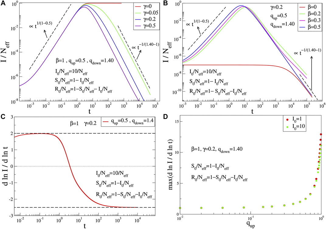
FIGURE 1. Time evolution of $I\left(t\right)$ for the q-SIR equations with $N_{eff}={10}^8$; we consider t to run virtually from zero to infinity (not necessarily during only the typical range of real epidemics, say 1,000 days). (A) Fixed β and various values of γ. For $\gamma =0$ and $\forall \beta$, $I\left(t\right)/N_{eff}$ precisely recovers the expression given in Eq. (6). The slope at the first inflection point for increasing time is given by $max\left[d\text{ln}I/d\text{ln}t\right]=1/\left(1-q_{up}\right)$, $\forall \gamma$. (B) Fixed γ and various values of β. For $\beta =0$, the q_down-exponential function is precisely recovered. (C) Time dependence of the slope of $\left[d\text{ln}\left(I/N_{eff}\right)/d\text{ln}t\right]$, which appears to be bounded between $1/\left(1-q_{up}\right)$ ($=2$ in this example) and $-1/\left(q_{down}-1\right)$ ($=-2.5$ in this example) (dashed lines). The dotted line corresponds to the position of the peak of $I\left(t\right)$, and the maximum (minimum) corresponds to the left (right) inflection point. (D) The maximal slope of $I\left(t\right)/N_{eff}$ as a function of $q_{up}$. The high value at $q_{up}=1$ reflects the divergence expected in the limit $q_{up}=q_{down}=1$. Indeed, in this limit, the present q-SIR model recovers the standard SIR model, which increases exponentially (and not as a power-law) toward the corresponding peak. Notice also that this slope decreases when $I_0/N_{eff}$ increases.

We have checked that the q-SIR model provides functions $I\left(t\right)$ that are numerically close but different from the quite performing ansatz in [5], namely, $I\left(t\right)\propto t^{\overline{\alpha }}{e}_{\overline{q}}^{-\overline{\beta }{t}^{\overline{\gamma }}}$, whose behavior before and after the peak is, respectively, $t^{\overline{\alpha }}$ and $t^{\overline{\alpha }-\overline{\gamma }/\left(\overline{q}-1\right)}$. Still, both approaches have power-law behaviors before and after the peak. We also checked $I\left(t\right)\propto e_{q_{up}}^{{\beta }_{up}t}\times e_{q_{down}}^{-{\beta }_{down}t}$, and the results are once again numerically close but nevertheless different from the ansatz in [5].

2.2 q-SEIR Model

The q-SIR model is not capable (for any choice of its parameters) of correctly fitting the epidemiologically crucial function $I\left(t\right)$ for the COVID-19 available data for various countries. Since this generalization of the simplest model does not provide a useful tool for COVID-19 data, we addressed a more sophisticated one, namely, a four-compartment model known as SEIR. Therefore, we next q-generalize the SEIR model with no vital dynamics (no births; no deaths), which is given by

with $S+E+I+R=N$, where E stands for exposed. We can generalize it as follows:

where once again we have generalized the bilinear couplings between subpopulations into nonbilinear ones and the linear $\gamma I$ term into a nonlinear one. Its particular instance $E\left(t\right)\equiv 0$ (hence, $S\left(t\right)+I\left(t\right)+R\left(t\right)=N_{eff}$) precisely recovers the q-SIR model, as defined here above. Notice that the cumulative function$C\left(t\right)$ of $I\left(t\right)$ is given by $C\left(t\right)\equiv {{\displaystyle \int }}_0^{t}d{t}^{\prime }I\left(t^{\prime }\right)={{\displaystyle \int }}_0^{t}d{t}^{\prime }{\left[\frac{1}{\gamma }\frac{dR\left(t^{\prime }\right)}{d{t}^{\prime }}\right]}^{1/q_{down}}$, which differs from the expression $C\left(t\right)=R\left(t\right)$ currently used in the SEIR model. It is of course possible to further generalize the above q-SEIR set of four equations by allowing in the right hand $S^{q_s}$ (with $q_s\ne 1$) instead of S and $E^{q_{\mathit{ϵ}}}$ (with $q_{\mathit{ϵ}}\ne 1$) instead of E, but no need has emerged to increase the number of free parameters of the model, since the allowance for $q_{up}<1$ and for $q_{down}>1$ appears to be enough for satisfactorily reproducing all the relevant features of the COVID-19 available data. Indeed, the variable which is epidemiologically crucial for avoiding a medical-hospital collapse in a given region is $I\left(t\right)$, and this time dependence generically appears to be very satisfactorily described by just allowing the possibility for $q_{up}\ne 1$ and/or $q_{down}\ne 1$. Notice that $\beta {\left(I/N_{eff}\right)}^{q_{up}}$ is a convex function of $\left(I/N_{eff}\right)$ for $0<q_{up}<1$ and $\gamma {\left(I/N_{eff}\right)}^{q_{down}}$ is a concave function of $\left(I/N_{eff}\right)$ for $q_{down}>1$. These tendencies, illustrated in Figure 2, as well as the numerical values for the various coefficients of the model, are in agreement with the available medical/epidemiological evidence [21–25]. Notice also that, through $\tau \equiv \gamma t$ and $\left(\overline{I}/N_{eff}\right)\equiv {\left(I/N_{eff}\right)}^{q_{down}}$, we can eliminate, without loss of generality, two fitting parameters (e.g., γ and $q_{down}$) within the set of equations (8). Finally notice that if we consider $\beta =\sigma =0$, we precisely recover Eq. (1) and its analytical solution in Eq. (2). Therefore, even if the general analytical solution of the set of equations (8) is not available (due to mathematical intractability), the initial conditions naturally renormalize (in a nontrivial manner) the coefficients $\left(\beta ,\sigma ,\gamma \right)$ of the model, and the effective population $N_{eff}$ becomes a fitting parameter of the model. These renormalizations disappear of course if $q_{up}=q_{down}=1$, i.e., for the standard SEIR model; concomitantly $N_{eff}$ ($=\rho N$, with $\rho \le 1$) ceases being a fitting parameter and can be directly taken from the actual population N of the particular region under focus. For other mathematical aspects of nonlinear models such as the present one, the reader may refer to [26].

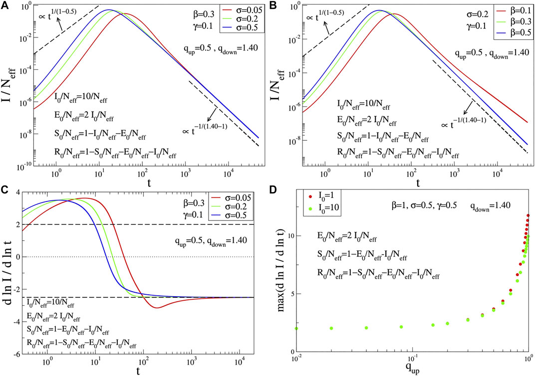
FIGURE 2. Time evolution of $I\left(t\right)$ for the q-SEIR equations with $N_{eff}={10}^8$; we consider t to run virtually from zero to infinity (not necessarily during only the typical range of real epidemics, say 1,000 days). (A) Fixed $\left(\beta ,\gamma \right)$ and various values of σ. (B) Fixed $\left(\sigma ,\gamma \right)$ and various values of β. (C) Time dependence of the slope of $\left[d\text{ln}I/d\text{ln}t\right]$, which, in contrast with the q-SIR equations, is not bounded between $1/\left(1-q_{up}\right)>0$ and $-1/\left(q_{down}-1\right)<0$ (dashed lines). The dotted line corresponds to the position of the peak of $I\left(t\right)$, and the maximum (minimum) corresponds to left (right) inflection points. (D) The maximal slope of $I\left(t\right)/N_{eff}$ as a function of $q_{up}$. The high value at $q_{up}=1$ reflects the divergence expected in the limit $q_{up}=q_{down}=1$. Indeed, in this limit, the present q-SEIR model recovers the standard SEIR model, which increases exponentially (and not as a power-law) toward the corresponding peak. Notice also that this slope decreases when $I_0/N_{eff}$ increases.

3 Application of q-SEIR Model to COVID-19 Pandemic

In Figures 3 and 4, we have illustrations of this model for realistic COVID-19 cases. We identify the present variable I with the number of active cases,¹ as regularly updated online [27]. We verify that the description provided by the q-SEIR model for nonhomogeneous epidemiological mixing is indeed quite satisfactory for the early stages of the pandemic (before an unpredictable but possible second wave). Let us also mention that we have not followed here a road looking for the minimal number of free parameters, but rather a road where various realistic elements are taken into account, even if at the fitting-parameter level some of them might be redundant. Any further model yielding a deeper, or even first-principle, expression of exponents such as $q_{up}$ and $q_{down}$ in terms of microscopic/mesoscopic mechanisms is very welcome. This is by no means a trivial enterprise but, if successfully implemented, this would probably follow a road analogous to anomalous diffusion, namely, from Fourier’s heat equation through Muskat’s Porous Medium Equation [28] to Plastino and Plastino nonlinear Fokker-Planck equation [29], which in turn implied the scaling law $\overline{\alpha }=2/\left(3-q\right)$ [30] ($\overline{\alpha }$ being defined through the scaling between $x^2$ and $t^{\overline{\alpha }}$ and q being the index value of the q-Gaussian solution for the nonlinear Fokker-Planck equation). This scaling law recovers, for $q=1$, the Brownian motion scaling $\langle x^2\rangle \propto t$ and was impressively validated within 2% error in granular matter [31]. This phenomenological line was later legitimated on the basis of microscopic overdamped mechanisms in at least a wide class of systems, namely, providing $q=0$ for the motion of vortices in type-II superconductors [32], and later extended to D-dimensional $1/r^{\lambda }$ short-range repulsive interactions ($\lambda /D\ge 1$), leading to $q=1-\lambda /D$ [33]. These approaches were shown to satisfy the zeroth law of thermodynamics, an H-theorem, and Carnot’s cycle efficiency, with microscopically established analytical equations of state [34–37]. An attempt to follow along similar lines for the present q-SEIR model would surely be a very interesting challenge. In summary, we have q-generalized, through Eq. (8), the SEIR epidemiological model. By solving this set of deterministic equations given the initial conditions and its parameters, we obtain $[S\left(t\right),E\left(t\right),I\left(t\right)]$, as well as the cumulative function $C\left(t\right)$. We have focused on $I\left(t\right)$ because the hardest quantities for satisfactorily fitting are the number of active cases and that of deaths and also because those are the most crucial quantities for making correct sanitary and epidemiological decisions.

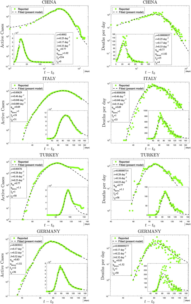
FIGURE 3. Time evolution of available data for COVID-19 numbers of active cases (probably under-reported in most cases) and deaths per day [27] and their (linear scale) Least Squares Method fittings with $N_{eff}I\left(t\right)$ from the q-SEIR model; $\rho =N_{eff}/N$, where N is the population of the country. Notice that, (i) by convention, $t_0=0$ for China; (ii) parameters such as $\rho N$ are particularly relevant for sanitary-epidemiological decisions, and, as it is natural, $\rho \left(deaths\right)\ll \rho \left(active\right)$ for any given country; (iii) for any given country, the values of $\left(q_{up},q_{down}\right)$ are the same for both curves of active cases and of deaths; (iv) the dates of the peaks of the active cases and deaths per day do not necessarily coincide; (v) the values that emerge for $\beta /\gamma$ (reproduction number or growth rate), $1/\beta$ (exposition time), $1/\gamma$ (recovering time), and $1/\sigma$ (incubation time) are consistent with those currently indicated in the literature [21–25]; (vi) we considered all the data reported until June 13, excluding some very initial transients or sudden anomalous discrepancies (e.g., in China, Turkey, and Brazil).

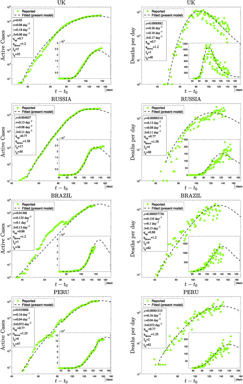
FIGURE 4. Continuation of Figure 3.

From a general perspective, let us stress that the law of mass action, the Arrhenius relaxation law, and the Kramers mechanism [38] of escape over a barrier through normal diffusion constitute pillars of contemporary chemistry. They are consistent with Boltzmann-Gibbs (BG) statistical mechanics and constitute some of its important successes. However, they need to be modified when the system exhibits complexity due to hierarchical space and/or time structures. It is along this line that a generalization has been proposed based on nonadditive entropies [20], characterized by the index q ($q=1$ recovers the BG frame): see, for instance, [16, 39–43]. It is along these same lines that lies the present q-generalization of the standard SEIR model.

At the level of the numerical performance of the present q-SEIR model for the COVID-19 pandemic, it advantageously compares with models including time-dependent coefficients [44–47]. For instance, the SEIQRDP model [44, 45, 47] includes seven equations with several coefficients, two of them phenomenologically being time-dependent. It does fit rather well the COVID-19 reported data until a given date. However, the q-SEIR, which includes four (instead of seven) equations with several coefficients, all of them being fixed in time, fits definitively better the same data for all the countries that we have checked: see illustrations in Figure 5.

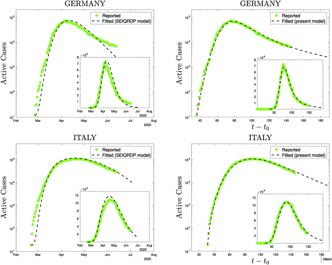
FIGURE 5. Comparison, using precisely the same reported data (green dots), of the SEIQRDP model (left plots) and the q-SEIR model (right plots) for the time series of Germany (from February 26^th to June 13^th 2020) and of Italy (from February 21^st to June 13^th 2020). To obtain the SEIQRDP fittings (seven linear/bilinear equations satisfying $S+E+I+Q+R+D+P=N$ and including several fixed as well as two time-dependent coefficients), we have used the online program [47]. To obtain the q-SEIR fittings (four not necessarily linear/bilinear equations satisfying $S+E+I+R=N_{eff}$ and including only fixed parameters, two of them being the nonlinear exponents $q_{up}$ and $q_{down}$), we have used a Standard Least Squares Method (linear scales).

At this stage, let us emphasize a rather interesting fact. Neither the SIR nor the SEIR models distinguish the dead from the recovered, within the removed (R) subpopulation. However, the same values for $\left(q_{up},q_{down}\right)$ fit satisfactorily both the numbers of active cases and of deaths per day for a given country, as shown in Figures 3 and 4. At this point, it would be worth noting that although the present model, unlike, for example, the SEIRD model [48, 49], does not distinguish deaths from healings, the deceased cases will still be roughly proportional to infected people. It is this proportionality, we believe, which makes us obtain reasonable fits using the variable I of the model, again incorporating the proportionality into $N_{eff}$ and hence into ρ. It is also evident from these figures that the data for deaths per day are more scattered than those for active cases. This is due to the fact that the real data for the former are much less than for the latter. This is also the reason for the significantly small ρ values of deaths per day compared to those of active cases.

4 Conclusion

To conclude, let us remind that the q-SEIR model recovers, as particular instances, the q-SIR model introduced here, as well as the traditional SEIR and SIR ones. It has, however, an important mathematical difference with the usual epidemiological models. Virtually all these models (SIR, SEIR, SAIR, SEAIR, SIRASD, SEAUCR, and SEIQRDP) are defined through equations that are multilinear in their variables; i.e., that are linear in each one of its variables. This multilinearity disappears in models such as the present q-SIR and q-SEIR ones if either $q_{up}$ or $q_{down}$ differs from unity. Consequently $N_{eff}$ definitively plays a different role since it sensibly enters within the set of fitting parameters of the q-generalized models; its precise interpretation remains to be elucidated, perhaps in terms of the sociogeographical circumstances of that particular region. Last but not least, let us stress that the aim of the present q-SEIR model is to mesoscopically describe a single epidemiological peak, including its realistic power-law growth and relaxation in the time evolution of the number of active cases, and by no means to qualitatively address possibilities such as the emergence of two or more peaks, a task which is (sort of naturally, but possibly less justified on fundamental grounds) attainable within approaches using traditional (multilinear) models where one or more coefficients are allowed to phenomenologically depend on time by realistically adjusting their evolution along the actual epidemics. Alternatively, it is always possible to approach the two-peak case by proposing a linear combination of two q-SEIR curves starting each of them at two different values of the departing time ($t_0$).

Data Availability Statement

The datasets presented in this study can be found in online repositories. The names of the repository/repositories and accession number(s) can be found below: https://data.humdata.org/dataset/novel-coronavirus-2019-ncov-cases

Author Contributions

All authors contributed equally to the article.

Conflict of Interest

The authors declare that the research was conducted in the absence of any commercial or financial relationships that could be construed as a potential conflict of interest.

Acknowledgments

We have greatly benefitted from very fruitful discussions with R. Dickman, T. Pereira and D. Eroglu, as well as from partial financial support by CNPq and Faperj (Brazilian agencies).

Footnotes

¹At this point, it should be noted that the variable I in the model represents both detected plus undetected active cases although, of course, the database includes only detected ones as active cases. However, since these cases are roughly proportional to each other (with a proportionality coefficient which might change from country to country), we use the model variable I to fit the active cases reflecting the incorporation of this proportionality into $N_{eff}$ and hence into ρ.

References

1. Daley DJ, Gani JM. Epidemic modelling: an introduction. Cambridge: Cambridge University Press (1999).
Google Scholar
2. Bansal S, Grenfell BT, Meyers LA. When individual behaviour matters: homogeneous and network models in epidemiology. J R Soc Interface (2007) 4:879. doi:10.1098/rsif.2007.1100
PubMed Abstract | CrossRef Full Text | Google Scholar
3. Burr TL, Chowell G. Signatures of non-homogeneous mixing in disease outbreaks, Math Comput Model (2008) 48:122. doi:10.1016/j.mcm.2007.09.009
CrossRef Full Text | Google Scholar
4. Milwid RM, O’Sullivan TL, Poljak Z, Laskowski M, Greer AL. Comparing the effects of non- homogenous mixing patterns on epidemiological outcomes in equine populations: a mathematical modelling study, Sci Rep (2019) 9:3227. doi:10.1038/s41598-019-40151-2
5. Tsallis C, Tirnakli U. Predicting COVID-19 peaks around the world. Front Phys (2020) 8, 217. doi:10.3389/fphy.2020.00217
6. Sebastiani G, Massa M, Riboli E. COVID-19 epidemic in Italy: evolution, projections and impact of government measures. Eur J Epidemiol (2020) 35:341. doi:10.1007/s10654-020-00631-6
7. Chowdhury R, Heng K, Shawon MSR, Goh G, Okonofua D, Ochoa-Rosales C, et al. Dynamic interventions to control COVID-19 pandemic: a multivariate prediction modelling study comparing 16 worldwide countries, Eur J Epidemiol (2020) 35:389. doi:10.1007/s10654-020-00649-w
8. Wang L, Chen H, Qiu S, Song H, Evaluation of control measures for COVID-19 in Wuhan, China. J Infect (2020) 81:318. doi:10.1016/j.jinf.2020.03.043
9. Manchein C, Brugnago EL, da Silva RM, Mendes CFO, Beims MW. Strong correlations between power-law growth of COVID-19 in four continents and the inefficiency of soft quarantine strategies, Chaos (2020) 30:041102. doi:10.1063/5.0009454
10. Ashurov R, Umarov S. Determination of the order of fractional derivative for subdiffusion equation. arxiv 13468 (2020).
11. Ziff AL, Ziff RM, et al. Fractal kinetics of COVID-19 pandemic (with update 3/1/20) medRxiv preprint (2020). doi:10.1101/2020.02.16.20023820
12. Vasconcelos GL, Macedo AMS, Ospina R, Almeida FAG, Duarte-Filho GC, Brum AA, et al. Modelling fatality curves of COVID-19 and the effectiveness of intervention strategies. PeerJ (2020) 8:e9421. doi:10.7717/peerj.9421
13. Curado EMF, Curado MR. A discrete-time-evolution model to forecast progress of COVID-19 outbreak. PLoS ONE (2020) 15:e0241472. doi:10.1371/journal.pone.0241472
14. Costa GS, Cota W, Ferreira SC, Metapopulation modeling of COVID-19 advancing into the countryside: an analysis of mitigation strategies for Brazil. medRxiv preprint (2020). doi:10.1101/2020.05.06.20093492
15. Pires MA, Crokidakis N, Cajueiro DO, de Menezes MA, Queiros SMD. What is the potential for a second peak in the evolution of SARS-CoV-2 in Brazil? Insights from a SIRASD model considering the informal economy. Preprint (2020) 2005:09019. doi:10.1016/j.meegid.2020.104502
16. Tsallis C, Bemski G, Mendes RS. Is re-association in folded proteins a case of nonextensivity?, Phys Lett (1999) 257:93. doi:10.1016/s0375-9601(99)00270-4
17. Austin RH, Beeson K, Eisenstein L, Frauenfelder H, Gunsalus IC, Marshall VP. Activation energy spectrum of a biomolecule: photodissociation of carbonmonoxy myoglobin at low temperatures. Phys Rev Lett (1974) 32:403. doi:10.1103/physrevlett.32.403
18. Brockmann D, Hufnagel L, Geisel T. The scaling laws of human travel. Nature (2006) 439:26. doi:10.1038/nature04292
19. Brockmann D, David V, Morales Gallardo A. Human mobility and spatial disease dynamics. In: C, Chmelik, N, Kanellopoulos, J, Kärger, and D, Theodorou, editors Diffusion fundamentals III. Leipzig: Leipziger Universitatsverlag (2009).
20. Tsallis C. Possible generalization of Boltzmann–Gibbs statistics. J Stat Phys (1988) 52:479. doi:10.1007/bf01016429
21. Prem K, Liu Y, Russell TW, Kucharski AJ, Eggo RM, Davies N, et al. The effect of control strategies to reduce social mixing on outcomes of the COVID-19 epidemic in Wuhan, China: a modelling study. Lancet Public Health (2020) 5:e261–270. doi:10.1016/s2468-2667(20)30073-6
22. Li Q, Guan X, Wu P, Wang X, Zhou L, Tong Y, et al. Early transmission dynamics in Wuhan, China, of novel Coronavirus-infected pneumonia. N Engl J Med (2020) 382:1199. doi:10.1056/NEJMoa2001316
23. Boldog P, Tekeli T, Vizi Z, Dénes A, Bartha FA, Röst G. Risk assessment of novel Coronavirus COVID-19 outbreaks outside China. JCM (2020) 9:571. doi:10.3390/jcm9020571
24. Yuan G, Li M, Lv G, Lu ZK. Monitoring transmissibility and mortality of COVID-19 in Europe. Int J Infect Dis (2020) 95:311–5. doi:10.1016/j.ijid.2020.03.050
25. Wang G, Wang Z, Dong Y, Chang R, Xu C, Yu X, et al. Phase-adjusted estimation of the number of Coronavirus disease 2019 cases in Wuhan, China. Cell Discov (2020) 6:10. doi:10.1038/s41421-020-0148-0
26. Liu W-m, Levin SA, Iwasa Y. Influence of nonlinear incidence rates upon the behavior of SIRS epidemiological models. J Math Biol (1986) 23:187. doi:10.1007/bf00276956
28. Muskat M. The flow of homogeneous fluids through porous media. New York: Springer (1937).
29. Plastino AR, Plastino A. Non-extensive statistical mechanics and generalized Fokker-Planck equation, Phys Stat Mech Appl (1995) 222:347. doi:10.1016/0378-4371(95)00211-1
30. Tsallis C, Bukman DJ. Anomalous diffusion in the presence of external forces: exact time-dependent solutions and their thermostatistical basis. Phys Rev E (1996) 54:R2197. doi:10.1103/physreve.54.r2197
31. Combe G, Richefeu V, Stasiak M, Atman APF. Experimental validation of nonextensive scaling law in confined granular media, Phys Rev Lett (2015) 115:238301. doi:10.1103/physrevlett.115.238301
32. Andrade JS, da Silva JFT, Moreira AA, Nobre FD, Curado EMF. Thermostatistics of overdamped motion of interacting particles, Phys Rev Lett (2010) 105:260601. doi:10.1103/physrevlett.105.260601
33. Moreira AA, Vieira CM, Carmona HA, Andrade JS, Tsallis C. Overdamped dynamics of particles with repulsive power-law interactions. Phys Rev E (2018) 98:032138. doi:10.1103/physreve.98.032138
34. Curado EMF, Souza AMC, Nobre FD, Andrade RFS. Carnot cycle for interacting particles in the absence of thermal noise. Phys Rev E (2014) 89:022117. doi:10.1103/physreve.89.022117
35. Andrade RFS, Souza AMC, Curado EMF, Nobre FD. A thermodynamical formalism describing mechanical interactions, Europhys Lett (2014) 108:20001. doi:10.1209/0295-5075/108/20001
36. Nobre FD, Curado EMF, Souza AMC, Andrade RFS. Consistent thermodynamic framework for interacting particles by neglecting thermal noise, Phys Rev E (2015) 91:022135. doi:10.1103/physreve.91.022135
37. Souza AMC, Andrade RFS, Nobre FD, Curado EMF. Thermodynamic framework for compact q-Gaussian distributions. Phys Stat Mech Appl (2018) 491:153. doi:10.1016/j.physa.2017.09.013
38. Kramers HA. Brownian motion in a field of force and the diffusion model of chemical reactions. Physica (1940) 7(4):284. doi:10.1016/s0031-8914(40)90098-2
39. Lenzi EK, Anteneodo C, Borland L. Escape time in anomalous diffusive media. Phys Rev E (2001) 63:051109. doi:10.1103/physreve.63.051109
40. Aquilanti V, Borges EP, Coutinho ND, Mundim KC, Carvalho-Silva VH. From statistical thermodynamics to molecular kinetics: the change, the chance and the choice. Rendiconti Lincei: Scienze Fisiche e Naturali (2018).
41. Mundim KC, Baraldi S, Machado HG, Vieira FMC. Temperature coefficient (Q10) and its applications in biological systems: beyond the Arrhenius theory. Ecol Model (2020) 431:109127. doi:10.1016/j.ecolmodel.2020.109127
42. Tsallis C, Gell-Mann M, Sato Y. Asymptotically scale-invariant occupancy of phase space makes the entropy Sq extensive. Proc Natl Acad Sci Unit States Am (2005) 102:15377–82. doi:10.1073/pnas.0503807102
43. Gazeau JP, Tsallis C. Möbius transforms, cycles and q-triplets in statistical mechanics. Entropy (2019) 21:1155. doi:10.3390/e21121155
44. Peng L, Yang W, Zhang D, Zhuge C, Hong L. Epidemic analysis of COVID-19 in China by dynamical modeling. medRxiv (2020). doi:10.1101/2020.02.16.20023465
45. Godio A, Pace F, Vergnano A. SEIR modeling of the Italian epidemic of SARS-CoV-2 using computational swarm intelligence. IJERPH (2020) 17:3535. doi:10.3390/ijerph17103535
46. Lopez L, Rodo X. A modified SEIR model to predict the COVID-19 outbreak in Spain and Italy: simulating control scenarios and multi-scale epidemics. medRxiv (2020). doi:10.1101/2020.03.27.20045005
47. Cheynet E. Generalized SEIR epidemic model (fitting and computation). Berlin: Springer (2020).
48. Piccolomini EL, Zama F. Monitoring Italian COVID-19 spread by a forced SEIRD model. PLoS ONE (2020) 15:e0237417. doi:10.1371/journal.pone.0237417
49. Casas PF, Carrasco VG, Subirana JG. SEIRD COVID-19 formal characterization and model comparison validation. Appl Sci (2020) 10:5162. doi:10.3390/app10155162
Keywords: COVID-19, pandemics, complex systems, nonextensive statistical mechanics, epidemiological models
Citation: Tirnakli U and Tsallis C (2020) Epidemiological Model With Anomalous Kinetics: Early Stages of the COVID-19 Pandemic. Front. Phys. 8:613168. doi: 10.3389/fphy.2020.613168
Received: 01 October 2020; Accepted: 02 November 2020;
Published: 05 December 2020.
Edited by:
Matjaž Perc, University of Maribor, Slovenia
Reviewed by:
Tassos Bountis, University of Patras, Greece
Oscar Sotolongo, University of Havana, Cuba
Airton Deppman, University of São Paulo, Brazil
Copyright © 2020 Tirnakli and Tsallis. This is an open-access article distributed under the terms of the Creative Commons Attribution License (CC BY). The use, distribution or reproduction in other forums is permitted, provided the original author(s) and the copyright owner(s) are credited and that the original publication in this journal is cited, in accordance with accepted academic practice. No use, distribution or reproduction is permitted which does not comply with these terms.
*Correspondence: Ugur Tirnakli, ugur.tirnakli@ege.edu.tr