Mathematical Modelling to Predict the Effect of Vaccination on Delay and Rise of COVID-19 Cases Management

Abstract

In this paper, a mathematical model based on COVID-19 is developed to study and manage disease outbreaks. The effect of vaccination with regard to its efficacy and percentage of population vaccinated in a closed population is investigated. To study virus transmission, the system employs six nonlinear ordinary differential equations with susceptible–exposed–asymptomatic–infected–vaccinated–recovered populations and the basic reproduction number are calculated. The proposed model describes for highly infectious diseases (such as COVID-19) in a closed containment area with no migration. This paper considers that the percentage of vaccinated population has a significant impact on the number of COVID-19 positive cases during the pandemic wave and examines how the pandemic rise time is delayed. Numerical simulation to investigate disease outbreaks when the community is undergoing vaccination is performed, taking the efficacy rate of the vaccine into account. Sensitivity Index values are calculated for the reproduction number and their relations with few other parameters are depicted.

1. Introduction

According to the South China Morning Post, the first case of coronavirus was reported in China’s Hubei County in December 2019, about a month before the case was reported in Wuhan, China. The novel Coronavirus SARS-CoV-2 was named COVID-19 by the World Health Organization in the month of February, 2020. The virus is a zoonotic disease because it began in animals and then spread to humans. The coronavirus originated in China and quickly spread throughout the world due to migration. This virus has spread to around 210 countries [1]. Coronavirus can affect people of any age, according to the World Health Organization, but people over the age of 60 are particularly vulnerable. Common symptoms of the disease include a cold, cough, ache, fever, and other symptoms that appear after a 14-day incubation period. The disease was declared a pandemic on 11 March 2020, due to its alarming spread [2]. A study conducted in Wuhan, China in January 2020 confirmed about 41 patients with COVID-19 [3]. The patients’ symptoms were similar to severe respiratory problems such as fever and cough, with less common symptoms including diarrhoea and headache. People with a history of diseases, like hypertension and diabetes, made up nearly half of the infected population [3]. Severe Acute Respiratory Syndrome Coronavirus (SARS-CoV) and Middle East Respiratory Syndrome Coronavirus (MERS-CoV) have been found to be similar to this novel COVID-19 disease [4]. Unlike SARS, which is caused by SARS-CoV, and MERS, which is caused by MERS-CoV, COVID-19 is caused by the SARS-CoV-2 virus. Simulation of Covid-19 pandemic in United Arab Emirates is performed using SIR model in [5]. A study on the hepatitis B virus (HBV) using nonlinear incidence rate for developing the epidemic model was also studied [6].

Many authors have worked on mathematical modelling of COVID-19 pandemic. For example, Yousefpour et al. [7] use a genetic algorithm to investigate optimal control strategies on COVID-19. Singh et al. [8] estimated the number of coronavirus-related deaths in various countries around the world. To study SARS-COVID 19 transmission, an agent-based model is created and parameterized with US demographics. Initially, high-risk individuals and healthcare professionals were given priority for vaccination, while children were not taken into consideration [9].

In 2020, the team of [10] investigated the characteristics of the novel coronavirus disease and provides an explanatory analysis. A report is prepared, addressing the cases through 11 February 2020 in China. The virus spread outward from Hubei to almost every country in a short span of time. It is concluded that in a period of 30 days, the entire land of China got infected with the disease. The number of coronavirus-infected patients in mainland China has been studied. The number of confirmed coronavirus infected cases peaked between 31 January and 4 February 2020, but dropped significantly between 5 February and 9 February 2020. The precautionary control measures taken by the government at state levels and at many other levels have shown a decline in the number of confirmed cases [11]. The disease outbreak caused by the new coronavirus shook the entire world, with 73 million confirmed cases and 1.5 million deaths as of 14 December 2020 [12]. In comparison to the management of an isolated population, it has been discovered that managing a quarantined population has a significant impact on disease declination. Quarantined, isolated, and transmission rate modification factors were investigated and found to be an effective strategy for disease control [12]. Both types of disease controls, namely control at the basic level and control in reproduction numbers, are discussed in the paper [12] for the COVID-19 model. A statistical study of the countries most affected by the new COVID-19 infection was conducted. The data regarding the infected persons were collected and fitted with various growth models of different countries. Following that, a comparative study was conducted in order to lower the infection rate and take preventative measures to address the various factors affecting the epidemic [13]. A study is conducted for investigating the potential transmission from the infectious source (bats) to humans by the formation of Bats–Hosts–Reservoir–People transmission network system [14]. In addition, the basic reproduction number is calculated for the system to examine the transmission of COVID-19 [14]. The model was created to investigate the relationship between the infection source (bats), hosts, and the human population. A simplified version of the model is discussed in [14], which focuses on the host–human interaction. The reproduction number is calculated to investigate the transmission process.

Natsuko et al. [15] investigated that human transmission was the only possible cause of disease outbreak in Wuhan, China. Control measures have the potential to prevent up to 60 percent of disease transmission. It is quite clear from the earlier outbreaks of SARS-CoV and MERS-CoV that the number of infections transmitted by a single patient with COVID-19 is variable in nature. In some cases, there may be multiple secondary infections, while in others, there may be fewer. Adam et al. [16] conducted research to predict the early transmission of the novel coronavirus outside of Wuhan, China. A mathematical model has been developed to better understand the dynamics of human-to-human transmission and the impact of various control measures. The model is formed while taking into consideration the four dataries from China and estimated to assess the transmission outside China. Various vaccination strategies and an SEIR (Susceptible–Exposed–Infected–Recovered) model for different populations have been investigated. To help the system in overcoming the infection, various threshold parameters have been calculated [17]. In [18], it has been demonstrated that in the case of deadly diseases such as COVID-19, migration can slow the spread of the epidemic; however, this is at the cost of contaminating nearby areas.

This worldwide pandemic hit the Kerala state of India on 30 January 2020, when the first case was detected. The capital then reported the first COVID-19 positive person on 2 February 2020, as a result of an Italian visitor [19]. Various control measures have been implemented in India, beginning with the lockdown on 24 March 2020, but the number of active cases continues to rise, particularly in the Delhi and Maharashtra regions of the country. As of 5 March 2020, around 29 cases were reported in India [20]. Although the virus is deadly and spreads quickly, it has a low fatality rate when compared to the previous two viruses. So far, it is noticed that children are the least affected with the virus [21]. The future of the virus is still uncertain and remains to be predicted. COVID-19 has spread throughout the globe, and billions of people are attempting to combat this serious issue. As a result, an attempt is being made to study and test this disease using mathematical modelling. The proposed model is interpretable from a human point of view and heuristically justifiable. The proposed system has six compartments and is extremely useful in applied epidemiology.

The current paper is divided into the following sections, with Section 2 dealing with the creation of mathematical models. The model basic preliminaries, basic reproduction number and sensitivity analysis are also discussed in Section 2. Numerical discussions and simulations are used to validate the theory in Section 3. The article concludes with key points as a conclusion in Section 4.

2. Materials and Methods

2.1. Mathematical Model and Analysis

To study the process of disease transmission as well as the importance of vaccination, a COVID-19 compartmental model based on the SEIR model is created. The mathematical modelling presented in this paper demonstrates that mass vaccination greatly aids in preventing or reducing COVID-19 outbreaks. It is shown that vaccination is an important tool for preventing pandemics and their impact on public health care systems. Thereafter, the SEIR model is modified as follows: Firstly, the subsection $A_C$ for asymptomatic transmissions is introduced. Secondly, vaccination (denoted by $V_C$) compartment is introduced, thus, creating a SEAIVR model. Unlike the infected compartment ($I_C$), the $V_C$ compartment is assumed to not impart the disease to others, due to vaccination, but a efficacy factor is introduced within the model. As a result, the key factor of the proposed model is exposed and infected compartments. The controlling factor, vaccination, is governed by the efficacy factor. Alternately, it can be stated that conversion of exposed people of the $E_C$ compartment to the vaccinated people of $V_C$ compartment can adequately constrain this class from the susceptible population; thereby, it lowers the rate of disease transmission. It is to be noted that people in $E_C$ and $I_C$ compartments are considered to be unknown, and people from the $V_C$ compartment are observable.

A parameter $\nu$ is used to describe the efficacy of the vaccine. ${\lambda }_2$ is the factor of the total population which is vaccinated and is incorporated in the model. The model demonstrates that changes in local dynamics can be captured by using a single parameter that represents the total strength of local interventions at a given stage of the epidemic. Furthermore, the epidemic trend, i.e., the effect of the percentage of people vaccinated and the efficacy of the vaccine, are forecasted. In comparison to the classic SIR and SEIR models, the proposed system has an additional compartment ($V_C$), and the interaction between all other compartments helps us depict the COVID-19 pandemic situation more accurately. This model contribution differs from previous work on the compartmental model in a way that it more efficiently defines the characteristics of infection–spread dynamics and its interventions.

Motivated by the work of [16,17,18], the present paper proposes a SEAIVR model to show success in eradicating the COVID-19 disease and the effectiveness of vaccination, based on the findings of initial COVID-19 models. The proposed SEAIVR model differs from the traditional SEIR model. This model proposes one new compartment; namely, “vaccinated compartment ($V_C$)” is included in this model. Therefore, the proposed model consists of six states: susceptible ($S_C$), exposed ($E_C$), asymptomatic ($A_C$), infected ($I_C$), vaccinated ($V_C$) and recovered ($R_C$). Let N be the total population of the system, i.e., $N=S_C+E_C+A_C+I_C+V_C+R_C.$

Table 1. Details of the parameters in the system.

Parameter	Meaning
${\lambda }_1$	Total susceptible population
${\lambda }_2$	Population vaccinated
$A_I$	Rate of conversion of susceptible population to infected human population
$\nu$	Efficacy rate
$A_A$	Rate of conversion of susceptible population to asymptomatic human population
p	Proportion of asymptomatic human population
$r_1$	Recovery rate of $E_C$
$r_2$	Recovery rate of $A_C$
$r_3$	Recovery rate of $I_C$
$r_4$	Recovery rate of $V_C$
$A_V$	Rate of conversion of vaccinated to exposed class
$\delta$	proportion of population removed from the susceptible class either due to death or by any other factor.
$k_1$	Rate of conversion of exposed individuals to infected class for rate p
a	Half saturation rate

demonstrates all the parameters of the model. We have considered different kinds of populations and the related system of ordinary differential equations for their models, which are summarised below:

Susceptible population:

The human population who are prone to the disease but not infected is denoted by $S_C$. The total inflow of the susceptible human population is denoted by ${\lambda }_1$. $A_I$, $A_A$, and $\nu$ represent the rates of conversion of susceptible humans to infected, asymptomatic, and vaccinated populations respectively. After the close contacts with infected and asymptomatic individuals, susceptible class of population become exposed with the disease which is represented in Equation (1) by $\frac{A_I{S}_C{I}_C}{N}$ and $\frac{A_A{S}_C{A}_C}{N}$ respectively. $\frac{\nu S_C{V}_C}{a+V_C}$ is the modified Holling type II functional response incorporated with the vaccination factor.

$$\frac{d{S}_C}{dt}={\lambda }_1-\frac{\nu S_C{V}_C}{a+V_C}-\frac{A_I{S}_C{I}_C}{N}-\frac{A_A{S}_C{A}_C}{N}-\delta S_C.$$

(1)

Exposed population:

The human population that is infected with the disease, but is not generally contagious to other populations, is denoted by $E_C$. A proportion (p) of the population is under an incubation period and the other (1−p) is under latent period. Recovery of exposed individuals $r_1$ refers to the individuals who are able to recover, either on their own, or through effectiveness of the vaccine, in the community.

$$\frac{d{E}_C}{dt}=\frac{A_I{S}_C{I}_C}{N}+\frac{A_A{S}_C{A}_C}{N}+\frac{A_V{S}_C{V}_C}{N}-(1-p)k_1{E}_C-p{k}_1{E}_C-r_1{E}_C.$$

(2)

Asymptomatic population:

Human populations that are infected with the virus but have not yet developed symptoms in the population are represented by $A_C$.

$$\frac{d{A}_C}{dt}=p{k}_1{E}_C-r_2{A}_C.$$

(3)

Infected population:

In this population, we have considered the human population is infected and in which symptoms of the disease have appeared. Here, the proportion (1−p) denotes the infected individuals and $r_3$ is their recovery rate.

$$\frac{d{I}_C}{dt}=(1-p)k_1{E}_C-r_3{I}_C.$$

(4)

Vaccinated population:

For the human population who are vaccinated, we have:

$$\frac{d{V}_C}{dt}={\lambda }_2-\frac{A_V{S}_C{V}_C}{N}+\frac{\nu S_C{V}_C}{a+V_C}-r_4{V}_C.$$

(5)

Recovered population:

The exposed, asymptomatic, infected, and vaccinated forms of the recovered population with rates as $r_1$, $r_2$, $r_3$, and $r_4$, and the class of population are denoted by $R_C$. For that, we have

$$\frac{d{R}_C}{dt}=r_1{E}_C+r_2{A}_C+r_3{I}_C+r_4{V}_C.$$

(6)

Based on the above concepts and Equations (1)–(6), the model becomes:

$$\begin{array}{cc}\hfill & \frac{d{S}_C}{dt}={\lambda }_1-\frac{\nu S_C{V}_C}{a+V_C}-\frac{A_I{S}_C{I}_C}{N}-\frac{A_A{S}_C{A}_C}{N}-\delta S_C\hfill \\ \hfill & \frac{d{E}_C}{dt}=\frac{A_I{S}_C{I}_C}{N}+\frac{A_A{S}_C{A}_C}{N}+\frac{A_V{V}_C{E}_C}{N}-(1-p)k_1{E}_C-p{k}_1{E}_C-r_1{E}_C\hfill \\ & \frac{d{A}_C}{dt}=p{k}_1{E}_C-r_2{A}_C\hfill \\ & \frac{d{I}_C}{dt}=(1-p)k_1{E}_C-r_3{I}_C\hfill \\ & \frac{d{V}_C}{dt}={\lambda }_2-\frac{A_V{V}_C{E}_C}{N}+\frac{\nu S_C{V}_C}{a+V_C}-r_4{V}_C\hfill \\ & \frac{d{R}_C}{dt}=r_1{E}_C+r_2{A}_C+r_3{I}_C+r_4{V}_C\hfill \end{array}$$

(7)

2.2. Positivity and Boundedness

Lemma 1.

Every solution of the system with respect to the initial conditions which exists in $[0,\infty ]$ remain positive for all $t>0$.

Proof. 

As discussed in [22,23], the same procedure follows here. The proposed model with the initial conditions ${(S_C\left(0\right),E_C\left(0\right),A_C\left(0\right),I_C\left(0\right),V_C\left(0\right),R_C\left(0\right))}^T\in R_{+}^6$ can be written in the matrix equation form, given as

$$\frac{dH}{dt}=G\left(H\left(t\right)\right),$$

where $H\left(t\right)={(S_C,E_C,A_C,I_C,V_C,R_C)}^T,$

$$H\left(0\right)={(S_C\left(0\right),E_C\left(0\right),A_C\left(0\right),I_C\left(0\right),V_C\left(0\right),R_C\left(0\right))}^T\in R_{+}^6,$$

and

$$G\left(H\left(t\right)\right)=\left(\begin{array}{c}{G}_1\left(H\left(t\right)\right)\\ G_2\left(H\left(t\right)\right)\\ G_3\left(H\left(t\right)\right)\\ G_4\left(H\left(t\right)\right)\\ G_5\left(H\left(t\right)\right)\\ G_6\left(H\left(t\right)\right)\end{array}\right)=\left(\begin{array}{c}{\lambda }_1-\frac{\nu S_C{V}_C}{a+V_C}-\frac{A_I{S}_C{I}_C}{N}-\frac{A_A{S}_C{A}_C}{N}-\delta S_C\\ \frac{A_I{S}_C{I}_C}{N}+\frac{A_A{S}_C{A}_C}{N}+\frac{A_V{V}_C{E}_C}{N}-(1-p)k_1{E}_C-p{k}_1{E}_C-r_1{E}_C\\ p{k}_1{E}_C-r_2{A}_C\\ (1-p)k_1{E}_C-r_3{I}_C\\ {\lambda }_2-\frac{A_V{V}_C{E}_C}{N}+\frac{\nu S_C{V}_C}{a+V_C}-r_4{V}_C\\ r_1{E}_C+r_2{A}_C+r_3{I}_C+r_4{V}_C\end{array}\right),$$

where $G:R^6\to R_{+}^6$ and $G\in C^{\infty }\left(R^6\right).$ $G_i\left(H_i\right){\mid }_{H_i=0}\ge 0$ for $i=1,2,3,4,5,6$. By [24], the solution of the matrix equation with initial conditions is such that $G\left(t\right)\in R_{+}^6$ for all finite and positive time t.

It is also clear from Equation (1) that

$$\frac{d{S}_C}{dt}={\lambda }_1-\frac{\nu S_C{V}_C}{a+V_C}-\frac{A_I{S}_C{I}_C}{N}-\frac{A_A{S}_C{A}_C}{N}-\delta S_C,$$

which can be written as

$$\frac{d{S}_C}{dt}+\left(\frac{\nu V_C}{a+V_C}+\frac{A_I{I}_C}{N}+\frac{A_A{A}_C}{N}+\delta \right)S_C={\lambda }_1,$$

The solution is of the form

$$S_C\left(t\right)=\int {\lambda }_1.e^{\int \left(\frac{\nu V_C}{a+V_C}+\frac{A_I{I}_C}{N}+\frac{A_A{A}_C}{N}+\delta \right)dt}>0.$$

Such a procedure can also be followed for other equations. □

Lemma 2.

Every solution of system with respect to initial conditions are bounded for all $t\ge 0$.

Proof. 

Let $N\left(t\right)=S_C\left(t\right)+I_C\left(t\right)+E_C\left(t\right)+A_C\left(t\right)+V_C\left(t\right)+R_C\left(t\right)$.

Assuming $\eta >0$ and $\eta \le \delta$, $\lambda =max({\lambda }_1,{\lambda }_2)$.

Thus, $\frac{dN}{dt}+\eta N\le 2\lambda$.

Hence, we obtain, as in [25],

$\underset{t\to \infty }{lim}$$Sup$$N\left(t\right)$$\le \frac{2\lambda }{\eta }.$

It can also be seen that

$\frac{d{S}_C}{dt}={\lambda }_1-\frac{\nu S_C{V}_C}{a+V_C}-\frac{A_I{S}_C{I}_C}{N}-\frac{A_A{S}_C{A}_C}{N}-\frac{A_V{S}_C{V}_C}{N}-\delta S_C$,

$\frac{d{S}_C}{dt}<{\lambda }_1-\delta S_C$.

Solving further, we get

$S_C\left(t\right)=\frac{{\lambda }_1}{\delta }+(S_C\left(0\right)-\frac{{\lambda }_1}{\delta })e^{-\delta t}$,

As t tends to ∞, we get

$0<{lim}_{t\to \infty }{S}_C\left(t\right)<S_C\left(0\right)$.

This can similarly be proved for other equations.

This proves the boundedness property. □

2.3. Basic Reproduction Number

The system possesses a unique disease-free equilibrium point $(S_C,0,0,0,0,R_C)$, where, $S_C=\frac{\lambda }{\delta }$ and $R_C=0$. The reproduction number is calculated with the help of the next generation matrix [26,27] given by

$$F=\left[\begin{array}{c}\frac{A_I{S}_C{I}_C}{N}+\frac{A_A{S}_C{A}_C}{N}+\frac{A_V{V}_C{E}_C}{N}\\ 0\\ 0\\ \frac{\nu S_C{V}_C}{a+V_C}\end{array}\right]$$

(8)

and

$$V=\left[\begin{array}{c}(1-p)k_1{E}_C+p{k}_1{E}_C+r_1{E}_C\\ -p{k}_1{E}_C+r_2{A}_C\\ -(1-p)k_1{E}_C+r_3{I}_C\\ r_4{V}_C\end{array}\right].$$

(9)

Using Equations (8) and (9), $\mathcal{F}$ = $\frac{\partial F}{\partial X}=\left[\begin{array}{cccc}0& A_A& A_I& 0\\ 0& 0& 0& 0\\ 0& 0& 0& 0\\ 0& 0& 0& \frac{\nu \lambda }{\delta a}\end{array}\right],$

$\mathcal{V}=\frac{\partial V}{\partial X}=\left[\begin{array}{cccc}{k}_1+r_1& 0& 0& 0\\ -p{k}_1& r_2& 0& 0\\ (p-1)k_1& 0& r_3& 0\\ 0& 0& 0& r_4\end{array}\right]$.

It follows from the above matrix that the reproduction number is given by

$R_c=\rho \left(\mathcal{F}{\mathcal{V}}^{-1}\right)$, where $\rho$ is the spectral radius of the next-generation matrix.

Therefore,

$$\begin{array}{c}\hfill R_c=max.\left(\frac{\nu \lambda }{\delta a},\frac{A_{A}p{k}_1{r}_3+A_I{r}_2(1-p)k_1}{p{k}_1{r}_2{r}_3}\right).\end{array}$$

(10)

Hence, it can be stated that disease-free equilibrium is locally asymptotically stable and infection dies out if $R_c<1$. The disease-free equilibrium point is unstable if $R_c>1$ and infection persists and increases in the population.

2.4. Sensitivity Analysis

According to the preceding section, the basic reproduction number has the same format as the control reproduction number. As a result, it is clear that infectious spread is predicted not only in terms of quarantine population, but also by a variety of other factors. A sensitivity analysis can indicate the importance of certain parameters in the spread of infection [28,29,30]. It is a commonly used practice in data interpretation and in assessing the weightage of one parameter in comparison with others [30]. In the present plot, we determine the impact of parameters on $R_c$ and, thereby, various means to tackle the problem. The normalized forward sensitivity index is used, which is defined as the relative change in the variable to the relative change in the parameter. It can further be expressed in terms of partial derivatives. Hence, the formal definition is presented to determine the normalized forward sensitivity index of a variable, say, t, with respect to a parameter $\tau$. This is given as

$$X_{\tau }^t=\frac{\partial t}{\partial \tau }\frac{\tau }{t}$$

(11)

For example, the expression of sensitivity of $R_C$ with respect to $A_I$ and $r_3$ can be found as follows:

$$X_{A_I}^{R_c}=\frac{A_I(p-1)k_1{r}_2{r}_3}{r_3(-A_{V}p{k}_1{r}_3-A_V{r}_2{r}_3+A_I{r}_2(p-1)k_1)}>0$$

(12)

$$X_{r_3}^{R_c}=\frac{-k_1{A}_I{r}_2(p-1)(-A_{V}p{k}_1{r}_3-A_V{r}_2{r}_3+A_I{r}_2(p-1)k_1)}{{\left(k_1{r}_2{r}_3\right)}^2}<0$$

(13)

and so on.

The signs of the above expressions depict that $R_c$ increases as the rate of infection $A_I$ increases and vice versa. Similarly, as the recovery rate of $I_C$ increases (decreases), $R_c$ decreases (increases), respectively. The exact numeric values are given in

Table 2. Sensitivity index values.

${\mathit{X}}_{{\mathit{A}}_{\mathit{I}}}^{{\mathit{R}}_{\mathit{C}}}$	${\mathit{X}}_{{\mathit{r}}_3}^{{\mathit{R}}_{\mathit{C}}}$	${\mathit{X}}_{{\mathit{A}}_{\mathit{V}}}^{{\mathit{R}}_{\mathit{C}}}$	${\mathit{X}}_{{\mathit{A}}_{\mathit{A}}}^{{\mathit{R}}_{\mathit{C}}}$
1.0	−0.352	0.03929	0.1309

.

3. Numerical Results and Discussion

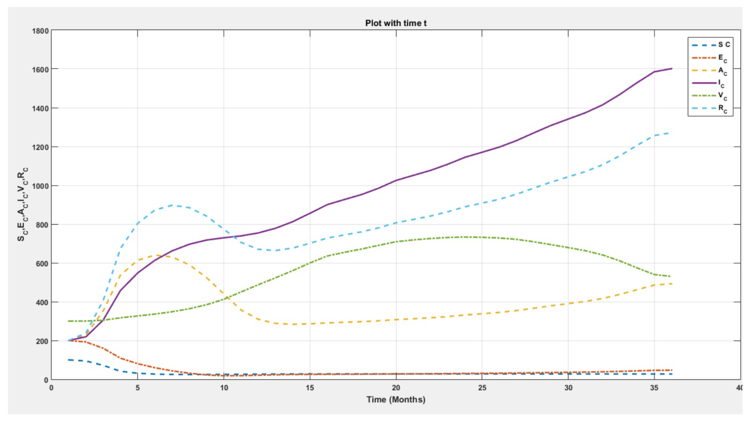
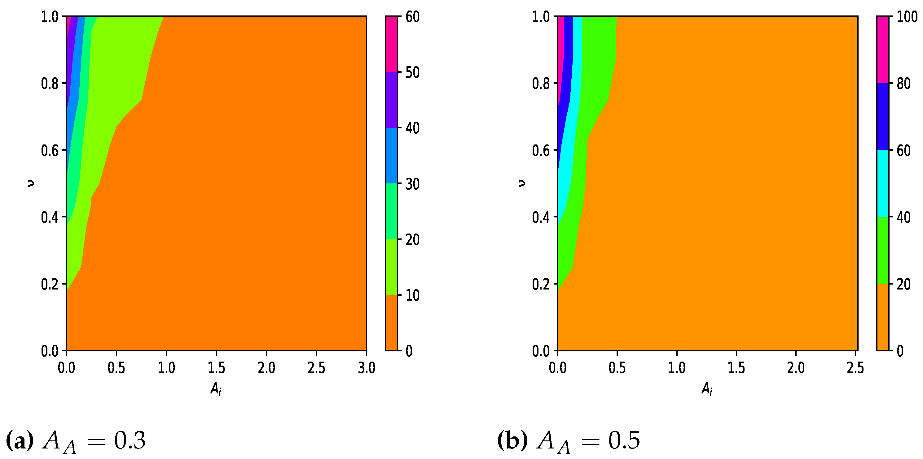
Dynamics of the system are depicted in Figure 1. It shows the steady state behaviour of all the class of populations over the period of time. The contour plots in Figure 2 of reproduction number show that $R_C$ lies between 0 and 20, as the maximum region of the graph is under that shade. Relationship of $R_C$ is depicted in Figure 3 for different values of p. In order to study the effect of the efficacy of vaccine ($\nu$) and the percentage of population being vaccinated on the spread of the COVID-19 epidemic/pandemic, a regular network with size $N={10}^6$ was generated by using the Runge–Kutta method. The effect of efficacy of the vaccination developed for pandemic is simulated in this work. The effect of vaccinated population is also simulated in this study. Overall, the process of spreading the pandemic is simulated in the paper. The impact of vaccination in the spread of the pandemic is shown and demonstrated through simulation with various percentages of efficacy of vaccine and percentage of population vaccinated in a closed region. Initially, the parameters are set as $A_a=0.5$, $A_I=0.25$, $\nu =0$, and ${\lambda }_2=0$.

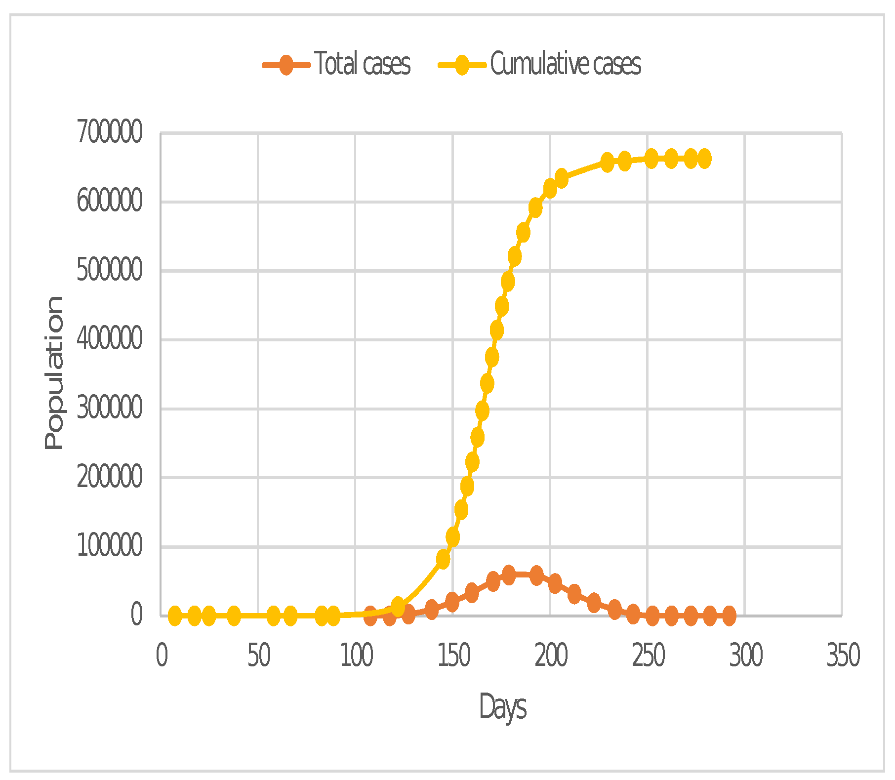
Case I. The transmission rate is ($A_a$) = 0.5, the rate of infected people is ($A_I$) = 0.25, the efficacy of vaccine is ($\nu$) = 0, and the percentage of initially vaccinated population is ${\lambda }_2=0$.

In this case, when there is initially no vaccinated population, this could be considered as the case when the vaccination is not being used for countering any pandemic/COVID-19. As shown in Figure 4, epidemics with large $A_a$ reach their peak quickly, with the total number of cases reaching a maximum of 640,000. Figure 4 shows that the total number of cases reached a maximum of 80,000. (approx.). The pandemic starts to rise rapidly after 100 days.

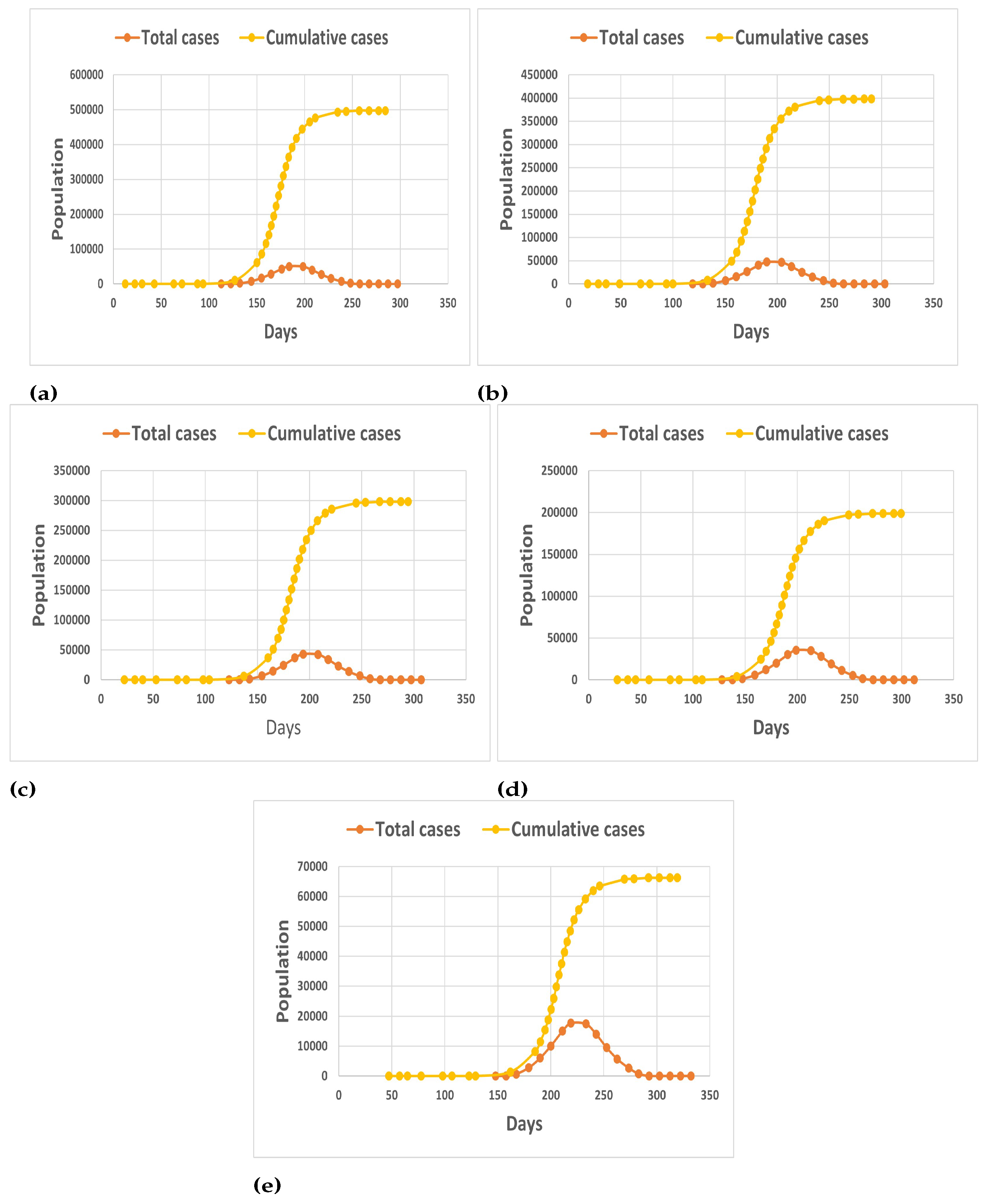
Case II. The transmission rate is ($A_a$) = 0.5, the rate of infected people is ($A_I$) = 0.25, the efficacy of vaccine is ($\nu$) = 0.6, and the percentage of initially vaccinated population is ${\lambda }_2=0$.

This represents the case, when 0 percent of the population is initially vaccinated and the efficacy of the vaccination considered to be 60 percent. It is observed from Figure 5a that there is a slight delay of approximately 5 days in the rise of pandemic, there is a reduction of approximately 25 percent in the cumulative number of cases, and reduction of 15 percent in the total number of current cases.

Case III. The transmission rate is ($A_a$) = 0.5, the rate of infected people is ($A_I$) = 0.25, the efficacy of vaccine is ($\nu$) = 0.6, and the percentage of initially vaccinated population is ${\lambda }_2=0.30$.

In this case, the population that is initially vaccinated is considered to be about 30 percent of the total population and the efficacy of the vaccination used is 60 percent. Figure 5b shows that, compared to Figure 5a of case two, the delay in the onset of the pandemic has increased to 11 days from 5 days. In addition, compared to case one, when the vaccination is not used, the number of cumulative cases is reduced by 40 percent and the total number of cases is reduced by 20 percent.

Case IV. The transmission rate is ($A_a$) = 0.5, the rate of infected people is ($A_I$) = 0.25, the efficacy of vaccine is ($\nu$) = 0.6, and the percentage of initially vaccinated population is ${\lambda }_2=0.50$.

In this case, when the initially vaccinated population has reached around 50 percent of the total population, it means that 50 percent of the population has been vaccinated before any pandemic/ensuing wave of COVID-19 exists in the closed state/territory. In this case, it is observed through Figure 5c that there is a delay of about 15 days in the rapid rise of pandemic cases as compared to Case I, where 0 percent of the population is vaccinated. Additionally, compared to Case I, where the maximum cumulative cases reached around 640,000 and the total number of cases reached a maximum peak of around 50,000 cases on the 200th day of the pandemic, the maximum cumulative cases reached around 300,000 cases. This clearly indicates that if even half of the population is fully vaccinated before the start of any upcoming pandemic wave, there may be a significant reduction of around or greater than 50 percent of cases, compared to when there is no vaccination.

Case V. The transmission rate is ($A_a$) = 0.5, the rate of infected people is ($A_I$) = 0.25, the efficacy of vaccine is ($\nu$) = 0.6, and the percentage of initially vaccinated population is ${\lambda }_2=0.80$.

This is the case when the initially vaccinated population before the pandemic is approximately 80 percent of the total population of the closed state/area. In comparison to Case I, there is a reduction of about 70 percent in cumulative cases and around 40 percent of total cases, as shown in Figure 5d. It is also observed that, in comparison to Case I, the rapid rise of the pandemic/COVID-19 is approximately shifted by 20 days.

Case VI. The transmission rate is ($A_a$) = 0.5, the rate of infected people is ($A_I$) = 0.25, the efficacy of vaccine is ($\nu$) = 0.6, and the percentage of initially vaccinated population is ${\lambda }_2=1$.

Now, we consider an ideal case when the complete population of the closed state is vaccinated before the uprising of the further wave of pandemic, and the efficacy of the vaccination is 60 percent. It could be seen from Figure 5e that there is a huge reduction in the number of cumulative and total infected cases as compared to Case I. It can be seen that cumulative cases have decreased by around 90 percent, demonstrating the importance of vaccination in the eradication of certain diseases.

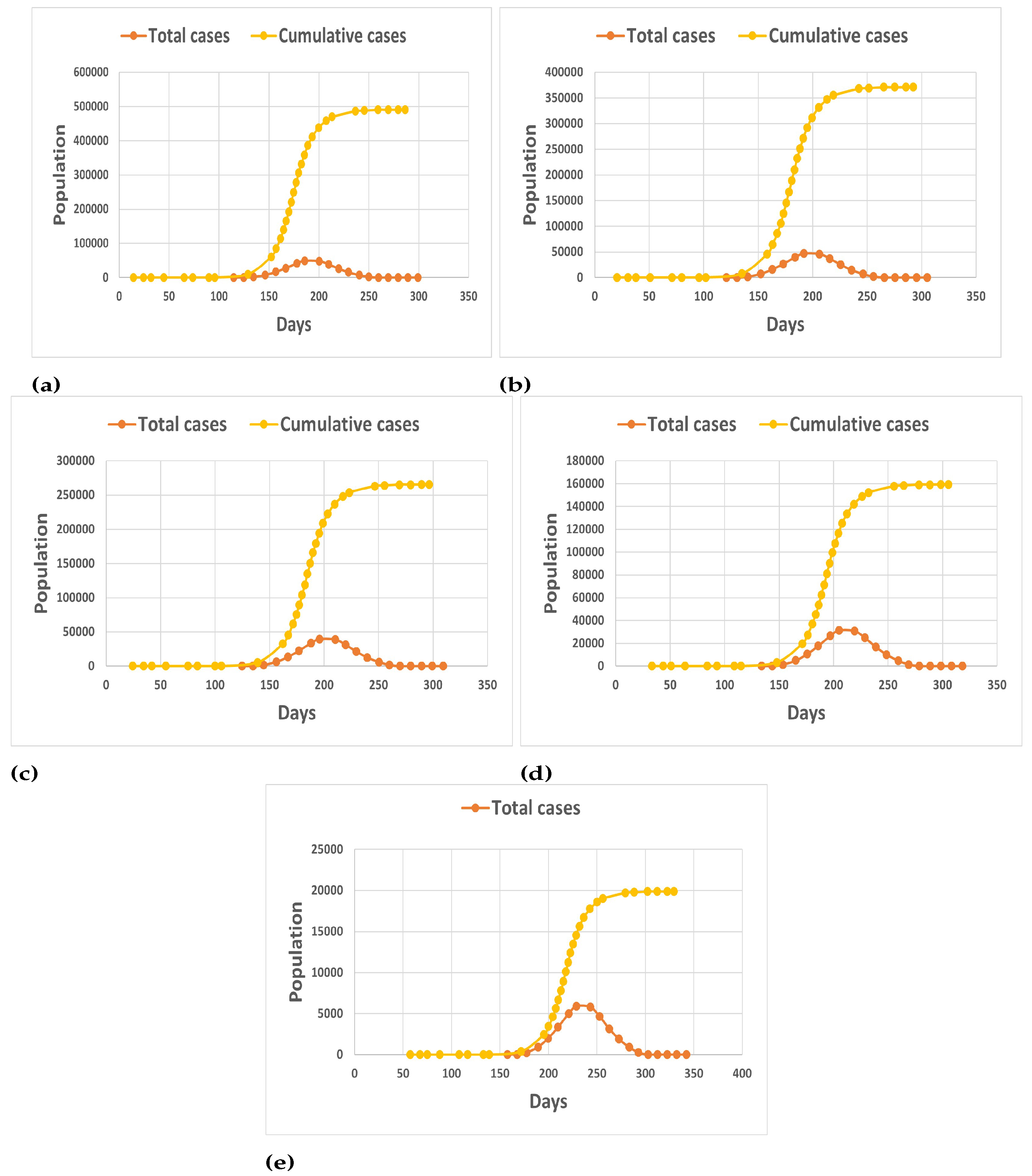
Case VII. The transmission rate is ($A_a$) = 0.5, the rate of infected people is ($A_I$) = 0.25, the efficacy of vaccine is ($\nu$) = 0.7, and the percentage of initially vaccinated population is ${\lambda }_2=0$.

In a new scenario, a case is being considered in which vaccine effectiveness has improved from 60 percent to 70 percent and the population that was initially vaccinated is zero. Figure 6a shows that there is a small variation from Case II, when the efficacy of vaccine was 60 percent. The reduction in the cumulative cases, as compared to Case I, is around 26 percent, the total cases is around 18 percent, and there is a delay of 7 days in the fast rising of the pandemic wave.

Case VIII. The transmission rate is ($A_a$) = 0.5, the rate of infected people is ($A_I$) = 0.25, the efficacy of vaccine is ($\nu$) = 0.7, and the percentage of initially vaccinated population is ${\lambda }_2=0.3$.

In this case, the effect of the previously vaccinated population and the vaccine’s efficacy have been clearly visible and depicted in Figure 6b. Since the pandemic’s initial rapid rise is shifted 13 days ahead, there is a reduction of around 44 percent in the number of cumulative cases and 21 percent in total cases when compared to Case I. In comparison to Case III, where the initial vaccination population is around 30 percent and vaccination efficacy is 60 percent, it is clear that a modest increase of vaccine effectiveness of about 10 percent (from 60 percent to 70 percent) results in a (cumulative) case reduction of approximately 25,000. It shows that increasing vaccine effectiveness while also increasing the number of people who have been vaccinated has a positive impact on epidemic control.

Case IX. The transmission rate is ($A_a$) = 0.5, the rate of infected people is ($A_I$) = 0.25, the efficacy of vaccine is ($\nu$) = 0.7, and the percentage of initially vaccinated population is ${\lambda }_2=0.5$.

Figure 6c shows that, when the initially vaccinated population is covered up to the total population of the closed state, the cumulative cases are reduced by around 60 percent, as compared to around 55 percent in Case IV. In addition, compared to Case IV, the pandemic rise is delayed by two days, demonstrating the importance of vaccine efficacy in pandemic coverage.

Case X. The transmission rate is ($A_a$) = 0.5, the rate of infected people is ($A_I$) = 0.25, the efficacy of vaccine is ($\nu$) = 0.7, and the percentage of initially vaccinated population is ${\lambda }_2=0.8$.

In comparison to Case I, a very good result is obtained, indicating the significant effect of vaccination and the importance of vaccination during pandemics for human survival. Figure 6d shows a 76 percent reduction in cumulative cases and a 26-day delay in the rapid spread of the pandemic when compared to Case I. In comparison to Case V, when the vaccine’s efficacy was 60 percent and all other factors remained the same, the vaccine’s efficacy has improved dramatically, resulting in a massive reduction of around 40,000 cases.

Case XI. The transmission rate is ($A_a$) = 0.5, the rate of infected people is ($A_I$) = 0.25, the efficacy of vaccine is ($\nu$) = 0.7, and the percentage of initially vaccinated population is ${\lambda }_2=1$.

Figure 6e shows that, if 100 percent of the population is vaccinated, there is a 97 percent reduction in cumulative cases compared to Case I. The maximum cumulative case reaches 20,000. In comparison to Case I, there is a 50-day delay in the rapid spread of pandemic. It is evident that having a highly vaccinated population can become a major factor in controlling and declining a pandemic wave.

Case XII. The transmission rate is ($A_a$) = 0.5, the rate of infected people is ($A_I$) = 0.25, the efficacy of vaccine is ($\nu$) = 0.8, and the percentage of initially vaccinated population ${\lambda }_2=0.5$.

In this case, it is considered that 50 percent of total population is being vaccinated and the efficacy of vaccination has reached up to 80 percent. We can conclude, from Figure 7a, that a reduction of around 65 percent in cumulative cases is obtained as compared to Case I. In addition, in comparison to Case IV, where vaccine efficacy is 60 percent while all other factors remain constant, cumulative cases show a reduction of around 10 percent, indicating the effect of vaccine efficacy on pandemic control.

Case XIII. The transmission rate is ($A_a$) = 0.5, the rate of infected people is ($A_I$) = 0.25, the efficacy of vaccine is ($\nu$) = 0.8, and the percentage of initially vaccinated population is ${\lambda }_2=1$.

Figure 7b shows that, in this ideal special case, where the entire population is vaccinated and the vaccine efficacy is around 80 percent, the maximum pandemic (cumulative, Case I) is reduced by 99 percent and the pandemic rise is delayed by more than 2 months.The maximum number of cumulative cases has fallen below 7000, indicating the critical importance of vaccination for human survival, as compared to Case VI and Case XI, where the efficacy of vaccine is 60 and 70 percent, respectively. It can be seen that the maximum cumulative cases for both cases are around 70,000 and 20,000, respectively. With 100 percent of population vaccinated, the importance of quality of vaccination also matters.

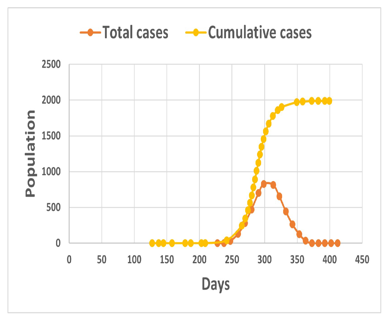
Case XIV. The transmission rate is ($A_a$) = 0.5, the rate of infected people is ($A_I$) = 0.25, the efficacy of vaccine is ($\nu$) = 0.9, and the percentage of initially vaccinated population is ${\lambda }_2=1$.

In this case, when 100 percent of the total closed population is vaccinated with a vaccination with 90 percent efficacy, Figure 8 clearly shows that the maximum number of cumulative cases has reached 2000 cases. A delay of around 4 months in the rise of pandemic wave is obtained, clearly indicating that a vaccine with very good efficacy and percentage of vaccinated population are both important to curb the fatal pandemic waves and save thousands of lives.

4. Conclusions and Future Work

System dynamics is demonstrated in Figure 1, which represents the steady state behaviour of different cases of population with respect to time. Represented contour plot in Figure 2 shows that reproduction number ($R_c$) lies between 0 and 20. The COVID-19 pandemic is spreading very rapidly. As the number of cases increases, vaccination has become an important tool in preventing disease spread. The experiment in this study is carried out by varying the values of two major factors: vaccination’s effectiveness in controlling epidemic spread and analysing its impact, as well as the percentage of the population vaccinated, in a closed stage.

Both cases where the initial population was not vaccinated and cases where there is an increase in vaccination are considered, and it has been discovered that the cumulative cases decrease with an increase in vaccination, highlighting the importance of vaccine efficacy. When vaccination is kept consistent and a large percentage of the initial population is vaccinated, cumulative cases are reduced and epidemics are delayed. Furthermore, when both vaccine efficacy and the percentage of the total vaccinated population are considered, the pandemic wave is greatly reduced. If the population vaccinated is above 70 percent and efficacy of vaccine is considered between 60–90 percent, then the total vaccinated population percentage factor overpowers the efficacy of vaccine. When vaccination rates reach 80 percent and the initial total vaccinated population exceeds 50 percent, vaccine efficacy becomes a more influential factor. It can be inferred that both factors are important to curb the epidemic, i.e., a vaccine with good efficacy and the total initial vaccinated population. As a result, multiple types of vaccines with varying efficacy could be used to vaccinate the entire population at first and a little difference between the efficacy of vaccines is not a significant factor. In contrast, vaccination of a large population is much more important in preventing the expected pandemic waves. In the future, a mathematical delay parameter can be added to the model and the results could be validated.