
Does Climate Play Any Role in COVID-19 Spreading?—An Australian Perspective


Abstract
:1. Introduction
2. Methodology
2.1. Data Collection
2.2. Statistical Analysis
3. Results
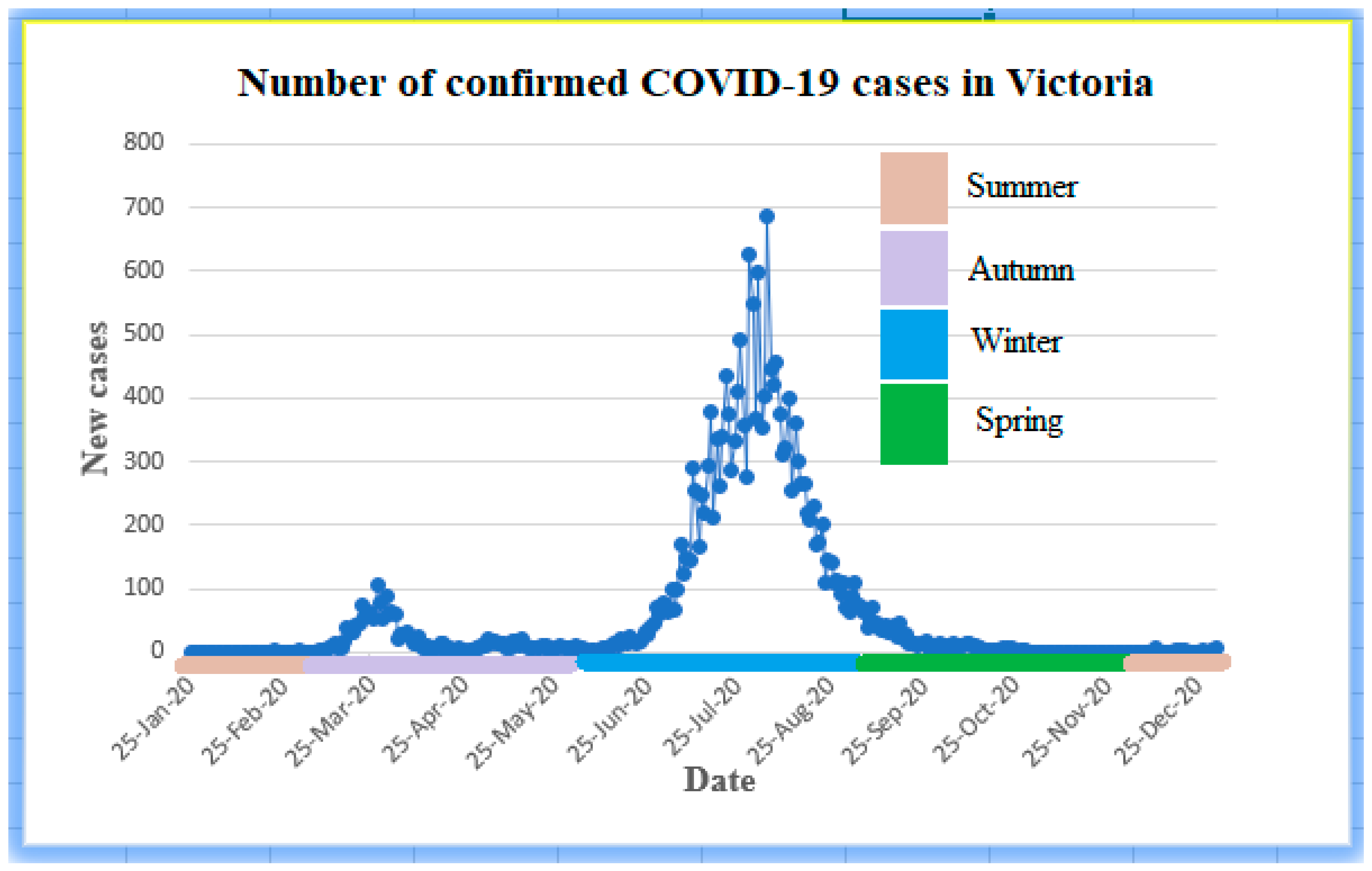
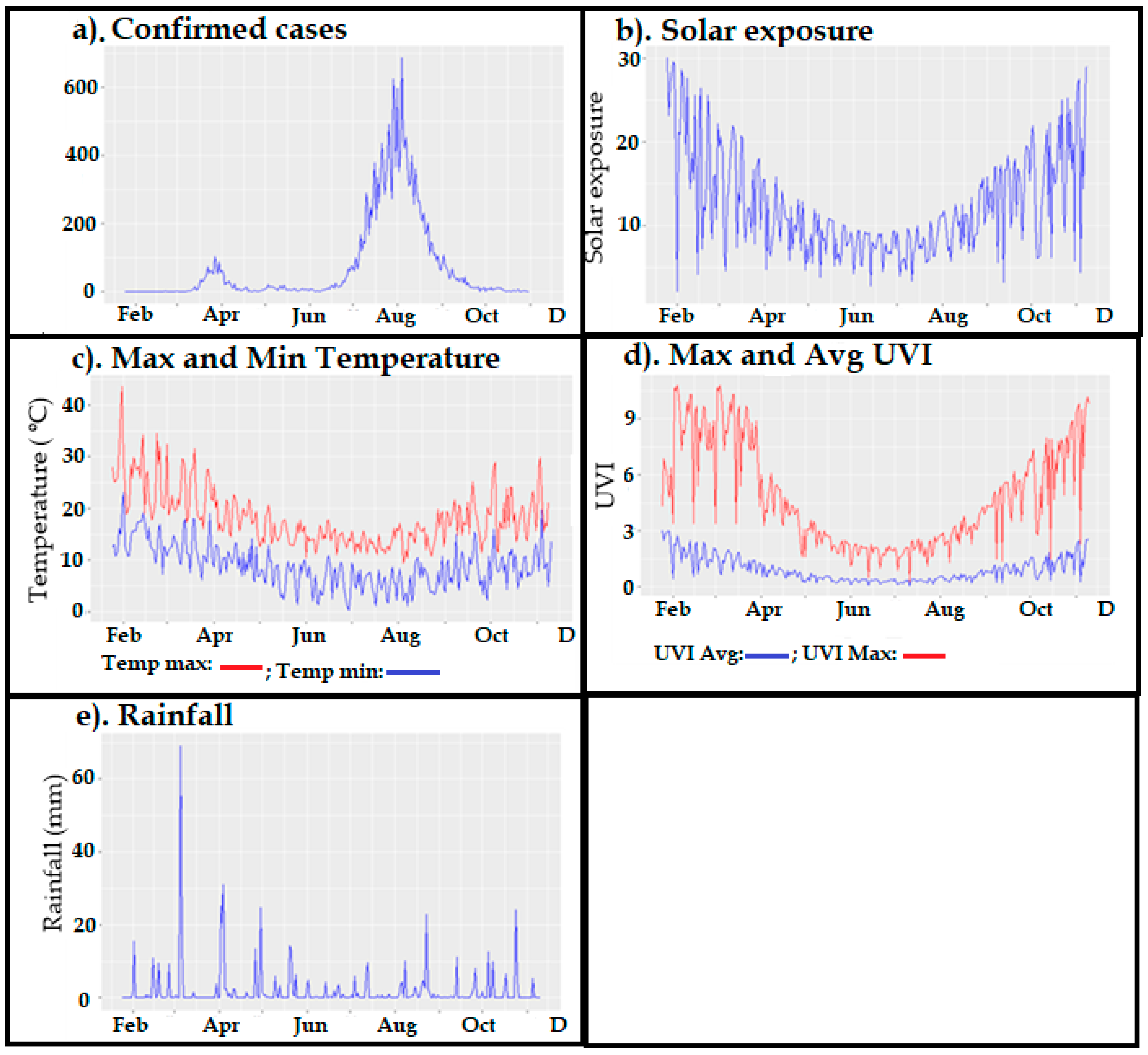
3.1. Descriptive Analyses
3.2. Correlation Analysis of Original and Stationary Times Series
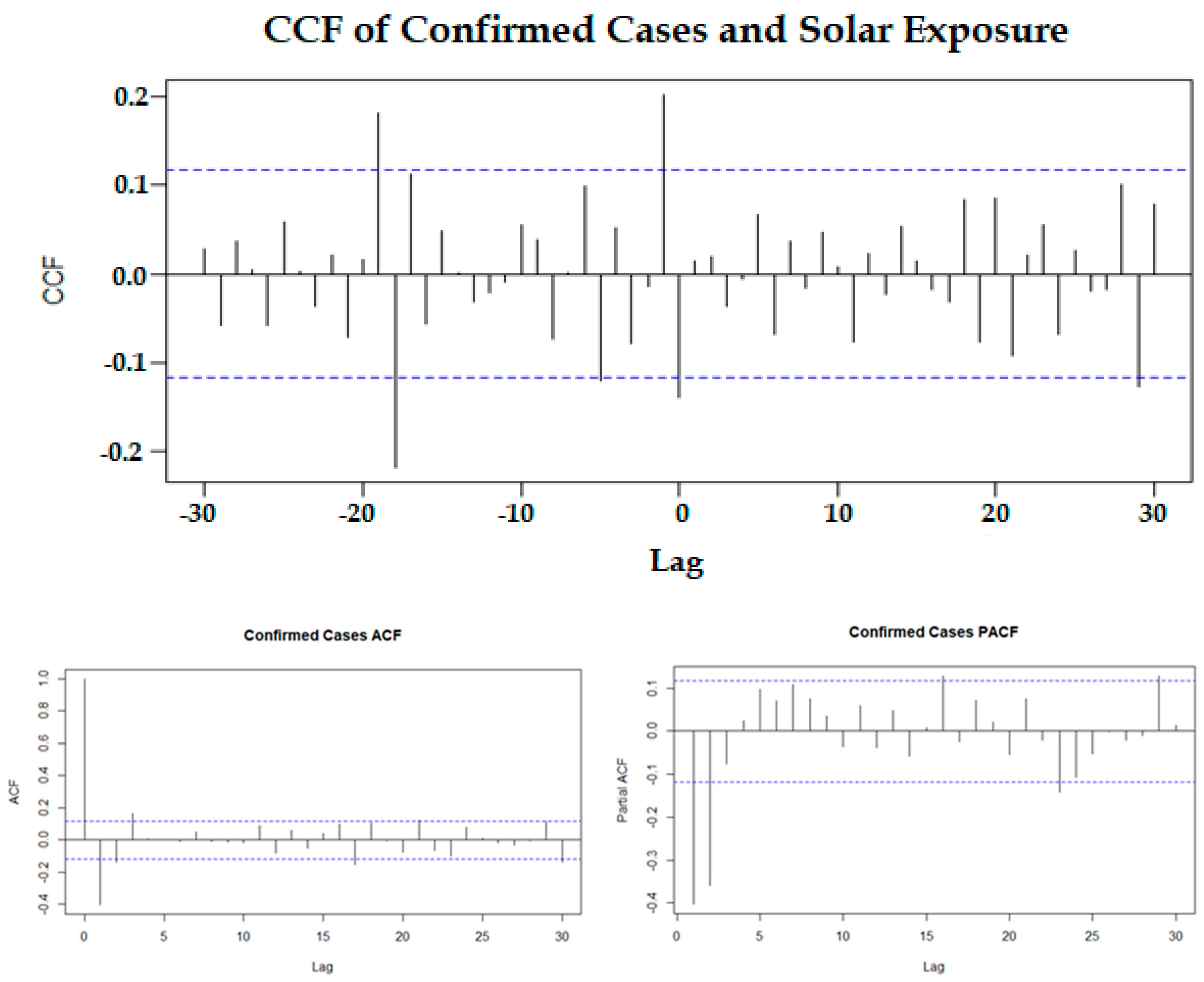
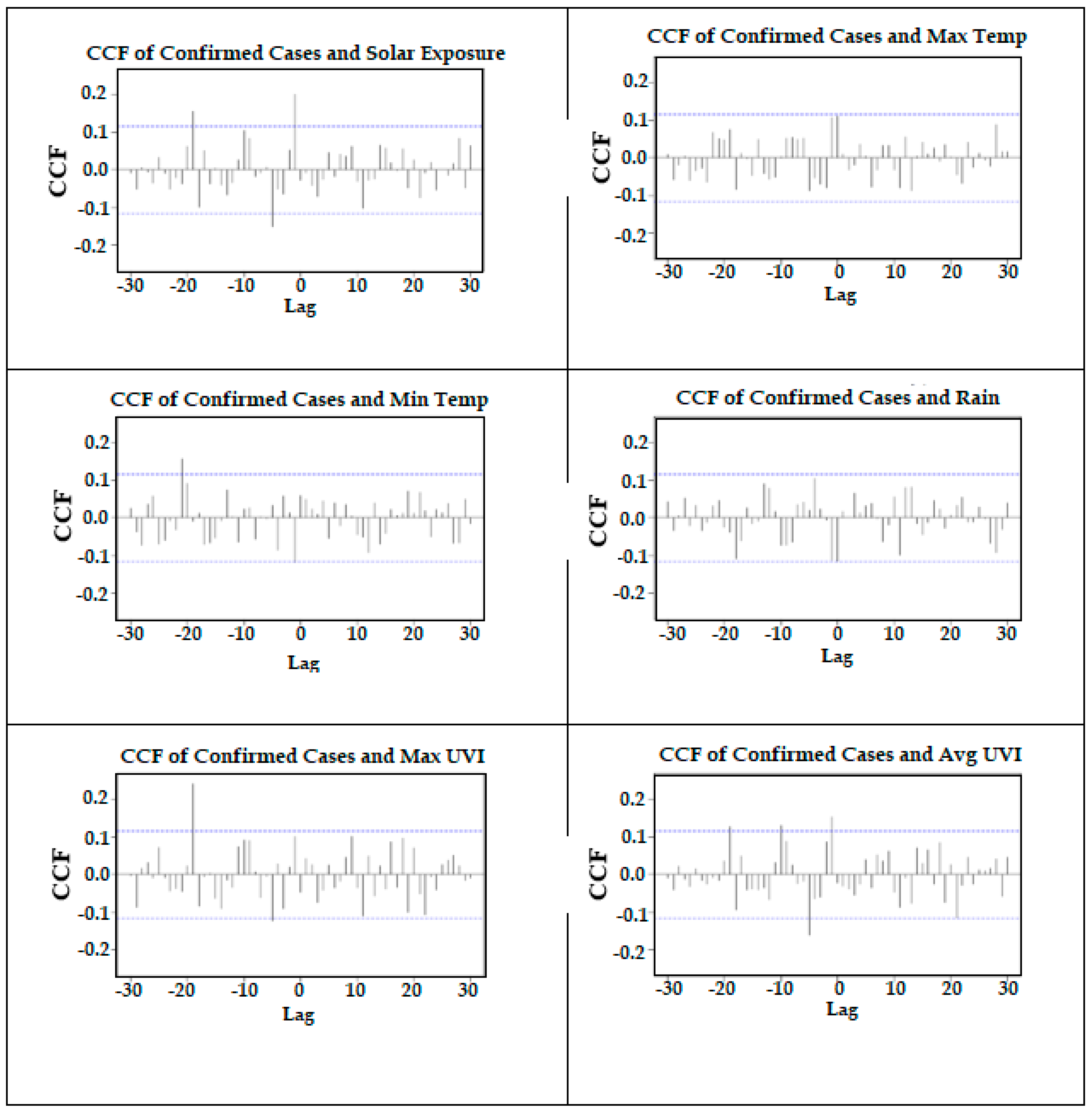
3.3. Correlation Analysis after Pre-Whitening the Time Series
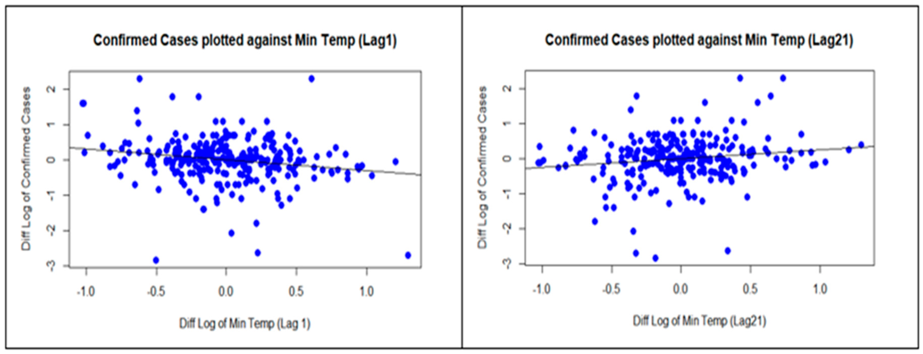
3.4. Regression on Significant Correlations
4. Discussion
5. Conclusions
Author Contributions
Funding
Institutional Review Board Statement
Informed Consent Statement
Acknowledgments
Conflicts of Interest
References
- Health Australia. Department of Health, Australian Government. Available online: www.health.gov.au (accessed on 12 January 2021).
- Roussel, M.; Pontier, D.; Cohen, J.-M.; Lina, B.; Fouchet, D. Quantifying the role of weather on seasonal influenza. BMC Public Health 2016, 16, 441. [Google Scholar] [CrossRef] [Green Version]
- Ianevski, A.; Zusinaite, E.; Shtaida, N.; Kallio-Kokko, H.; Valkonen, M.; Kantele, A.; Telling, K.; Lutsar, I.; Letjuka, P.; Metelitsa, N.; et al. Low temperature and low UV indexes correlated with peaks of influenza virus activity in Northern Europe during 2010–2018. Viruses 2019, 11, 207. [Google Scholar] [CrossRef] [PubMed] [Green Version]
- Quilodran, C.S.; Currat, M.; Montoya-Burgos, J.I. Climatic factors influence COVID-19 outbreak as revealed by worldwide mortality. MedRxiv 2020. [Google Scholar] [CrossRef] [Green Version]
- Dbouk, T.; Drikakis, D. Weather impact on airborne coronavirus survival. Phys. Fluids 2020, 32, 093312. [Google Scholar] [CrossRef] [PubMed]
- Ramírez, I.J.; Lee, J. Ecosyndemic vulnerability: Implications for El Niño-sensitive countries in Latin America. Int. J. Disaster Risk Sci. 2021, 12, 147–156. [Google Scholar] [CrossRef]
- Moozhipurath, R.K. Role of Weather Factors in COVID-19 Death Growth Rates in Tropical Climate: A Data-Driven Study Focused on Brazil. MedRXiv 2020. [Google Scholar] [CrossRef]
- Takagi, H.; Kuno, T.; Yokoyama, Y.; Ueyama, H.; Matsushiro, T.; Hari, Y.; Ando, T. The higher temperature and ultraviolet, the lower COVID-19 prevalence–meta-regression of data from large US cities. Am. J. Infect. Control 2020, 48, 1281–1285. [Google Scholar] [CrossRef]
- Rhodes, J.; Dunstan, F.; Laird, E.; Subramanian, S.; Kenny, R.A. COVID-19 mortality increases with northerly latitude after adjustment for age suggesting a link with ultraviolet and vitamin D. BMJ Nutr. Prev. Health 2020, 3, 118–120. [Google Scholar] [CrossRef]
- Islam, N.; Bukhari, Q.; Jameel, Y.; Shabnam, S.; Erzurumluoglu, A.; Siddique, M.A.; Massaro, J.M.; D’Agostino, R.B. COVID-19 and climatic factors: A global analysis. Environ. Res. 2021, 193, 110355. [Google Scholar] [CrossRef]
- Yao, Y.; Pan, J.; Liu, Z.; Meng, X.; Wang, W.; Kan, H.; Wang, W. No association of COVID-19 transmission with temperature or UV radiation in Chinese cities. Eur. Respir. J. 2020, 55, 2000517. [Google Scholar] [CrossRef] [Green Version]
- Blumthaler, M. UV monitoring for public health. Int. J. Environ. Res. Public Health 2018, 15, 1723. [Google Scholar] [CrossRef] [Green Version]
- Casini, B.; Tuvo, B.; Cristina, M.L.; Spagnolo, A.M.; Totaro, M.; Baggiani, A.; Privitera, G.P. Evaluation of an ultraviolet C (UVC) light-emitting device for disinfection of high touch surfaces in hospital critical areas. Int. J. Environ. Res. Public Health 2019, 16, 3572. [Google Scholar] [CrossRef] [PubMed] [Green Version]
- Hanel, A.; Carlberg, C. Skin colour and vitamin D: An update. Exp. Dermatol. 2020, 29, 864–875. [Google Scholar] [CrossRef] [PubMed]
- Hart, P.H.; Gorman, S.; Finlay-Jones, J.J. Modulation of the immune system by UV radiation: More than just the effects of vitamin D? Nat. Rev. Immunol. 2011, 11, 584–596. [Google Scholar] [CrossRef] [PubMed]
- Han, Y.; Lam, J.C.; Li, V.O.; Guo, P.; Zhang, Q.; Wang, A.; Downey, J. The effects of outdoor air pollution concentrations and lockdowns on COVID-19 infections in Wuhan and other provincial capitals in China. Preprints 2020. [Google Scholar] [CrossRef]
- Arunachalam, P.S.; Wimmers, F.; Mok, C.K.P.; Perera, R.A.P.M.; Scott, M.; Hagan, T.; Sigal, N.; Feng, Y.; Bristow, L.; Tsang, O.T.-Y.; et al. Systems biological assessment of immunity to mild versus severe COVID-19 infection in humans. Science 2020, 369, 1210–1220. [Google Scholar] [CrossRef]
- Fang, X.; Li, S.; Yu, H.; Wang, P.; Zhang, Y.; Chen, Z.; Li, Y.; Cheng, L.; Li, W.; Jia, H.; et al. Epidemiological, comorbidity factors with severity and prognosis of COVID-19: A systematic review and meta-analysis. Aging 2020, 12, 12493–12503. [Google Scholar] [CrossRef]
- WHO. Rational Use of Personal Protective Equipment for COVID-19 and Considerations during Severe Shortages: Interim Guidance, 23 December 2020 (No. WHO/2019-nCoV/IPC_PPE_use/2020.4); World Health Organization: Geneva, Switzerland, 2020. [Google Scholar]
- Gupta, S.; Raghuwanshi, G.S.; Chanda, A. Effect of weather on COVID-19 spread in the US: A prediction model for India in 2020. Sci. Total Environ. 2020, 728, 138860. [Google Scholar] [CrossRef]
- Şahin, M. Impact of weather on COVID-19 pandemic in Turkey. Sci. Total Environ. 2020, 728, 138810. [Google Scholar] [CrossRef]
- Tosepu, R.; Gunawan, J.; Effendy, D.S.; Lestari, H.; Bahar, H.; Asfian, P. Correlation between weather and COVID-19 pandemic in Jakarta, Indonesia. Sci. Total Environ. 2020, 725, 138436. [Google Scholar] [CrossRef] [PubMed]
- Department of Health. State Government of Victoria, Australia. Available online: www.vic.gov.au (accessed on 26 June 2021).
- BOM. Bureau of Meteorology, Australian Government. Available online: http://www.bom.gov.au/climate/data/?ref=ftr (accessed on 20 December 2020).
- Chatfield, C.; Xing, H. The Analysis of Time Series: An Introduction with R, 7th ed.; Chapman & Hall, CRC Press: Boca Raton, FL, USA, 2019. [Google Scholar]
- Douglas, E.; Vogel, R.; Kroll, C. Trends in floods and low flows in the United States: Impact of spatial correlation. J. Hydrol. 2000, 240, 90–105. [Google Scholar] [CrossRef]
- Briet, O.J.; Vounatsou, P.; Gunawardena, D.M.; Galappaththy, G.N.; Amerasinghe, P.H. Temporal correlation between malaria and rainfall in Sri Lanka. Malar. J. 2008, 7, 77. [Google Scholar] [CrossRef] [PubMed] [Green Version]
- Probst, W.N.; Stelzenmüller, V.; Fock, H.O. Using cross-correlations to assess the relationship between time-lagged pressure and state indicators: An exemplary analysis of North Sea fish population indicators. ICES J. Mar. Sci. 2012, 69, 670–681. [Google Scholar] [CrossRef] [Green Version]
- Dean, R.T.; Dunsmuir, W.T.M. Dangers and uses of Cross-Correlation in analyzing time series in perception, performance, movement, and neuroscience: The importance of constructing transfer function autoregressive models. Behav. Res. Methods 2015, 48, 783–802. [Google Scholar] [CrossRef] [Green Version]
- Earnest, A.; Chen, M.I.; Ng, D.; Sin, L.Y. Using autoregressive integrated moving average (ARIMA) models to predict and monitor the number of beds occupied during a SARS outbreak in a tertiary hospital in Singapore. BMC Health Serv. Res. 2005, 5, 36. [Google Scholar] [CrossRef] [PubMed] [Green Version]
- Chen, T.; Leng, K.; Lu, Y.; Wen, L.; Qi, Y.; Gao, W.; Chen, H.; Bai, L.; An, X.; Sun, B.; et al. Epidemiological features and time-series analysis of influenza incidence in urban and rural areas of Shenyang, China, 2010–2018. Epidem. Infect. 2020, 148, e29. [Google Scholar] [CrossRef] [PubMed] [Green Version]
- Lee, D.; Kim, Y.; Koh, Y.; Song, K.; Chang, I. Forecasting COVID-19 confirmed cases using empirical data analysis in Korea. Healthcare 2021, 9, 254. [Google Scholar] [CrossRef]
- Akaike, H. Information theory and an extension of the maximum likelihood principle. In Second International Symposium on Information Theory; Kotz, S., Johnson, N.L., Eds.; Academia Kiado: Budapest, Hungary, 1973; pp. 267–281. [Google Scholar]
- Casanova, L.M.; Jeon, S.; Rutala, W.A.; Weber, D.J.; Sobsey, M.D. Effects of air temperature and relative humidity on coronavirus survival on surfaces. Appl. Environ. Microbiol. 2010, 76, 2712–2717. [Google Scholar] [CrossRef] [Green Version]
- Chan, K.H.; Peiris, J.S.M.; Lam, S.Y.; Poon, L.L.M.; Yuen, K.-Y.; Seto, W.H. The effects of temperature and relative humidity on the viability of the SARS coronavirus. Adv. Virol. 2011, 2011, 734690. [Google Scholar] [CrossRef]
- Rehman, A.; Ashraf, F.; Javed, Z.; Hussain, M.; Farooq, T.H.; Shakoor, A.; Shahzad, S.M. The nexus between meteorological parameters and COVID-19 pandemic: Case of Islamabad, Pakistan. Environ. Sustain. 2020, 1–5. [Google Scholar] [CrossRef]
- Arumugam, M.; Menon, B.; Narayan, S.K. Ambient temperature and COVID-19 incidence rates: An opportunity for intervention? 2020. Available online: https://ojs.wpro.who.int/ojs/public/journals/1/covid19/wpsar.2020.11.5.012Arumugam.pdf (accessed on 20 March 2021).
- Caspi, G.; Shalit, U.; Kristensen, S.L.; Aronson, D.; Caspi, L.; Rossenberg, O.; Caspi, O. Climate effect on COVID-19 spread rate: An online surveillance tool. medRxiv 2020. [Google Scholar] [CrossRef] [Green Version]
- Wang, J.; Tang, K.; Feng, K.; Lv, W. High temperature and high humidity reduce the transmission of COVID-19. arXiv preprint 2020, arXiv:2003.05003v5. [Google Scholar] [CrossRef] [Green Version]
- Kubota, Y.; Shiono, T.; Kusumoto, B.; Fujinuma, J. Multiple drivers of the COVID-19 spread: The roles of climate, international mobility, and region-specific conditions. PLoS ONE 2020, 15, e0239385. [Google Scholar] [CrossRef] [PubMed]
- Asyary, A.; Veruswati, M. Sunlight exposure increased Covid-19 recovery rates: A study in the central pandemic area of Indonesia. Sci. Total. Environ. 2020, 729, 139016. [Google Scholar] [CrossRef] [PubMed]
- Cannell, J.J.; Vieth, R.; Umhau, J.C.; Holick, M.F.; Grant, W.B.; Madronich, S.; Garland, C.F.; Giovannucci, E. Epidemic influenza and vitamin D. Epidemiol. Infect. 2006, 134, 1129–1140. [Google Scholar] [CrossRef] [PubMed]
- Bergman, P. The link between vitamin D and COVID-19: Distinguishing facts from fiction. J. Intern. Med. 2021, 289, 131–133. [Google Scholar] [CrossRef]
- Grant, W.B.; Lahore, H.; McDonnell, S.L.; Baggerly, C.A.; French, C.B.; Aliano, J.L.; Bhattoa, H.P. Evidence that vitamin D supplementation could reduce risk of influenza and COVID-19 infections and deaths. Nutrients 2020, 12, 988. [Google Scholar] [CrossRef] [PubMed] [Green Version]
- Maghbooli, Z.; Sahraian, M.A.; Ebrahimi, M.; Pazoki, M.; Kafan, S.; Tabriz, H.M.; Hadadi, A.; Montazeri, M.; Nasiri, M.; Shirvani, A.; et al. Vitamin D sufficiency, a serum 25-hydroxyvitamin D at least 30 ng/mL reduced risk for adverse clinical outcomes in patients with COVID-19 infection. PLoS ONE 2020, 15, e0239799. [Google Scholar] [CrossRef]
- Cohen, J. Sick time. Science 2020, 367, 1294–1297. [Google Scholar] [CrossRef] [Green Version]
- Rosario, D.K.A.; Mutz, Y.S.; Bernardes, P.C.; Conte-Junior, C.A. Relationship between COVID-19 and weather: Case study in a tropical country. Int. J. Hyg. Environ. Health 2020, 229, 113587. [Google Scholar] [CrossRef]
- Moriyama, M.; Hugentobler, W.J.; Iwasaki, A. Seasonality of respiratory viral infections. Annu. Rev. Virol. 2020, 7, 83–101. [Google Scholar] [CrossRef] [PubMed]
- Abraham, J.; Dowling, K.; Florentine, S. Can Optimum Solar Radiation Exposure or Supplemented Vitamin D Intake Reduce the Severity of COVID-19 Symptoms? Int. J. Environ. Res. Public Health 2021, 18, 740. [Google Scholar] [CrossRef] [PubMed]
- Bilezikian, J.P.; Bikle, D.; Hewison, M.; Lazaretti-Castro, M.; Formenti, A.M.; Gupta, A.; Madhavan, M.V.; Nair, N.; Babalyan, V.; Hutchings, N.; et al. Mechanisms in endocrinology: Vitamin D and COVID-19. Eur. J. Endocrinol. 2020, 183, R133–R147. [Google Scholar] [CrossRef]
- Ratnesar-Shumate, S.; Williams, G.; Green, B.; Krause, M.; Holland, B.; Wood, S.; Bohannon, J.; Boydston, J.; Freeburger, D.; Hooper, I.; et al. Simulated sunlight rapidly inactivates SARS-CoV-2 on surfaces. J. Infect. Dis. 2020, 222, 214–222. [Google Scholar] [CrossRef] [PubMed]


| Variables | Mean | SD | Min | Max |
|---|---|---|---|---|
| Confirmed cases | 72.39 | 128.25 | 0 | 687 |
| Solar exposure (MJ/m2) | 12.16 | 5.88 | 2.1 | 30.1 |
| Maximum UVI | 4.64 | 2.71 | 0.3 | 10.8 |
| Average UVI | 0.89 | 0.64 | 0.40 | 3.03 |
| Maximum Temperature (°C) | 18.16 | 5.46 | 14.3 | 43.6 |
| Minimum Temperature (°C) | 8.75 | 4.12 | 0.2 | 23.0 |
| Rainfall (mm) | 1.91 | 5.96 | 0 | 69 |
| Meteorological Variable | Original Time Series | Stationary Time Series | ||
|---|---|---|---|---|
| Pearson | Spearman | Pearson | Spearman | |
| Solar Exposure (MJ/m2) | −0.265 (<0.001) | −0.349 (<0.001) | −0.139 (0.020) | −0.131 (0.028) |
| Max UVI | −0.374 (<0.001) | −0.472 (<0.001) | −0.131 (0.029) | −0.172 (0.004) |
| Average UVI | −0.357 (<0.001) | −0.506 (<0.001) | −0.104 (0.082) | −0.082 (0.170) |
| Max Temp (°C) | −0.379 (<0.001) | −0.490 (<0.001) | 0.076 (0.203) | 0.056 (0.355) |
| Min Temp (°C) | −0.388 (<0.001) | −0.464 (<0.001) | 0.112 (0.062) | 0.032 (0.595) |
| Rainfall (mm) | −0.062 (0.299) | −0.010 (0.861) | −0.071 (0.238) | −0.126 (0.035) |
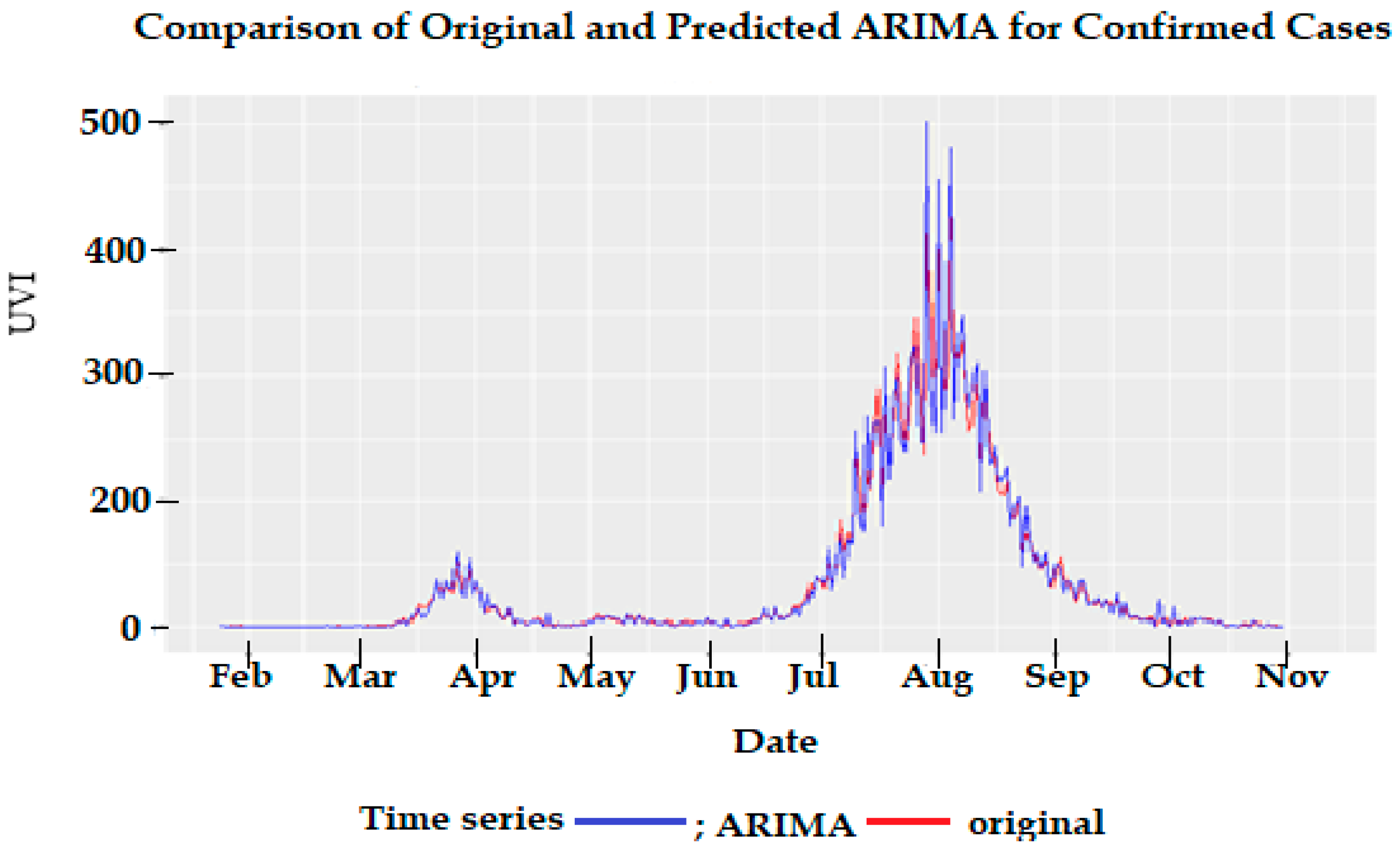
| ar1 | ar2 | ma1 | ma2 | |
|---|---|---|---|---|
| Coefficient | 0.717 | −0.199 | −1.339 | 0.646 |
| SE | 0.159 | 0.089 | 0.144 | 0.094 |
| p-value | <0.001 | 0.024 | <0.001 | <0.001 |
| AIC | 447.49 |
| Meteorological Parameters | Sig. Lags from CCF | Correlation of Sig. Lags | p-Value of Sig. Lags |
|---|---|---|---|
| Solar exposure (MJ/m2) | 1 | 0.205 | <0.001 |
| 5 | −0.155 | 0.010 | |
| 19 | 0.166 | 0.007 | |
| Max UV | 5 | −0.126 | 0.038 |
| 19 | 0.267 | <0.001 | |
| Average UV | 1 | 0.158 | 0.008 |
| 5 | −0.165 | 0.006 | |
| 10 | 0.139 | 0.023 | |
| 19 | 0.141 | 0.023 | |
| Max Temp (°C) | Nil | ||
| Min Temp (°C) | 1 | −0.119 | 0.046 |
| 21 | 0.162 | 0.009 | |
| Rainfall (mm) | Nil |
| Meteorological Parameters | Sig. Lags from Regr | Regr Coeff | 95% CI | p-Value | R-sq |
|---|---|---|---|---|---|
| Solar exposure (MJ/m2) | 1 | 0.320 | 0.138, 0.502 | <0.001 | 10.9% |
| 5 | −0.269 | −0.457, −0.081 | 0.004 | ||
| 19 | 0.313 | 0.133, 0.505 | <0.001 | ||
| Max Temp (°C) | Nil | ||||
| Min Temp(°C) | 1 | −0.303 | −0.493, −0.113 | 0.002 | 6.3% |
| 21 | 0.238 | 0.044, 0.432 | 0.015 | ||
| Rainfall (mm) | Nil | ||||
| Max UV | 5 | −0.258 | −0.512, 0.004 | 0.044 | 10.7% |
| 19 | 0.706 | 0.434, 0.978 | <0.001 | ||
| Average UV | 1 | 0.468 | 0.042, 0.894 | 0.029 | 7.1% |
| 5 | −0.531 | −0.957, −0.105 | 0.013 | ||
| 19 | 0.631 | 0.201, 1.61 | 0.004 |
Publisher’s Note: MDPI stays neutral with regard to jurisdictional claims in published maps and institutional affiliations. |
© 2021 by the authors. Licensee MDPI, Basel, Switzerland. This article is an open access article distributed under the terms and conditions of the Creative Commons Attribution (CC BY) license (https://creativecommons.org/licenses/by/4.0/).
Share and Cite
Abraham, J.; Turville, C.; Dowling, K.; Florentine, S. Does Climate Play Any Role in COVID-19 Spreading?—An Australian Perspective. Int. J. Environ. Res. Public Health 2021, 18, 9086. https://doi.org/10.3390/ijerph18179086
Abraham J, Turville C, Dowling K, Florentine S. Does Climate Play Any Role in COVID-19 Spreading?—An Australian Perspective. International Journal of Environmental Research and Public Health. 2021; 18(17):9086. https://doi.org/10.3390/ijerph18179086
Chicago/Turabian StyleAbraham, Joji, Christopher Turville, Kim Dowling, and Singarayer Florentine. 2021. "Does Climate Play Any Role in COVID-19 Spreading?—An Australian Perspective" International Journal of Environmental Research and Public Health 18, no. 17: 9086. https://doi.org/10.3390/ijerph18179086