Entropy-Based Informational Study of the COVID-19 Series of Data

Abstract

Since the appearance in China of the first cases, the entire world has been deeply affected by the flagellum of the Coronavirus Disease (COVID-19) pandemic. There have been many mathematical approaches trying to characterize the data collected about this serious issue. One of the most important aspects for attacking a problem is knowing what information is really available. We investigate here the information contained in the COVID-19 data of infected and deceased people in all countries, using informational quantifiers such as entropy and statistical complexity. For the evaluation of these quantities, we use the Bandt–Pompe permutation methodology, as well as the wavelet transform, to obtain the corresponding probability distributions from the available series of data. The period analyzed covers from the appearance of the disease up to the massive use of anti-COVID vaccines.

1. Introduction

Regarding the Coronavirus Disease (COVID-19) pandemic, many deterministic and stochastic mathematical methods have been used to model the curves of daily new confirmed cases, deaths, etc, and also to predict future behaviors such as peaks and troughs. However, those methods might present some difficulties [1]. A plausible explanation of this could be the enormous number of variables for modeling a disease in a globalized world, with national and even regional cultural diversities, or maybe the inherent characteristics of the propagation of the SARS-CoV-2 virus, among many other plausible ideas.

Given a time series, there are different ways to quantify the uncertainty associated with it. In connection with the COVID-19 series of data, several stochastic models have been introduced. Correlation functions and associated probability density functions have been computed. Karhunen–Loève expansion KLE is an approach that allows for solving PDEs stochastically and provides high-order moments with relatively little computational effort [2]. In this method, the coefficients are random variables and basis functions employed are determined by the covariance function of the process. In this way, the Karhunen–Loève transform adapts to the process in order to produce the best possible basis for its expansion. In addition, one can mention the probability transformation method [3] and no-probabilistic approaches as the fuzzy set theory [4].

Here, we attack the problem from a different point of view: we look for the information contained in the available data of the COVID-19 pandemic collected all around the world, and our goal is to quantify that information content. For this purpose, we use statistical tools of recognized efficiency in different fields [5]. Our analysis focuses on the period previous to massive vaccination, as this is the lapse with the greatest randomness in the available data.This was the period in which the infection was able to exhibit its intrinsic dynamics of spread, except for the well-known interventions of world governments through their health policies (mainly lockdown).

Entropy is undoubtedly one of the basic concepts of science. Without this concept, the description of reality given by physics would not be possible, nor would many technological advances have taken place. Since Claude Shannon introduced in 1948 the concept of information entropy [6], different measures based on information theory (IT) have occupied an important position in several fields of research [7,8,9,10,11,12,13,14]. More recently, another family of quantifiers known as statistical complexities [15,16] have also contributed in different scenarios, allowing for studying time series regardless of their sources, and to obtain “hidden” a priori information (see, among others, [17,18,19,20,21,22]).

In the present contribution, our proposal is to take advantage of different information-theoretic quantifiers, namely Shannon entropy and statistical complexity, to meet our goal of analyzing the information contained in COVID-19 series of data. To determine the dynamics of the pandemic, we cannot take, as is usual, consecutive intervals of the same length. The lack of a sufficient amount of data in the analyzed period (for the proper use of our methodologies) leads us to employ other techniques. We use a method with increasing intervals and the rolling or sliding windows procedure.

The article is organized as follows: In Section 2, we recall the main definitions and basic features of the informational quantifiers that are used in our computations. Section 3 is devoted to present two different procedures, namely the Bandt–Pompe approach and a wavelet analysis, which allow us to extract the probability distributions from COVID-19 data. Section 4 contains a compilation of our results and includes a thorough discussion of our findings. Finally, some conclusions are drawn in Section 5.

2. Informational Quantifiers: Entropy and Statistical Complexity

We compile here the definitions and basic properties of the quantities that are relevant for our study. Given N discrete events, the associated probability distribution is $P={\left\{p_j\right\}}_1^N$, with $p_j\in [0,1]$ and ${\sum }_{j=1}^N{p}_j=1$, and its corresponding Shannon entropy is given by

$$S\left[P\right]=-\sum _{j=1}^N{p}_{j}ln{p}_j,$$

(1)

where the symbol “ln” stands for the natural logarithm and the sum runs over events with non-vanishing probability. This measure takes finite values between $S_{min}=0$ (corresponding to the case of certainty, $P_1$, when one of the events has probability 1 (and the others 0) and $S_{max}=lnN$ (corresponding to the uniform distribution, $P_u={\left\{\frac{1}{N}\right\}}_1^N$). This allows for the interpretation of entropy as an indicator of a lack of information. For our purposes, we define a “normalized” Shannon quantifier through

$$H\left[P\right]=\frac{S\left[P\right]}{S_{max}},$$

(2)

with $S_{max}=S\left[P_u\right]$. Therefore, we have $0\le H\left[P\right]\le 1$. Again, the case of certainty corresponds to a vanishing value of H.

An important quantity for the discrimination of two probability distributions P and $P^{\prime }$ is the Jensen–Shannon divergence, given by

$$J[P,P^{\prime }]=S\left[\frac{P+P^{\prime }}{2}\right]-\frac{1}{2}\left(S\left[P\right]+S\left[P^{\prime }\right]\right).$$

(3)

This quantifier is always nonnegative and provides a notion of distance among both distributions. In this sense, $J_{max}=ln2+\frac{1}{2}lnN-\frac{N+1}{2N}ln(N+1)$ corresponds to the most distant distributions $P_1$ and $P_u$.

There is no general definition of the degree of complexity of an arbitrary system. However, in some cases, it is useful to consider the so-called statistical complexity. It provides a measure of the randomness of the system, together with its structural correlations [23]. Here, we employ a statistical complexity measure which is based on Jensen–Shannon divergence and Shannon entropy that has been analyzed and applied in different contexts by Martin et al. [24]. It is a variant of the measure originally introduced in the pioneering work of López-Ruiz et al. [16], known as LMC measure.

A relevant feature of this measure is that it vanishes for complete order as well as for total random behavior. At this point, it is convenient to clarify that complexity is not a function of entropy, as can be observed, for instance, in the complexity–entropy planes [16,22,25]. We employ the statistical complexity defined as [24]

$$C\left[P\right]=Q\left[P,P_u\right]H\left[P\right],$$

(4)

where the disequilibrium Q is given by

$$Q\left[P,P_u\right]=\frac{J[P,P_u]}{J_{max}}$$

(5)

as a function of the extensive Jensen–Shannon divergence according to [26] with $J_{max}=J[P_1,P_u]$, a normalization constant that makes $0\le Q\le 1$. Among the many benefits of this version of the statistical complexity measure when applied to time series [26,27], we mention that it is capable of discerning between different degrees of periodicity, noise, and chaos.

3. Probability Distribution Functions

The determination of the probability distribution function (PDF) corresponding to a given time series is very useful in many applications. For a proper selection of the PDF, many schemes have been proposed. Their applicability depends on particular characteristics of the data. Among other schemes, one can mention frequency count [28], binary symbolic dynamics, methods based on amplitude statistics (histograms), Fourier analysis, and wavelet transform [29,30]. In all these cases, the global aspects of the dynamics can be captured to a great extent. However, the above-mentioned approaches are not suitable for the task of discerning its fine details. In addition, it should be taken into account that these techniques are introduced in an ad hoc way, and are not derived from the dynamical properties of the system under analysis. This goal can be suitably accomplished by appealing to the ordinal patterns method introduced by Bandt and Pompe. Another convenient approach for our purposes is the wavelet analysis. In this section, we summarize both procedures and discuss the computational implementation for our problem using a COVID-19 series of data.

3.1. Permutational Bandt–Pompe Approach

The symbolic methodology proposed by Bandt and Pompe (BP) [31] replaces the original numerical series with a series of symbols (the ordinal patterns) according to a certain rule (see [31]). One of its most important properties is that it is capable of determining causal relationships present in the original series.

The probability distribution (PDF) depends on two parameters D and $\tau$, the embedding dimension and time delay, respectively. The parameter D plays a relevant role when evaluating the appropriate PDF, given that it determines the number of accessible states, $D!$. For practical purposes, Bandt and Pompe [31] have recommended to work with $D=3,\dots ,7$. In Ref. [24], it was postulated that the length N of the original series must be such that $N\gg D!$, in order to distinguish stochastic from deterministic dynamical processes. Regarding the parameter $\tau$, Bandt and Pompe have specifically recommended an embedding delay $\tau =1$ in their original paper [31]. More details about this methodology can be found in [27,32] and references therein.

3.2. Wavelet Analysis

The wavelet analysis methodology is based on the time-frequency decomposition of a signal using an orthogonal discrete wavelet transform [33,34,35]. It depends on a suitable basis choice, and it is determined by the amplitudes’ distribution in that basis. The so-called wavelet coefficients efficiently provide full information. In addition, they give a direct estimation of the local energies at different scales. The process allows for the definition of an entropy for each time series, associated with the wavelet-energy distribution with respect to the frequency bands.

It is assumed that the signal $s\left(t\right)$ is given by the sampled values corresponding to a uniform time grid. When the discrete dyadic wavelet decomposition is implemented over all resolution levels, the wavelet expansion reads as

$$s\left(t\right)=\sum _{j,k}{C}_j\left(k\right){\psi }_{j,k}\left(t\right)$$

(6)

where $\{{\psi }_{j,k}\left(t\right):j,k\in Z\}$ is the wavelet family generated by translations and dilations of a given “mother wavelet” $\psi \left(t\right)$ which captures the detailed high-frequency parts of the signal at each scale. Indices j and k correspond, respectively, to a dyadic frequency–decomposition and to time-translations [35].

In this case, as for the Fourier theory, an energy can be defined. At each resolution level j, the detailed signal has a wavelet energy $E_j={\sum }_k{\left|C_j\left(k\right)\right|}^2$. The wavelet coefficients are computed as $C_j\left(k\right)=\langle s,{\psi }_{j,k}\rangle$. The total wavelet energy is obtained as

$$E_{tot}=\sum _j{E}_j=\sum _{j,k}{\left|C_j\left(k\right)\right|}^2.$$

(7)

The relative wavelet energies for each resolution level,

$$p_j=\frac{E_j}{E_{tot}},$$

(8)

constitute a set of normalized values which define the probability distribution of the wavelet energy in the time series. It should be clear that ${\sum }_j{p}_j=1$. It is important to remark that the distribution $\left\{p_j\right\}$ can be interpreted as a time-scale density. As such, it can be used as a suitable tool for detecting and characterizing different features of the dynamics in both the time and frequency planes.

3.3. About the Data Used and the Computational Implementation of the Quantifiers

For our computations, we rely on the data compiled about the COVID-19 pandemic by Our World In Data [36], a free and accessible publication focused on large global problems. This dataset is updated daily and is built upon the official reports of 207 countries around the world. It contains metrics and statistics regarding infected cases, deaths, testing, and vaccinations per country, as well as government responses to the impacts of the pandemic. In particular, the data about new confirmed cases and deaths shown in this webpage are updated every day, using as a source what is published by Johns Hopkins University, which is considered the most reliable global dataset available on the COVID-19 pandemic. In the present contribution, we focus on the reports of: (i) daily confirmed cases of infection and (ii) daily confirmed deaths. We choose these two indicators because it is reasonable to assume that they are highly indicative of the evolution of the pandemic.

It is important to remark that the data provided by the different countries are a complex system on their own. Since the infected cases and deaths in some periods are counted by thousands in many cities around the world (surpassing in total 170 million infected inhabitants and 3.57 million deceased people as of 1 June 2021), it is challenging to report all the information in time, and this is done with different degrees of accuracy. As an example, during some periods of time, many countries were not able to perform enough tests, which impacts the evolution of the daily infected curves. In addition, the centralization of official data is particularly complicated for many cities or regions in the developing countries. There is no place here to hypothesize about all of these problems, since they would involve a sociological study that goes far beyond the scope of this work. As a methodological principle, we must rely on the official reports of the different countries for our analysis, even under the possibility that they are not representative of details of the dynamics of the pandemic with sufficient accuracy.

Thus, the dynamics of the time series studied here depend not only on the proper dynamics of the disease, but also on the complexity of the detection and collection of data of the different countries. Remarkably, the results that we have obtained show a great degree of consistency among the studied countries, with the exception of some particular cases that we discuss separately. This feature suggests that our analysis is robust, since it is based on the reports of very different and independent agents.

In order to compute the informational quantifiers, we have developed Matlab and Python codes to process the data. For the permutation entropy, we used a code based on the Matlab function presented in [11,12,37].

4. Results and Discussion

In order to analyze the informational content in the COVID-19 series of data, we have chosen entropy and statistical complexity as information quantifiers. We focus mainly on entropy; however, in certain cases, we also show the complexity measure and justify its usefulness. As mentioned before, we used as a source the data on the coronavirus disease pandemic collected in Our World in Data. We have implemented our approach for every country as published in that survey; however, for brevity, we have chosen only to show a reduced set of representative examples.

We have computed the entropic and complexity quantifiers introduced in Section 1, with the probability distribution functions determined from the series of data using the two methodologies recalled in Section 3: the Bandt–Pompe permutation method and a wavelet analysis. For the permutation method, the calculations have been carried out considering different time intervals, with various lengths, determined by different starting and ending dates. We have taken $D=4$, but we have verified consistency comparing with the results corresponding to $D=5$. In addition, we have assumed $\tau =1$ as is generally done in the literature [28]. We have also used other values of this parameter, observing that the results are consistent.

For the second method, we have used the discrete wavelet transform and, considering the characteristics of the series and the mathematical properties of the wavelets, we have chosen the orthogonal Daubechies db10 as mother wavelet [38]. In particular, we have used the stationary wavelet transform (SWT), which is a multilevel wavelet decomposition. Given a signal s of length N, and starting from s, two sets of coefficients are produced during the first step of the SWT: approximated and detailed ones. These vectors are obtained by convolution of s with low-pass and high-pass filters, respectively.

To analyze the temporal evolution of the pandemic, we cannot take, as is usual, consecutive temporal intervals of the same length. The lack of a sufficient amount of data in the period considered leads us to use methods other than the usual one. We have considered two ways of treating the data. We employ (1) increasing intervals and (2) fixed intervals (rolling or sliding windows) [8,9]. In the former case, the PDFs were determined with the permutation method only, while, in the latter, the wavelet analysis has also been used.

As the entropies are normalized, when their values are closer to 1, less information will be available. We will naturally consider that values greater than $0.5$ show a tendency to disorder.

4.1. Increasing Intervals

In this article, we propose for the first time (as far as we know) to use increasing time intervals. In addition to being a possible solution to the lack of data, our goal is to provide clarity on the global structure of the pandemic dynamics. We do so through the study of the relationship between entropy and statistical complexity as time goes by and the pandemic evolves. First of all, from Equations (2) and (4), we define time-dependent normalized entropy and statistical complexity, $H\left(t\right)$ and $C\left(t\right)$, respectively. These functions are defined as the entropy and complexity calculated for the interval $[t_0,t]$, where $t_0$ is kept fixed and t is variable. We take consecutive intervals separated by one day. For construction, these functions represent the entropy and complexity for intervals with an increasing number of data. The usefulness of these functions is explained in the following. We focus mainly on entropy; in certain cases, we also show the complexity measure and justify its usefulness. As for the choice of the starting date for our study, there are several possibilities. For example, one option could be to consider the starting date as that of the detection of the first cases of infection with SARS-CoV-2 virus in China, considering series of the same length, but with zero cases for the rest of the countries in certain intervals. Alternatively, what seems more convenient for the application of our methodologies is to take an initial date for which all countries have a sufficient amount of previous data. Thus, we have chosen 11 March 2020, which is when the World Health Organization declared COVID-19 a pandemic, as the starting date. This day corresponds to the first t-value in all our computations, and we will consider data until 13 July 2021. Obviously, the total interval considered is very large, and several waves are included, but we will not emphasize these phenomena.

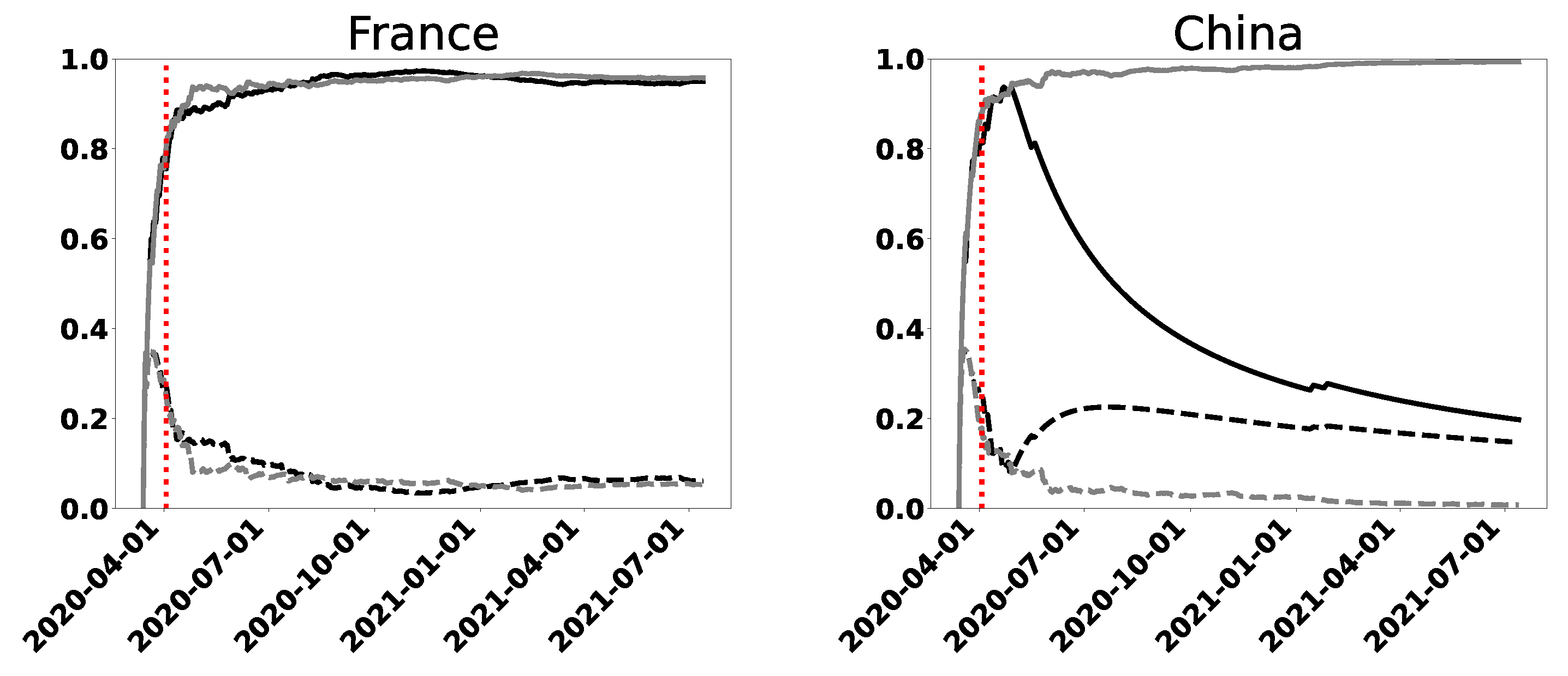
In Figure 1, we show the permutation entropy and statistical complexity for some chosen countries that provide a representative synthesis of the behaviors we found for all other nations. In addition, we depict the behavior for the world as a whole (the interested reader can find more information at the end of the article, where we show a larger set of countries, a total of 20). The graphs obtained for France (FRA) and the world are typical of most developed and developing countries. Australia (AUS), China (CHN), and some other countries exhibit a somewhat atypical behavior and will be discussed in detail separately. Notice that we use ISO-3166 alpha-3 country codes; for details, see https://www.iso.org/iso-3166-country-codes.html (accessed on 4 August 2021). In Figure 1 we plot the time dependence of the normalized permutation entropy $H\left(t\right)$ and of the statistical complexity $C\left(t\right)$. This is carried out for the statistics of daily new confirmed infected cases and daily new deaths.

In Figure 1 it can be seen that, about 60 days after 11 March 2020, entropy curves end their fast growth and begin to flatten (a similar conclusion can be reached studying other countries, as will be shown below). This would make it reasonable to determine the minimum length N, for the following method, where intervals of equal length are used. We take intervals with $N\ge 64$ data. This particular number is chosen for the sake of comparison with wavelet results.

The first important characteristic we observe in all cases shown is a high entropy value for $t\ge 64$, regarding infections as well as deaths. We observe that $H\left(t\right)>0.9$ and increases in time to values even very close to the maximum value 1, at least in 2020. These results exhibit a marked lack of information, i.e., a high degree of randomness. Across the world, this phenomenon is observed. Perhaps, in some cases, it might be related to the capability of collecting robust statistical data. However, it might also reflect differences in the dynamics of the spread of COVID-19.

Another peculiarity that we can conclude by looking at the entropy plots is that the general trend is: more data imply less information, i.e., $H\left(t\right)$ is always increasing. This fact would indicate the difficulty of predictive mathematical methods that could be used, even in the case of those models with stochastic components. Let us remember that our analyses are based only on the data series of infected and deceased people. Of course, if concrete information is supplemented (such as mobility data, contagion factor, etc.), many inferences could be made for decision-making policies. However, our point here is that the high entropy values computed reflect the fact that it was difficult to infer the dynamics of the coronavirus disease by just looking at the considered curves, and that modeling such dynamics was a challenge, as reflected in some works from the analyzed period.

Another possible use of this type of analysis is to measure the fidelity of the original data series. By common sense, one expects that the data corresponding to the deaths will be more reliable than those of infected cases. This means lower entropy for death cases. We can use the two available curves, for infected (IC) and death (DC) cases, to obtain more information about the treatment in each country. For our conclusions, we will consider goodwill in the data upload. In general, we expect the IC curves to be above the DC curves for a correct data collection, but: (1) the gap between curves has importance. Greater distance between curves can represent an incorrect collection of infected cases or a good collection of data on deaths. However, in the context studied, we interpret that this result implies a good collection of data on deaths. (2) If the DC curve is slightly above or below or coincides by parts with the IC one, it can be considered that the test is likely the adequate.

Most developed and developing countries show similar IC and DC curves, which are also similar to those for the world taken as a whole (corresponding to situation 2, with small differences between the values of the IC and DC curves).

It is seen from the plots that Australia, China, Cuba, and New Zealand (NZL) exhibit a different behavior between the curves corresponding to infected and death cases, starting from approximately the day $N=64$ (12 May 2020)—that is, from the value of N (or t) for which we consider the method reliable. The normalized entropy $H\left(t\right)$ corresponding to the DC curves is below that of IC ones, by a factor of around 0.3. Therefore, DC curves contain more information than IC ones. The analysis corresponding to these countries corresponds to situation 2. Additionally, the entropy DC curve for Australia has decreased monotonously since October 2020, which is an improvement in the information level of the pandemic. This behavior coincides with a decrease observed in the same period, in the original series of data on deceased people. Finally, we observe that Congo has marked differences from the mentioned countries, which may suggest that the data were not correctly recorded in that case. This happens not only for this country but also for some others in Central America or Central Africa, and for small islands.

The curves for complexity go along with the growth of the entropies until the complexity reaches its absolute maximum and then they decrease, moving away from the entropy curves towards small values that must also be associated with randomness. This change in behavior occurs around $D!=24$ (3 April 2020). The effect is produced because the disequilibrium Q compensates the growth of the entropy up to that point, but then it is overcome. The growth of $H\left(t\right)$ is noticeable and then it cannot compete. Perhaps one might think that the length of these intervals (and intervals with the same length), where both quantifiers are competitive, is the only reliable ones for making predictions. Similar plots are obtained starting from any day as long as the interval has $N\ge 4$ points.

The results obtained for $H\left(t\right)$ are all confirmed by those of complexity $C\left(t\right)$. Moreover, it can be said that, in this problem, the complexity is virtually determined by the behavior of the entropy, with such large values and with such a speed of growth. For this reason, from here on, we concentrate on the plots for entropies.

Thus, for the countries with typical behavior, the values are very small $C\left(t\right)<0.2$, while in those special ones, it grows and decreases according to the entropy decrease and growth, showing, in some cases, some degree of complexity.

We notice the following remarkable facts: (1) most of the countries that appear in the OWID database (which we have examined) show the same characteristics listed above; (2) the curves corresponding to the daily infected data are similar, despite the different geographical and cultural characteristics, different seasons, and applied health policies; and (3) something similar happens with the daily deaths curves, except in some special countries to which we have referred to.

This makes us think that what the monotonically increasing curves is a representation of the intrinsic or inherent form of spread of the SARS-CoV-2 virus, in terms of entropy (mainly IC curves). Therefore, we could choose, for example, the curve corresponding to the whole World, showed in Figure 1, as the model.

The deviations from the monotonically increasing curve of a country, coincide with a decrease in the cases publicly communicated by the respective government and registered in the OWID database.

Naturally, it has been thought that the decrease in cases correspond to effective health policies applied by the governments (among other causes) in the previous period to the massive use of anti-COVID vaccines.

4.2. Rolling Windows

The golden rule in series analysis is to compare series of the same interval length, but as mentioned before, there was not enough data available for the period considered to draw reliable conclusions. We consider here another way to see the development of the quantifiers as a function of time. Unlike the treatment given in Section 4.1, we now keep constant the intervals length, but these are not consecutive and share data. We do this by using so-called rolling or sliding windows. A similar analysis is conducted in [8,9], for time series of financial data using permutation entropy.

Here, we employ the rolling windows method for the permutation method and the wavelet transform. We will consider intervals (windows) of three different lengths. As we want to carry out a comparative analysis between the permutation and wavelet entropies, these lengths will be $N=256$, $N=128$ and $N=64$, which arise because wavelet analysis require intervals of length $2^j$, with $jϵ\mathbb{N}$ (see Section 3.2). In wavelet decomposition of these series, the maximum number of scales were considered (corresponding to 6, 7, and 8 scales, respectively) and detail coefficients were used to calculate wavelet energy.

The analysis will be conducted only for the entropies (2). We will proceed to take consecutive windows $[n,n+N]$, with $n=0,1,\cdots W_n$, $W_n$ being the maximum number of intervals that fit in the total number of data of the original series, according to the value of N. Thus, we will obtain values for the entropies of the considered windows. Of course, we can associate these windows with the corresponding days-dates. We will take as the first day 11 March 2020 and we will consider data until 13 July 2021.

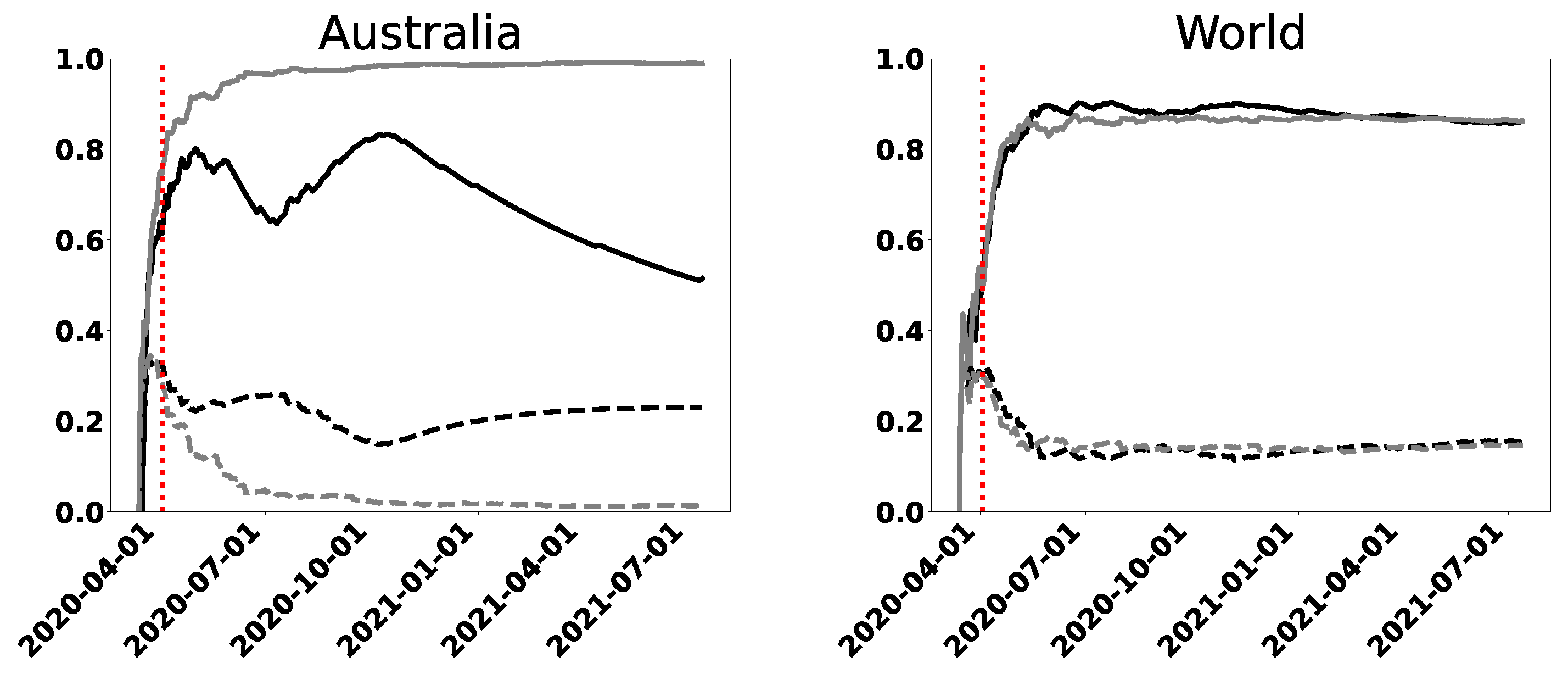
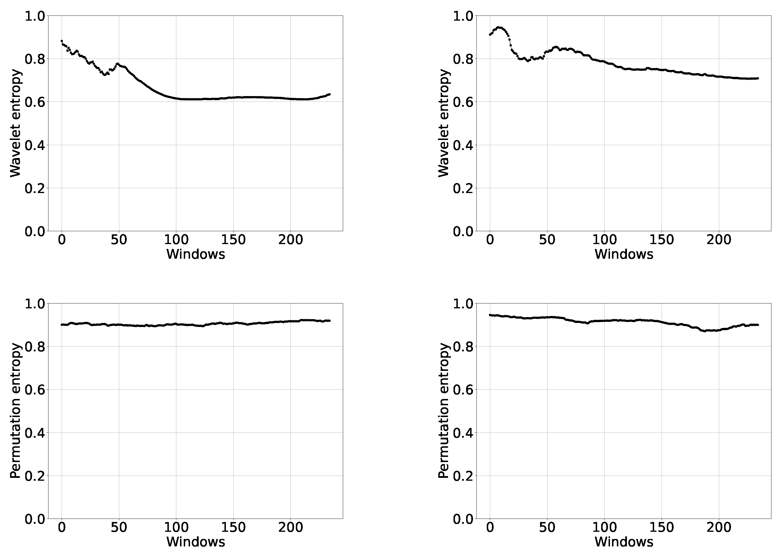
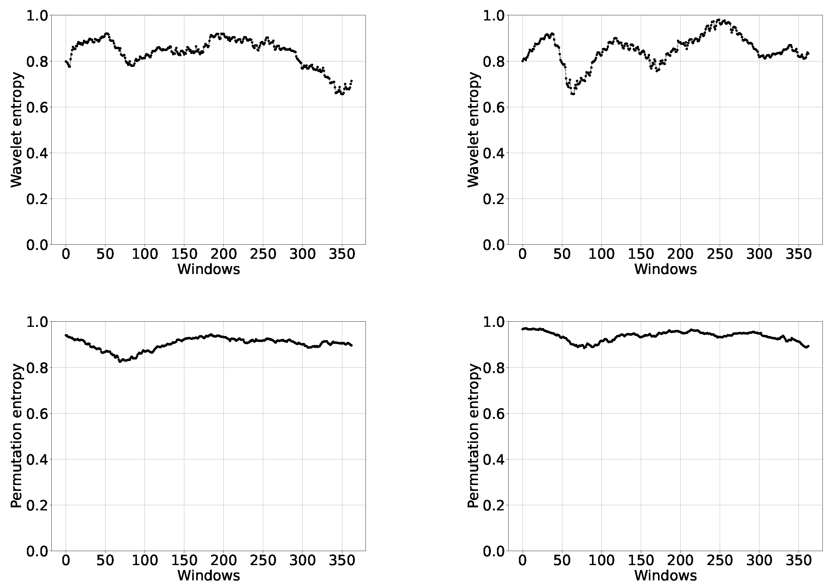
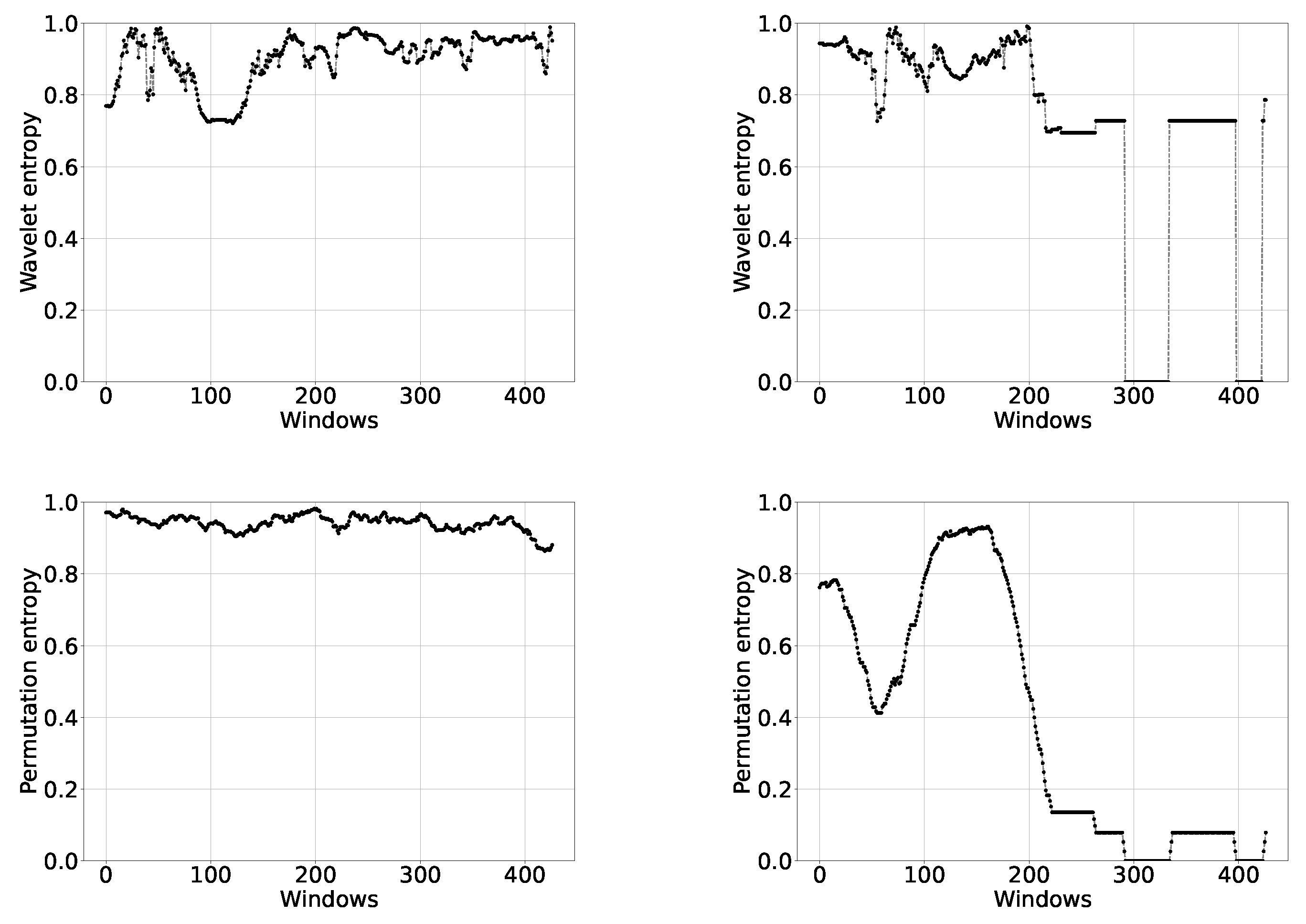
Representative examples of the results are shown in the following plots. In Figure 2, Figure 3 and Figure 4, we depict the IC and DC curves of wavelet and permutation entropies, with rolling windows of different lengths. The figures correspond, respectively, to the United States of America (USA) with $N=256$, Brazil (BRA) with $N=128$, and Australia with $N=64$.

The first thing to observe in these figures is a difference in shape with respect to the curves corresponding to increasing intervals. This not only happens with wavelet entropies, as one thinks at first, but also with permutation ones. Obviously, an information quantifier based on the permutation methodology, in general, does not have to give the same result as the corresponding quantifier evaluated using the wavelet transform. The first method takes account of causality, while the second one provides a general representation in time and frequency. What one expects to find in the main characteristics of the problem is coherence between both methodologies. On the other hand, we have observed that, if we look at the figures corresponding to increasing intervals, but from the value 64, they are consistent with those of rolling windows with $N=256$, which represent a large amount of points as can be seen in Figure 2, thus throwing a good result.

The differences between the curves for wavelet and permutation entropies can be observed in Figure 2, Figure 3, Figure 4, Figure 5 and Figure 6. We can see that the wavelet entropy values in general are lower than the permutation, although they are also very high. This is the main coherence that interests us in this article.

We note in Figure 2, Figure 3 and Figure 4 a distinction between the IC and DC curves, for both wavelet and permutation entropies. It can also be observed that the fluctuations increase when N decreases and that they are greater in the wavelet framework. The curves for USA in Figure 2 ($N=256$) appear to show a slight but constant increase in information for the wavelet entropy, a result that is not accompanied by the permutation entropy. Once again, Australia shows an increase in information since the end of 2020, reaching zero when $N=64$ is taken for the length of the rolling windows (see Figure 4).

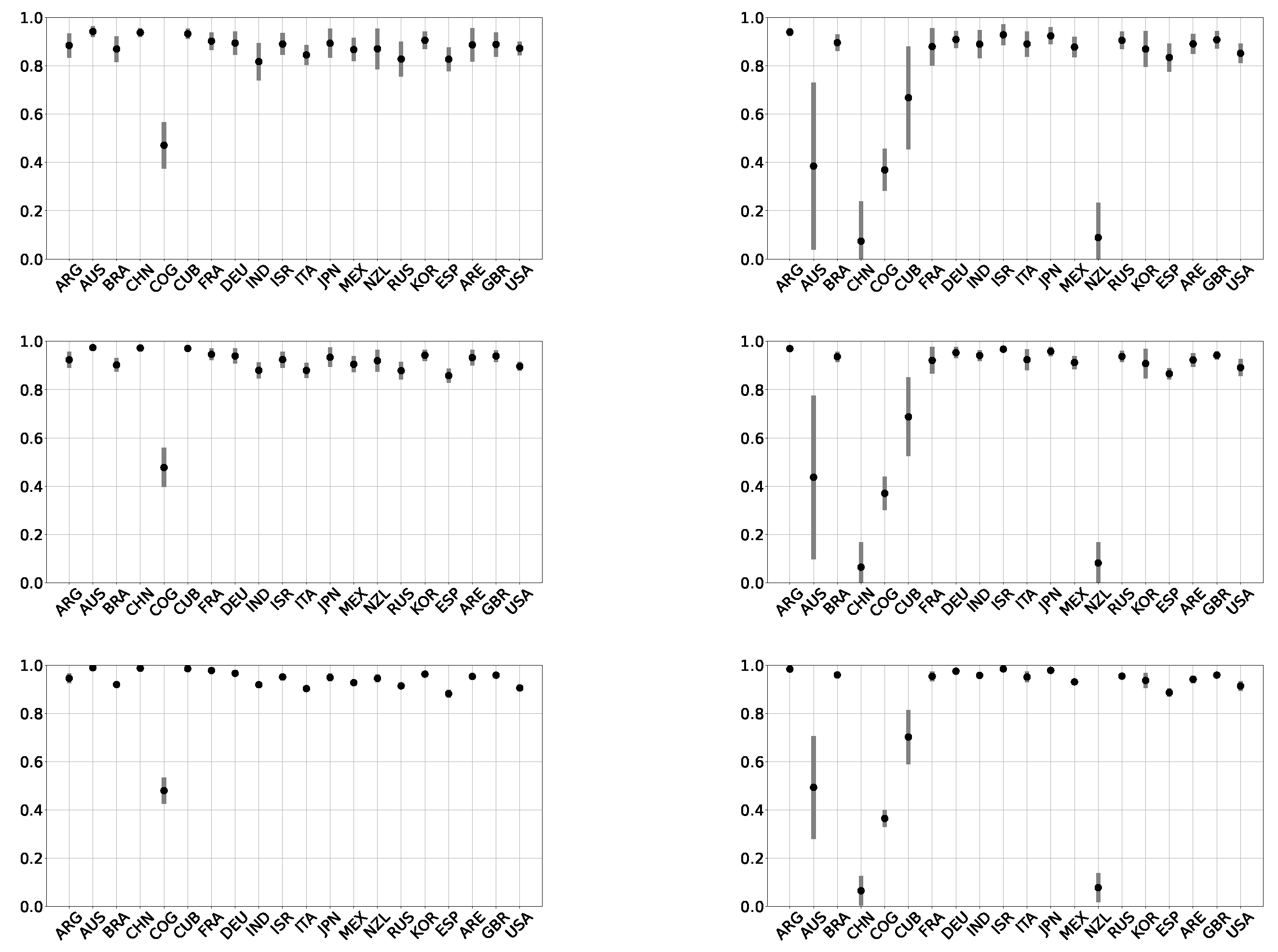
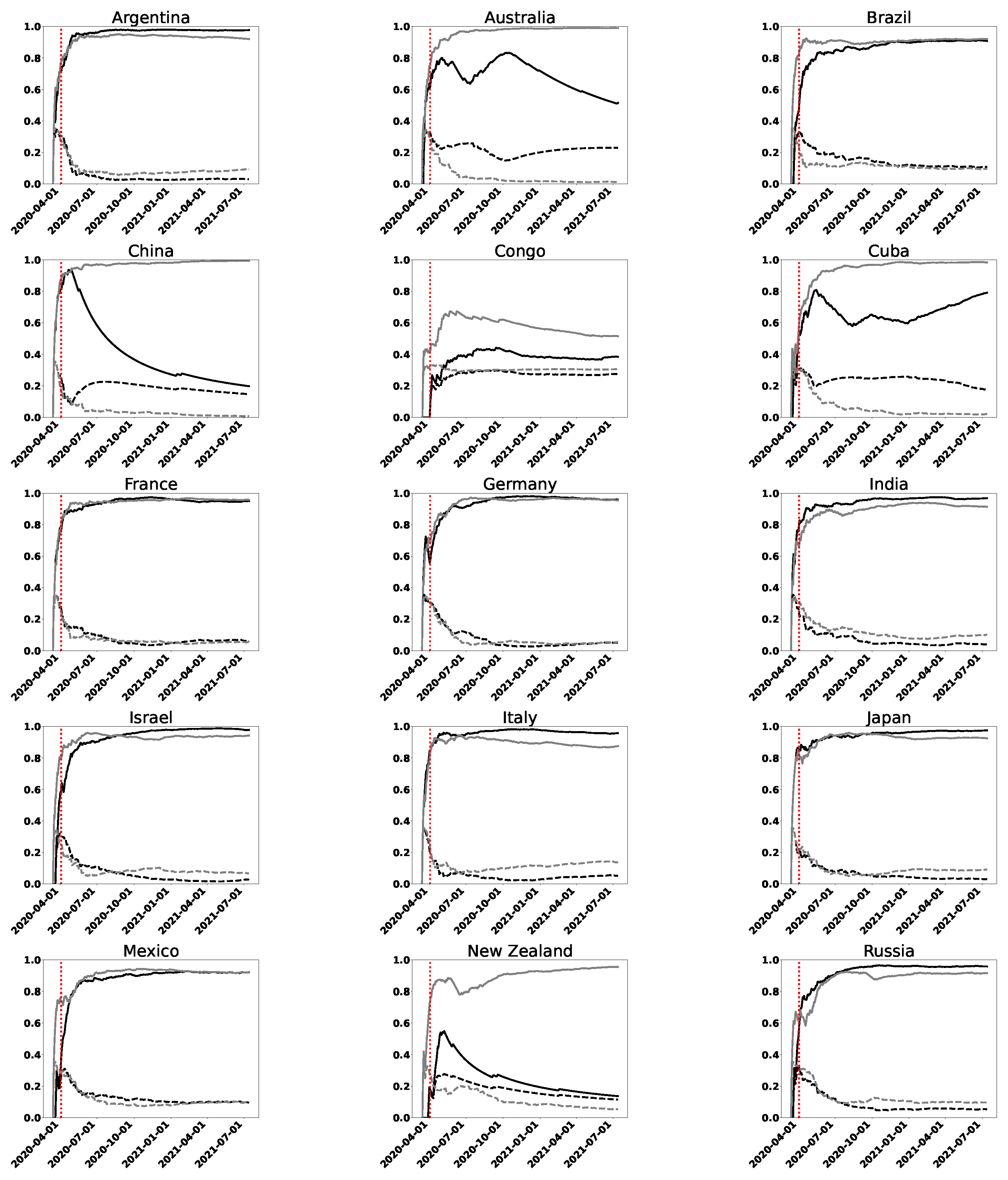
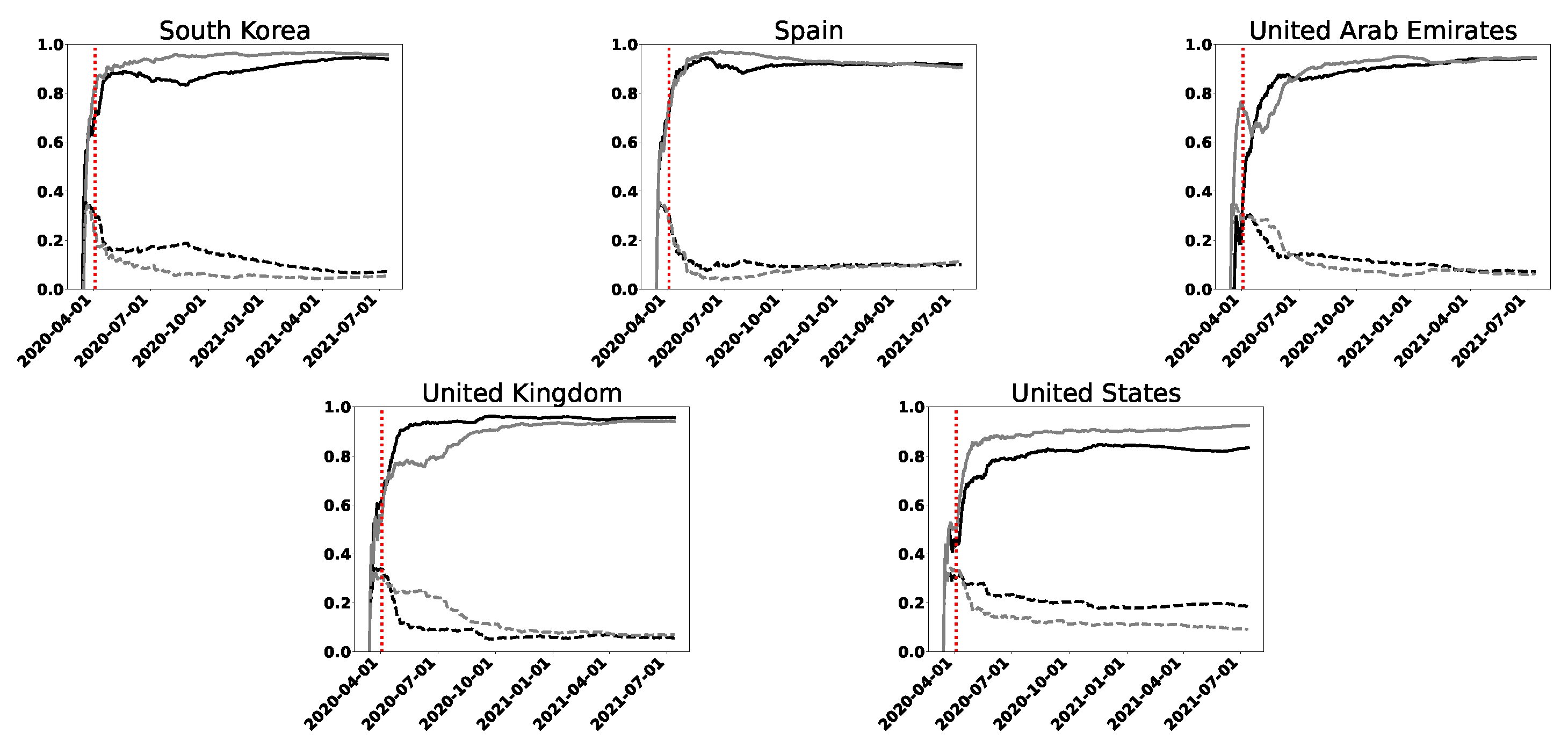
We exhibit in Figure 5 and Figure 6 a series of results for a set of 20 chosen countries (they are identified with their ISO-3166 alpha-3 code and appear in the same order—alphabetic by name—as in Figure 7). In Figure 5, which corresponds to the wavelet analysis, we see that entropy mean values are greater than 0.7 for both infected and death cases, except for some particular countries. Standard deviations remain below 0.2. For the permutation procedure, shown in Figure 6, we see that, for infected cases, the entropy mean values remain above 0.8 and mostly close to 1. In the DC curves, we observe that the mean values are grouped close to their maximum value, except for Australia, China, Cuba, and New Zealand, showing standard deviations greater than those of all the other countries studied. Both IC and DC curves have the characteristic of maintaining the relative differences between their values when N is changed.

All of our analysis leads to the expected result, but in a notorious way that the curves corresponding to the daily deaths may contain much more information than the infected curves. Australia and New Zealand are good examples of this. According to what is observed in the registered cases, the DC curves would show a better description with respect to the pandemic.

Finally, we must mention Israel, a country for which, in Figure 7, there is no increase in information towards the last days considered (mid-July), when there was a drastic decrease in mortality. However, in the graphs corresponding to $N=64$ calculated with the rolling windows method, a significant increase in information is observed for a short time, until a decrease is noted again, probably due to a new virus variant. This could happen with some other country and is a consequence of the large number of points accumulated in the increasing intervals of Figure 7.

5. Conclusions

The main goal of this article has been to look for reliable information contained in the daily data series corresponding to the COVID-19 pandemic produced by the SARS-CoV-2 virus. We have considered the information concerning infected and deceased cases. The source for this study was the Our World in Data COVID-19 database [36].

We have taken as the first day 11 March 2020, and considered data until mid July 2021. Obviously, the total interval considered includes several waves, but we do not analyze these phenomena. Our investigations focus on the pre-vaccination period, as this is the time interval with the greatest randomness in the available data. In this period, the infection had the greatest ability to show its intrinsic dynamics, tempered by the well-known interventions of world governments through their health policies (mainly lockdown). We have studied the pandemic as a whole, including some countries where the increase in information has been of considerable amount. We have detected that this fact coincides with a decrease in cases.

For this analysis, we have mainly used the normalized entropy (2), but in certain cases, the normalized statistical complexity (4) also showed its usefulness. To compute these information quantifiers, we have employed the probability distribution functions given by the Bandt–Pompe permutation method and by a wavelet transform. In the permutation case, we have taken $D=4$ and $\tau =1$, and we have also varied these parameters verifying consistency. Moreover, we have considered intervals of length $N\ge 64$. This particular number is chosen in order to compare results with wavelet analysis. For the wavelet-based PDFs, a discrete wavelet transform with the orthogonal wavelet function db10 was used. Possibly, the use of this type of graph ($N=64$) allows for analyzing the waves in each country.

To study the temporal evolution of the pandemic, we cannot take, as usual, consecutive temporal intervals of the same length, which is done for comparison purposes. The lack of a sufficient amount of data from the series in the period considered led us to use methods other than the usual one. We have considered two ways of treating the data. We employed (1) increasing intervals and (2) intervals of fixed length (rolling, or sliding, windows). The former shows a global view of the pandemic, while the rolling windows’ technique shows a more local description, especially for smaller intervals—in this case, for $N=64$.

In the increasing intervals case, only the permutation methodology has been used to determine the respective PDFs. In the second one, we have also performed a wavelet analysis. For the rolling windows technique, we have used fixed length intervals of $N=$ 64, 128, and 256 points, to be able to compare results between both methods.

We have implemented our approach for every country in the world and made detailed analyses. In this contribution, for brevity, we show a set of representative examples.

The results obtained with each method have differences, but they show consistency in the main results. It is obvious that one cannot expect both methods to yield exactly the same results. The permutation method looks for causality, while the wavelet one provides a general representation in time and frequency. Notwithstanding this, both strategies throw high entropic values for most time intervals and countries, indicating a general lack of information in the collected data. The comparison between Figure 5 and Figure 6 suggest that the permutation entropy method brings a better representation of the problem.

In both cases, the normalized entropy attains high values, greater than $0.8$ mostly and even close to 1 in some situations. This represents a high degree of randomness which brings us to the main result of the article: the lack of information contained in the pandemic data series. It is worth stressing that both methodologies used here coincide in this respect. This fact would indicate the difficulties of the predictive mathematical approaches in the analyzed period if only the information contained in the data series corresponding to the cases of infected and deceased people is used. Concomitant information should be added, such as mobility data, contagion factor, etc. On the other hand, local structures and interactions could be analyzed.

In Figure 1 and Figure 7, we represent $H\left(t\right)$ and $C\left(t\right)$ defined for increasing intervals. It is observed that, with some exceptions, the IC entropy is an increasing function of t. The more points we have, the greater the entropy. The growth is such that it exceeds the disequilibrium factor Q quickly before the reliable region. Although complexity is not a function of entropy, it is, in this case, clearly subordinate to it. Most developed and developing countries show similar behavior but Australia, New Zealand, China, and Cuba exhibit a different behavior between both types of curves (IC and DC). The entropy corresponding to the DC curves has lower values than that of the IC ones. A fall in the value of the DC entropy for Australia can be observed towards the end of 2020 and the beginning of 2021, when we talk about DC curves. The last characteristic is maintained in the rolling windows figures for permutation and wavelet analysis (Figure 2, Figure 3, Figure 4, Figure 5 and Figure 6).

Our research leads to an expected but notorious result in special situations in which the curves corresponding to the daily new deaths may contain much more information than the IC curves. This happens, for example, for Australia, New Zealand, and China. They would show a better behavior, with respect to the pandemic.

We have also mentioned the similarity between graphs for the 207 countries studied, in the case of the increasing intervals methodology and for the infected curves. This fact naturally led us to think that, in terms of entropy, what we had found is a representation of the intrinsic propagation curve for the SARS-CoV-2 virus.

Summing up, we have introduced a methodology based on entropic information quantifiers to know how much information is really available in worldwide data series corresponding to the COVID-19 pandemic. We have found that it is generally very low, which is indicative of a highly random process. This renders the predictions by mathematical models difficult. As a second result, we have seen that it can be used to compare the behavior of different countries and to test the quality and reliability of data on the pandemic. Finally, we have seen that the methodology has been able to detect a decrease in the effects of the coronavirus disease pandemic, by observing an increase in the information contained in the corresponding data.

References

- James, L.P.; Salomon, J.A.; Buckee, C.O.; Menzies, N.A. The use and misuse of mathematical modeling for infectious disease policymaking: Lessons for the COVID-19 pandemic. Med. Decis. Mak. 2021, 41, 379–385. [Google Scholar] [CrossRef]
- Loève, M. Probability theory II. In Graduate Texts in Mathematics, 4th ed.; Springer: Berlin/Heidelberg, Germany, 1978; Volume 46. [Google Scholar]
- Falsone, G.; Laudani, R. Probability transformation method for the evaluation of derivative, integral and Fourier transform of some stochastic processes. J. Eng. Math. 2021, 131, 12. [Google Scholar] [CrossRef]
- Türkşen, I.B. (Ed.) Chapter 1—Introduction. In An Ontological and Epistemological Perspective of Fuzzy Set Theory; Elsevier Science: Amsterdam, The Netherlands, 2006; pp. 55–75. [Google Scholar]
- Kowalski, A.M.; Rossignoli, R.D.; Curado, E.M.F. (Eds.) Concepts and Recent Advances in Generalized Information Measures and Statistics; Bentham Science Publishers: Sharjah, United Arab Emirates, 2013. [Google Scholar]
- Shannon, C.E. A Mathematical Theory of Communication. Bell Syst. Tech. J. 1948, 27, 379–423. [Google Scholar] [CrossRef] [Green Version]
- Zanin, M.; Zunino, L.; Rosso, O.A.; Papo, D. Permutation entropy and its main biomedical and econophysics applications: A review. Entropy 2012, 14, 1553–1577. [Google Scholar] [CrossRef]
- Henry, M.; Judge, G. Permutation entropy and information recovery in nonlinear dynamic economic time series. Econometrics 2019, 7, 10. [Google Scholar] [CrossRef] [Green Version]
- Arouxet, M.B.; Bariviera, A.F.; Pastor, V.E.; Vampa, V. COVID-19 impact on cryptocurrencies: Evidence from a wavelet-based Hurst exponent. Physica A 2022, 596, 127170. [Google Scholar] [CrossRef]
- Zozor, S.; Portesi, M.; Lamberti, P.W.; Bosyk, G.M.; Bercher, J.-F. Special Issue “Entropies, Divergences, Information, Identities and Inequalities”. Entropy 2022. [Google Scholar]
- Li, X.; Ouyang, G.; Richards, D. Predictability analysis of absence seizures with permutation entropy. Epilepsy Res. 2007, 77, 70–74. [Google Scholar] [CrossRef]
- Ouyang, G.; Li, J.; Liu, X.; Li, X. Dynamic characteristics of absence EEG recordings with multiscale permutation entropy analysis. Epilepsy Res. 2013, 104, 246–252. [Google Scholar] [CrossRef]
- Kumar, M.; Pachori, R.; Acharya, U. Automated diagnosis of myocardial infarction ECG signals using sample entropy in flexible analytic wavelet transform framework. Entropy 2017, 19, 488. [Google Scholar] [CrossRef]
- Valverde, E.; Clemente, G.; Arini, P.; Vampa, V. Wavelet-based entropy and complexity to identify cardiac electrical instability in patients post myocardial infarction. Biomed. Signal Process. Control 2021, 69, 102846. [Google Scholar] [CrossRef]
- Shiner, J.S.; Davison, M.; Landsberg, P.T. Simple measure for complexity. Phys. Rev. E 1999, 59, 1459. [Google Scholar] [CrossRef]
- López-Ruiz, R.; Mancini, H.; Calbet, X. A statistical measure of complexity. Phys. Lett. A 1995, 209, 321–326. [Google Scholar] [CrossRef] [Green Version]
- Kowalski, A.M.; Martín, M.T.; Plastino, A.L.; Proto, A.; Rosso, O.A. Wavelet statistical complexity analysis of classical limit. Phys. Lett. A 2003, 311, 180–191. [Google Scholar] [CrossRef]
- Kowalski, A.M.; Martín, M.T.; Plastino, A.; Rosso, O.A. Bandt–Pompe approach to the classical-quantum transition. Physica D 2007, 233, 21–31. [Google Scholar] [CrossRef]
- Kowalski, A.M.; Plastino, A.; Rossignoli, R. Complexity of a matter-field Hamiltonian in the vicinity of a quantum instability. Physica A 2019, 513, 767–774. [Google Scholar] [CrossRef] [Green Version]
- Calbet, X.; López-Ruiz, R. Tendency towards maximum complexity in a nonequilibrium isolated system. Phys. Rev. E 2001, 63, 066116. [Google Scholar] [CrossRef] [Green Version]
- Sanchez, J.R.; López-Ruiz, R. A method to discern complexity in two-dimensional patterns generated by coupled map lattices. Physica A 2005, 355, 633–640. [Google Scholar] [CrossRef] [Green Version]
- López-Ruiz, R. Complexity in some physical systems. Int. J. Bif. Chaos 2001, 11, 2669–2673. [Google Scholar] [CrossRef] [Green Version]
- Crutchfield, J.P.; Young, K. Inferring statistical complexity. Phys. Rev. Lett. 1989, 63, 105–108. [Google Scholar] [CrossRef]
- Rosso, O.A.; Larrondo, H.A.; Martín, M.T.; Plastino, A.L.; Fuentes, M.A. Distinguishing Noise from Chaos. Phys. Rev. Lett. 2007, 99, 154102. [Google Scholar] [CrossRef] [PubMed]
- Zunino, L.; Zanind, M.; Tabake, B.M.; Pérez, D.G.; Rosso, O.A. Complexity-entropy causality plane: A useful approach to quantify the stock market inefficiency. Physica A 2010, 389, 1891–1901. [Google Scholar] [CrossRef] [Green Version]
- Lamberti, P.W.; Martín, M.T.; Plastino, A.L.; Rosso, O.A. Entropic nontriviality measure. Physica A 2004, 334, 119–131. [Google Scholar] [CrossRef]
- Rosso, O.A.; Micco, L.D.; Larrondo, H.A.; Martín, M.T.; Plastino, A.L. Generalized statistical complexity measure. Int. J. Bif. Chaos 2010, 20, 775–785. [Google Scholar] [CrossRef]
- Rosso, O.A.; Craig, H.; Moscato, P. Shakespeare and other English renaissance authors as characterized by information theory complexity quantifiers. Physica A 2009, 388, 916–926. [Google Scholar] [CrossRef]
- Rosso, O.A.; Blanco, S.; Jordanova, J.; Kolev, V.; Figliola, A.; Schürmann, M.; Başar, E. Wavelet entropy: A new tool for analysis of short duration brain electrical signals. J. Neurosc. Methods 2001, 105, 65–75. [Google Scholar] [CrossRef]
- Rosso, O.A.; Mairal, L. Characterization of time dynamical evolution of electroencephalographic records. Physica A 2002, 312, 469–504. [Google Scholar] [CrossRef]
- Bandt, C.; Pompe, B. Permutation entropy: A natural complexity measure for time series. Phys. Rev. Lett. 2002, 88, 174102. [Google Scholar] [CrossRef]
- Rosso, O.A.; Micco, L.D.; Plastino, A.L.; Larrondo, H.A. Info-quantifiers’ map-characterization revisited. Physica A 2010, 389, 4604–4612. [Google Scholar] [CrossRef]
- Blanco, S.; Figliola, A.; Quiroga, R.Q.; Rosso, O.A.; Serrano, E. Time-frequency analysis of electroencephalogram series. III. Wavelet packets and information cost function. Phys. Rev. E 1998, 57, 932. [Google Scholar] [CrossRef]
- Gamero, L.; Plastino, A.L.; Torres, M.E. Wavelet analysis and nonlinear dynamics in a nonextensive setting. Physica A 1997, 246, 487–509. [Google Scholar] [CrossRef]
- Chui, C.K. An Introduction to Wavelets; Academic Press: New York, NY, USA, 1992. [Google Scholar]
- Ritchie, H.; Ortiz-Ospina, E.; Beltekian, D.; Mathieu, E.; Hasell, J.; Macdonald, B.; Giattino, C.; Appel, C.; Rodés-Guirao, L.; Roser, M. Coronavirus Pandemic (COVID-19). 2020. Available online: https://www.ourworldindata.org/coronavirus (accessed on 3 August 2021).
- Ouyang, G. Permutation Entropy. MATLAB Central File Exchange. 2021. Available online: https://www.mathworks.com/matlabcentral/fileexchange/37289-permutation-entropy (accessed on 23 June 2021).
- Daubechies, I. Ten lectures on wavelets. In CBMS-NSF Regional Conference Series in Applied Mathematics; Society for Industrial and Applied Mathematics: Philadelphia, PA, USA, 1992. [Google Scholar]
Figure 1.
Permutation entropy (full line) and permutation statistical complexity (dashed line), as functions of time, for three representative countries and the whole world. The curves correspond to infected (gray line) and death (black line) cases. We consider increasing intervals measured from a fixed initial date (11 March 2020) and with increments of one day until 13 July 2021. The vertical dashed line corresponds to .
Figure 2.
Wavelet entropy (upper row) and permutation entropy (lower row) vs. windows, with rolling windows of length , for infected (left) and death (right) cases in the United States. We consider cases reported from 11 March 2020 until 13 July 2021.
Figure 3.
Wavelet entropy (upper row) and permutation entropy (lower row) vs. windows, with rolling windows of length , for infected (left) and death (right) cases in Brazil. We consider cases reported from 11 March 2020 until 13 July 2021.
Figure 4.
Wavelet entropy (upper row) and permutation entropy (lower row) vs. windows, with rolling windows of length , for infected (left) and death (right) cases in Australia. We consider cases reported from 11 March 2020 until 13 July 2021.
Figure 5.
Mean values and standard deviations of the wavelet entropy using rolling windows, for daily infected cases (left) and daily deaths (right). We consider fixed windows of length (upper row), (middle row), and (lower row), for 20 countries (the country codes follow ISO-3166 alpha-3 standards). We consider cases reported from 11 March 2020 until 13 July 2021.
Figure 6.
Mean values and standard deviations of the permutation entropy using rolling windows, for daily infected cases (left) and daily deaths (right). We consider fixed windows of length (upper row), (middle row), and (lower row), for 20 countries (the country codes follow ISO-3166 alpha-3 standards). We consider cases reported from 11 March 2020 until 13 July 2021.
Figure 7.
Permutation entropy (full line) and permutation statistical complexity (dashed line), as functions of time, for the set of 20 countries considered in Figure 5 and Figure 6. The curves correspond to infected (gray line) and death (black line) cases. We consider increasing intervals measured from a fixed initial date (11 March 2020) and with increments of one day until 13 July 2021. The vertical dashed line corresponds to .
Publisher’s Note: MDPI stays neutral with regard to jurisdictional claims in published maps and institutional affiliations. |
© 2022 by the authors. Licensee MDPI, Basel, Switzerland. This article is an open access article distributed under the terms and conditions of the Creative Commons Attribution (CC BY) license (https://creativecommons.org/licenses/by/4.0/).
Share and Cite
MDPI and ACS Style
Kowalski, A.M.; Portesi, M.; Vampa, V.; Losada, M.; Holik, F. Entropy-Based Informational Study of the COVID-19 Series of Data. Mathematics 2022, 10, 4590. https://doi.org/10.3390/math10234590
AMA Style
Kowalski AM, Portesi M, Vampa V, Losada M, Holik F. Entropy-Based Informational Study of the COVID-19 Series of Data. Mathematics. 2022; 10(23):4590. https://doi.org/10.3390/math10234590
Chicago/Turabian StyleKowalski, Andres M., Mariela Portesi, Victoria Vampa, Marcelo Losada, and Federico Holik. 2022. "Entropy-Based Informational Study of the COVID-19 Series of Data" Mathematics 10, no. 23: 4590. https://doi.org/10.3390/math10234590
Note that from the first issue of 2016, this journal uses article numbers instead of page numbers. See further details here.