
Adoption of Satellite Offices in Response to a Pandemic: Sustainability and Infection Control


1
College of Business Administration, Hongik University, Seoul 04066, Korea
2
Department of Engineering Management, Systems, and Technology, University of Dayton, Dayton, OH 45469, USA
3
College of Business, Hankuk University of Foreign Studies, Seoul 02450, Korea
*
Author to whom correspondence should be addressed.
Sustainability 2021, 13(14), 8008; https://doi.org/10.3390/su13148008
Submission received: 30 May 2021
/
Revised: 26 June 2021
/
Accepted: 13 July 2021
/
Published: 17 July 2021
(This article belongs to the Special Issue The Future of Facilities Management and Sustainable Development)
Abstract
:The office environment has changed rapidly due to the recent COVID-19 outbreak. Companies consider various types of remote work environments to contain the spread of the virus. Among them, a satellite office is a type of remote work environment where a number of employees are allocated to their nearest office. The benefits from satellite offices are twofold: The significant reduction of travel distance also reduces the amount of carbon emission and fuel consumption. In addition, dividing employees into smaller groups significantly reduces the potential risks of infection in the office. This paper addresses a satellite office allocation problem that considers social and environmental sustainability and infection control at work. In order to evaluate the effect of different satellite office allocation, quantitative measures are developed for the following three criteria: carbon emission, fuel consumption, and the probability of infection occurrence at work. Simulation experiments are conducted to investigate different scenarios of regional infection rate and modes of transportation. The results show that adopting satellite offices not only reduces carbon emission and fuel consumption, but also mitigates business disruption in the pandemic.
1. Introduction
The ongoing COVID-19 pandemic has drastically changed the office environment. To avoid being exposed to the virus and minimize close contacts, more and more people perform their job outside of the office, working remotely. Based on recent surveys conducted after the outbreak of the virus, about half of the workforce in the United States employed before COVID-19 is now working at home, and 35.2% recently switched from commuting to remote work [1]. Concepts of remote work are not completely new: it generally implies that a company’s normal operations are performed outside the normal organizational confines [2]. Thanks to advancements in telecommunication technology and office automation, traveling to the central work location has been substituted with various types of remote office work. Once catalyzed by the pandemic, however, these changes in work and employment environment may lead to a permanent shift that lasts beyond the pandemic.
Working outside of the office, remote work provides employees with a great deal of temporal and locational flexibility. Remote work options differ in scope and structure, depending on the employees’ commuting frequency. Among others, the satellite office is an intermediate form of remote work between working at home and commuting long distances, in which employees are relocated to their nearest satellite sites to reduce travel time [2,3,4]. The introduction of new technologies, such as teleconferencing, cloud computing, etc., to the office environment enables employees from different departments in the organization to occupy the building and share the space and equipment, lifting constraints in determining the location of the office building. In the era of the pandemic, many companies have started adopting satellite work site policies in effort to reduce the risks of keeping the critical mass of employees in a single location as well as risks of employees being exposed to the virus when commuting for a longer time [5].
From a facility management perspective, the COVID-19 pandemic becomes another huge challenge. Building management must ensure a healthy work environment to sustain the building occupants’ health and well-being in the face of the pandemic. For instance, a considerable amount of effort is required in cleansing and disinfection to reduce the transmission of the disease in the office. Sharing items or using sustainable products for the kitchen and bathroom is discouraged: they must be replaced by disposable items if applicable. In particular, limiting capacity in the office area is recommended or imposed by regulations so that risks of exposure to the virus can be restrained and physical distancing can be secured. A clear guideline must be put in place if a sick person is found in the building. To prevent further transmission of the virus, it is required to close off the areas that were used and occupied by the person or even the entire building for at least 24 hours or even longer until the cleaning and disinfecting are done [6]. Therefore, careful examination is required in determining the capacity of an office, considering both operating costs for running multiple sites with limited capacity and potential risks of closing off the office partially or entirely.
In this paper, we propose a facility capacity/location decision model to implement satellite office policies, considering sustainability and infection control. In response to the pandemic, the facility management’s decision is made not only to minimize operating costs but also to reduce infection and transmission of the virus both in the office and during employees’ commute. In the centralized office arrangement where all employees work in a single office location, there is a higher risk of the virus spreading among the employees. Once an employee’s infection is confirmed, the facility should be operated by numbers of people less than its full capacity: the office needs to be shut down for cleaning and disinfection of the area used by the sick person and any employees who made close contact with that person must self-quarantine for 14 days, working at home if possible [7]. In addition, workers are exposed to the virus for longer durations when traveling using public transportation. Driving a private car alone is highly recommended over public transportation to reduce such exposure. As more people turn to driving cars instead of using mass transit, however, it may lead to a surge in carbon emission from vehicles due to congestion.
Benefits from the implementation of satellite offices can be summarized as follows: a company can restrain the diseases for spreading by limiting the size of the office, thereby exponentially minimizing the probability of office shutdown. Employees can save their daily commuting time significantly by traveling to the nearest satellite office and hence protecting themselves from the virus. Reduction in employees’ traveling time leads to less carbon emission. Some employees may choose to walk to work or use a bike instead of a car trip as they are now assigned to an office nearby. In those cases, the overall carbon footprint decreases even more, while they still can minimize the infection without using a private vehicle. Thus, the adoption of satellite offices will ensure employees’ health and wellness, which should be considered first and foremost in regard to organizational sustainability [8]. It will also enable the company to recognize social responsibilities for the neighborhood and community to contain the spread of the virus during the pandemic.
The purpose of this study is to determine the capacity and location of satellite offices, not only just to minimize fixed and operating costs, but also to reduce the probability of infection and transmission of the virus as well as the carbon emission from vehicles while traveling. To the best of our knowledge, no study considers the facility location problem in regard to sustainability and infection control.
The main contributions of this study are as follows:
- As far as we understand, this paper is the first which addresses the location-allocation problem for a company’s satellite office setup.
- A simulation model finds the decision regarding the assignment of employees from the headquarter to their nearest workspace and the capacity of each office will minimize travel time and thereby minimize carbon emission costs.
- The proposed model also estimates the infection probability at the office, which is imperative for business continuity as well as the employees’ health and safety during the COVID-19 pandemic.
- The results further suggest that given the rate of active cases of the infection around the region, the company can make decisions on the satellite offices’ policies by considering the infection probability accordingly.
- The above two contributions combined provides a risk management tool so that the company can take actions in any infection scenario ahead of time.
- The nature of the obtained solution is also studied.
The remainder of this paper is organized as follows: Section 2 presents the background of the different concepts of satellite office arrangements. Section 3 proposes the satellite office decision-making model. Section 4 demonstrates the numerical experiment and its results. Finally, conclusions are drawn in Section 5.
2. Research Background
There are different types of remote work, such as neighborhood work centers, client-based work, and shared-facility centers, to provide locational and temporal flexibility for workers [2,9,10]. Full debate on the taxonomy of remote work can be referred to in Ref. [11]. Satellite office or satellite work center, hereafter satellite office, is a term used for a specific type of remote work arrangement where work centers are located “in residential areas or in rural villages, owned by a specific company which has relocated part of its operations at a distance from an original or main site [10].” As an intermediate form of remote work between working at home and traveling to the main office, satellite office is distinct from other types of remote work in its hierarchical structure. With satellite offices, a company still can benefit from economies of scale; the number of employees on site is typically as many as several hundred [2].
The primary goal of almost all types of remote work is to significantly reduce the employee’s commute time and expenses [2,9], which may lead to affecting the employees’ psychological well-being and work-life balance. Overall, discussions on the benefits and effects of remote work for both the company and the individuals are mainly about (1) the time and expense of travel, (2) the work-life balance and job satisfaction of the employees, and (3) ability and performance of employees [12,13,14,15]. In the era of the pandemic, however, the discussion has been further extended to the safety and health crisis and risk management of the organization [5]. In the face of the COVID-19 crisis, companies must ensure their employees’ safety and health by managing risks of new infection from the workplace. These risks and its management must be considered so as to maintain the economic activity of the company and the individuals [16]. In this research, therefore, the objective of the implementation of satellite offices is to significantly contribute to the risk management of companies and sustain employees’ health and safety during the COVID-19 pandemic, while reducing traveling time and expenses.
Determining the location and capacity of satellite offices can be considered as a branch of the facility location-allocation problem where employees travel to their assigned satellite offices. Since the facility location-allocation problem was first introduced [17], most of the previous studies on the supply chain location-allocation problems have been concerned with the mathematical modeling of different approaches to obtain optimal decisions on transportation, inventory management, and production practices [18]. As the effects of pollution control and environmental considerations become more important to incorporate supply chain decisions, however, the facility network and carbon footprint decisions have been at the forefront of strategic decisions for the company. The majority of literature with environmental concerns target one or more of the following: (1) network design with carbon footprint, (2) emissions from production and transportation, and (3) greenhouse gas (GHG) and hazardous regulations [19,20,21]. A more detailed discussion on sustainable supply chain design can be found in Ref. [22].
In this paper, we consider a satellite office location-allocation problem where satellite office location and capacity will be determined not only to minimize travel time and carbon emission but also to minimize infection and the likelihood of transmission of the virus at work. Since distancing is required to mitigate the spread of the virus, the capacity of satellite offices must be determined so that distancing is possible. It must also be considered that when the size of an office is large and more employees are assigned to the same site, the infection probability will increase and the likelihood of closing off the area used by a sick employee or shutting down the entire office will also increase. According to the work by the Georgia Tech team, providing estimates of the risk, this probability is calculated with two factors: the location of offices and the size of the office [23]. A simulation model is proposed to calculate the infection probability as well as travel time/cost and carbon emission in different scenarios. The experiment results provide valuable explanation for potential exposure and infection, depending on the size and the number of satellite offices, which is imperative to corporate risk management planning in the pandemic.
3. Methodology
This section is divided by three stages to study the satellite location decision and its impact on a company. First, a satellite location problem is described, including the capacity and location decision of satellite offices, the allocation of employees to the satellite offices considering the mode of commute, and the probability models for virus infection in the office. Quantitative models are then suggested to formulate distance-based carbon emission and fuel consumption models, as well as infection probability models. Finally, a simulation model is illustrated to generate a spatial distribution of employees’ locations across an arbitrary metropolitan area with a core city and satellite towns to run experiments.
3.1. Problem Description
Consider a company operating its headquarters (HQ) located in a city area. The employees of the company commute not only from the city but also from several other neighboring cities and suburban areas. Depending on the time and distance of travel, employees can choose their mode of commute among the following methods: walking, bicycle, public transportation, rideshare (carpooling or vanpooling), and private vehicles. When the pandemic hits, the company considers opening several satellite offices in those areas where the employees reside so that the risk of infection at work and during the commute can be mitigated. In a case where an infected employee is identified at the HQ, the company should cease entire or partial operations, depending on the area that the employee occupied. In addition, since employees travel to the HQ, which is located in a highly populated city area, it may cause transmission of the virus and increase the infection rate of the region. By opening satellite offices and allocating employees to their nearest office, therefore, the company can prevent further infections in the workplace and thereby significantly reduce the probability of an office shutdown. In addition, the spreading of the virus among employees can also be limited, which benefits the entire society.
In the satellite office problem, decisions should be made on the number of satellite offices and their locations and capacities. The company needs to consider not only the operating and fixed costs for additional satellite offices but also the traveling cost for employees. Employees’ traveling cost is determined by the traveling distance and carbon emission associated with the mode of traveling. The risk of infection in the office should also be estimated. The probability of having at least one infection case in the workplace will be estimated based on the regional infection rate of the location of the satellite office and the HQ. In modeling the satellite office location decision problem, the following assumptions are made:
- The headquarters of the firm operates at all times. When new satellite offices are considered, only part of the employees are assigned to their nearest spot.
- Only one satellite office can be placed in a single city. Therefore, the company determines whether or not a new office will be opened in the candidate city.
- In accordance with CDC’s guideline, the methods of commuting during the pandemic are limited to the following: walking, bicycle, public transportation, and private vehicle, excluding any type of rideshare to minimize infection during traveling.
- The company collects data on the total distance traveled with each mode of transport by employees and the specific types of vehicles used for travel with the relevant emission factor and fuel consumption.
3.2. Model
Quantitative models are developed to investigate the effect of opening new satellite offices on carbon emission, fuel consumption, and the probability of infection occurrence at work. These criteria indicate how infection risk in the office can be managed by opening satellite offices and how the decision helps to improve sustainability by reducing travel distance. Based on the aforementioned assumptions, we consider the distance-based environmental models and the infection risk model for employees. However, since these criteria are so different in nature, careful consideration is needed when comparing them side-by-side. For instance, the cost of infection for a company may be so different, depending on the estimate. Thus, the optimal number of satellite offices and allocation of employees may largely depend on the cost estimation. In this paper, therefore, we focus on the effects of transportation and regional infection rate on each criterion individually, rather than formulating an optimization problem using arbitrary cost parameters.
3.2.1. Carbon Emission and Fuel Consumption
Suppose that there are neighboring cities where employees reside and commute from. Let denote the index of the cities; indicates the city where HQ is currently located. Given that the firm does not consider closing the HQ, the decision variable will be:
Once a satellite office opens in a city, all employees traveling from that city are assigned to it, whereas employees from the cities without a satellite office () still travel to the HQ. We further assume that the capacity of the satellite office is large enough to accommodate the number of employees living in that city.
The distance-based method is used to estimate carbon emission and fuel consumption as environmental factors [24,25]. We first formulate a Euclidean distance between the employee and the office and then apply the appropriate emission factor for the travel mode used by the employees. Let denote the coordinate indicating the location of the satellite offices in city . Without loss of generality, the coordinate of the HQ is . Now suppose that each employee’s residence is located at , where pair stands for the -th employee who resides in city . Then, the distance employee , who lives in city , should travel to office is calculated as:
The amount of carbon emission from the transportation of employees is determined by the mode of transport of employees. For model simplicity, we limit our analysis to three travel modes: zero-emission (walking and bicycle), public transportation, and employee-owned vehicle. We do not further differentiate the specific mode of public transportation and vehicle types the employees use for travel. Emission factors for the three transport modes are in units of greenhouse gas emitted per kilometer or per passenger-kilometer traveled. When employees go to work on foot or by bicycle as they live nearby the office they are assigned to, however, we assume that there is zero-carbon emission and fuel consumption for both modes of travel. The amount of carbon emission from employee commuting from city to the office in city is:
where and represent the emission factors for public transportation and private vehicle, respectively. Therefore, the total amount of carbon emission generated by the entire employees across all cities is:
where represents the number of employees living in city .
Similarly, the amount of fuel consumption when employee travels to the office in city is:
where and represent the fuel consumption factors for public transportation and private vehicle, respectively. Therefore, the total amount of fuel consumption generated by the entire employees across all cities is:
3.2.2. Infection Control Model
It is also necessary to understand infection probabilities in the office in relation to the regional infection probability as well as the mode of commute. We consider an infectious disease that is transmitted through close contact with someone who has already been infected by the virus. The risk of infection among employees, therefore, is determined by the rate of infection, which indicates the probability of being infected in the population of city . The infection probability in the region, , is simply calculated by the total number of active cases divided by the number of people at risk of infection, which is the population of the region.
Since employees can be infected through direct or indirect contact with infected people in the areas they reside or work, the probability of infection of employees traveling between the two cities, city and , is estimated as follows:
Transmission of the virus between people can also occur in public transportation. Although no direct correlation has been found between the spread of the coronavirus and use of mass-transit systems [26], we apply a conservative measure in estimating infection probability during travel. The risk of infection signifies that there is at least one person found to be infected in the group of people who share the transportation system. Assuming that people in the transit system have equal probability of infection, the probability of employees being infected when traveling between city and using a specific mode of travel is calculated by:
where denotes the number of passengers in the transit system that the employee has selected for traveling. For instance, when the employee decides to walk, use a bicycle, or use a private vehicle, , and the probability becomes zero, which implies no infection during travel. Since it is simply impossible to count the exact number of people whom one may encounter in the mass-transit system, we instead use the average number of passengers in different types of public transportation. The exact numbers can be found in the following subsection.
Combining the local infection rate and the risk of infection during travel, the probability of an employee being infected when s/he commutes from city and using specific mode of travel is calculated by:
Finally, the risk of HQ shutdown is the probability of at least one person in the office being found to be infected. Combining employees traveling from all neighboring cities, it is calculated by:
Similarly, the risk at satellite office is the probability of at least one person in the office being found to be infected. Since employees will commute to the satellite office in their city , the probability is calculated by:
Later in the simulation, the number of employees assigned to each office location will be multiplied by these risks. This number will represent the total number of employees who can be affected by the pandemic. We can observe that the number can be significantly decreased by allocating employees in different satellite office location.
3.3. Simulation
3.3.1. Spatial Distribution
The spatial distribution of cities and employees is a fundamental element in the satellite office simulation model. The location of the satellite offices and the residence of employees are generated in a two-dimensional coordinate plane. We assume that the location of the satellite office is predetermined and located at the center of the city. As mentioned earlier, the coordinate of the HQ is set to the origin, (0,0). From on the origin, the center points of neighboring cities are generated by the two parameters, distance and angle between the city and the HQ. Let and denote the distance between city and the HQ and the angle between the distance vector and the x-axis, respectively. Then, the x- and y-coordinates of the candidate location in city in the Cartesian coordinate system is determined as follows:
In simulation experiments, center point vectors are randomly generated. The center points are uniformly distributed within , where represents the commutable area to the HQ. However, is evenly distributed within . For instance, when there are four neighboring cities considered, the four angles for the four center points will be .
Once the locations of the center points are generated, employees’ location in the city is generated in a similar fashion. Let denote the distance between the employee’s location and the center point of city , which is bounded by city limit, and denote the angle between the distance vector for employee and the x-axis. Then, the x- and y-coordinates of employee , who resides in city , is determined as follows:
Both the distance and angle are randomly generated so that the employees are uniformly distributed around the center point of the city. The distance, , is uniformly distributed within , where represents the city boundary while the angle for employee , , this time, is uniformly distributed within .
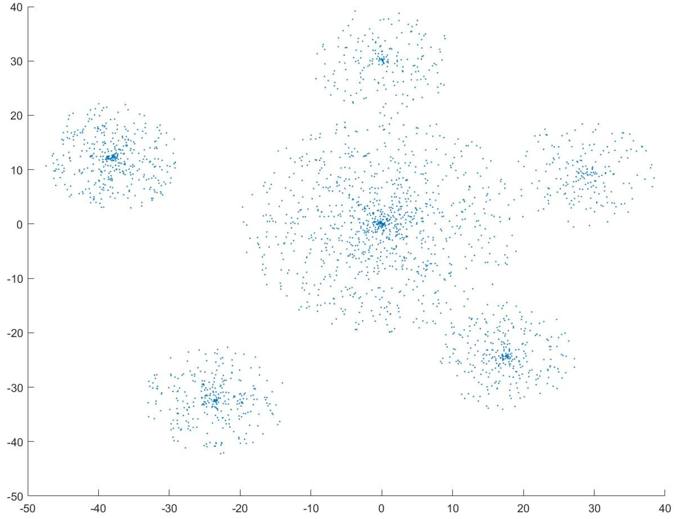
Figure 1 illustrates a sample distribution of city center points and employees, randomly generated for a case with 5 cities and 2000 employees. The radius of each city is determined in a way that city boundaries of neighboring cities will not overlap. The simulation scenarios, results, and analysis in Section 4.2 will be based on this model.
3.3.2. Parameters
As discussed earlier, once the traveling distance of employees is estimated, emission and fuel consumption factors are multiplied by the distance in our simulation study. Table 1 shows the emission factor and fuel consumption per kilometer used for different types of transportation in the experiment. Recall that we only allow a private vehicle traveling alone to maintain social distancing (single passenger). Note also that we take busses as a type of public transportation in estimation because not every city has a metro system in the region. The average number of passengers in different types of vehicles and grams of carbon emission per passenger per kilometer (g CO2/km/passenger) are based on the report by the European Environment Agency (EEA) [27]. The value of the parameter of public transit is smaller than that of private vehicle: g/km/passenger and g/km/passenger, respectively. Similarly, the amount of fuel consumption for different types of commuting is estimated based on the data from U.S. Department of Energy [28]. The average miles per gallon for private vehicle and transit bus are 24.2 mpg and 3.3 mpg, respectively. After converting these numbers into metrics, we obtain l/km/passenger and l/km/passenger, respectively.
In addition, we use a multiple in estimating regional infection rate for the experiment. This multiple is to compensate underreported cases. For instance, a group of researchers found out that the actual number of infections may be up to 12 times higher than reported [29]. In this experiment, we set the value of multiple as 10.
3.3.3. Scenarios
Different scenarios will be considered based on the regional infection rate of the cities, the number of neighboring cities, and the total number of employees allocated to the local satellite offices. For each scenario, the carbon emission, fuel consumption, and infection probabilities are estimated and compared with the baseline scenario without satellite offices. In each instance, the employees’ mode of travel is determined depending on the distance to the office, either in the core city or in neighboring cities. If the employees’ location is close enough to their assigned office, they can either walk or travel by bicycle. In our study, we set the distance for walking at 500 m and for a bicycle at 1 km. Otherwise, the employees’ mode of travel is randomly chosen between public transportation and the employee-owned vehicle, based on the rate of public transit, changing from 0% to 100%.
Measurement of infection risks is based on the risk probability of infected workers being found in the office. To investigate how it changes, different scenarios are considered on regional infection rate. The infection rate of both the core city and neighboring cities change from 1/10,000 to 2/10,000, while the same rate is applied for all neighboring cities. The expected number of employees at risk of infection is formulated as follows:
where is the total number of employees and is the risk measure at satellite office from Equation (12). This measure should be interpreted as the expected number of employees who may potentially be exposed to the virus at work. It is therefore expected that this number decreases significantly as the group size gets smaller in satellite offices. This way, it is possible to control risks of the business being temporarily suspended or closed, even after an office contracts the virus, which gives greater managerial advantages.
4. Experiment Results
A simulation model is developed via MATLAB, and experiments are conducted based on the instances created by the model. For each combination, 1000 different instances are randomly generated and three decision criteria are evaluated. To investigate different scenarios, we consider two cases: (1) one neighboring city and (2) multiple neighboring cities. In the first case, we focus on how regional infection rates of the two cities will impact the three decision criteria of carbon emission, fuel consumption, and infection risk at work. In the following case with multiple neighboring cities, we consider several scenarios to study the effect of the number of satellite offices opening in the neighboring cities on the decision criteria.
4.1. Single Neighboring City
In this experiment, we test the effect of opening a satellite office in a neighboring city when regional infection rates of the two cities may vary. Assuming that there is a core city and one neighboring city for it, a company’s decision will be either to open a satellite office in the neighboring city or not. In addition to the three decision criteria mentioned earlier, we further consider the expected number of employees exposed to infection at work, defined in Equation (15). Even if the infection probability in an office is higher, the total number of employees who might have close contact may not be larger if a smaller number of employees is allocated to the office, and hence the total number of employees that can be affected may also be small as a whole. Thus, this measure will be used as an indication of how serious the outbreak is at work, in comparison to the level of normal business operation.
Given that we consider a fixed number of employees (2000 in total), we change the number of the employees in each of the two cities. By changing the number of employees in both cities and the local infection probability in both cities, we consider the two scenarios. In scenario 1, the core city will be hit harder by the virus: the probability of infection for the neighboring city is fixed whereas the probability of the core city varies from 5 × 10⁻⁵ to 5 × 10⁻⁴ with an increment of 5 × 10⁻⁵. In scenario 2, on the other hand, the neighboring city will be hit harder: the probability of infection for the neighboring city is changed and the probability for the core city is fixed. These two scenarios are summarized in Table 2.
We begin with carbon emission and fuel consumption based on the number of employees in each city. In this experiment, we focus on the effect of the relative size of employees in the two cities on the distance-based criteria. The probability of taking public transportation is set to 50%. Not surprisingly, as more employees reside in the neighboring city, both measures increase sharply when there is no opening satellite office in the city. Since all employees are required to travel to the HQ in the core city no matter where they live, the average distance increases accordingly. On the other hand, when there is a satellite office put in place in the neighboring city, the average distance decreases and thereby the two criteria decrease as well. The amount of decrease is not as large, however, because the larger proportion of employees in the core city still travel to the HQ regardless. While the increasing/decreasing trend is linear for both criteria, the difference between the model with and without satellite office gets larger as more employees live in the neighboring city. The result is shown in Table 3.
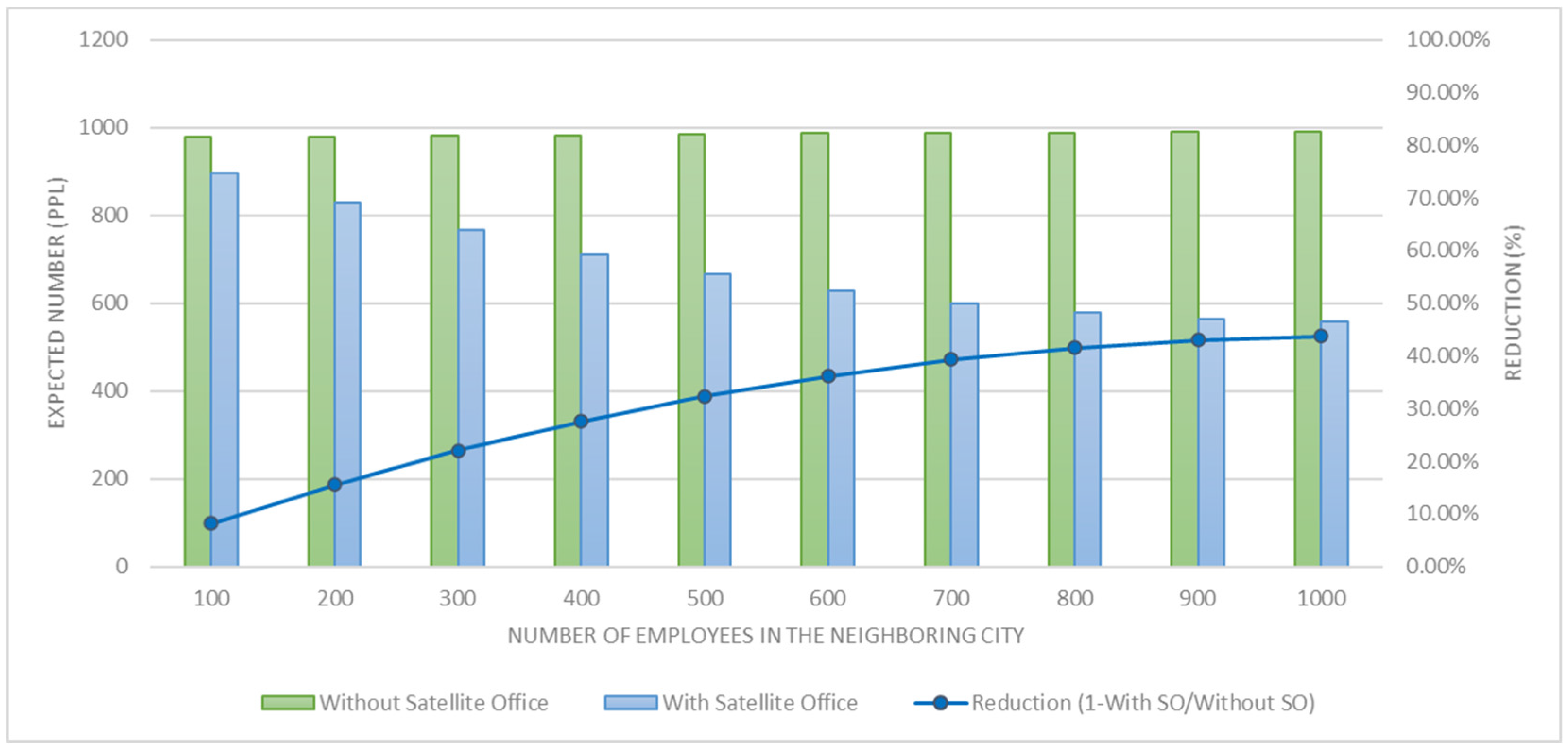
Table 4 shows the probability of infection occurrence at work when the infection probability in the city is set to 5 × 10⁻⁵. Note that the probability of infection of the HQ and the satellite office are defined in Equations (11) and (12), respectively. When there is no satellite office in the neighboring city, the probability of infection remains largely the same: only a limited amount increases as more employees may be infected while traveling longer distance to the HQ. With a satellite office opening in the neighboring city, however, the probability decreases significantly for the HQ as the number of employees working in the HQ decreases from 1900 to 1000. Conversely, the infection probability of the satellite office increases accordingly. It should be noted that the summation of the two probabilities always looks larger than that of the case without a satellite office. However, when it comes to the number of employees who may be potentially affected by the incident (such as self-quarantine and staying at home for 14 days), a clear indication of improvement can be observed. Assigning only 5% of the total employees (100 out of 2000) results in an 8.23% (from 997.59 to 897.17) reduction in the number, while the estimate increases sharply by 43.70% (from 991.33 to 558.12) when half of the employees are assigned to the different office (Reduction = 1 − (With SO / Without SO)). This result shows that the opening of the satellite office can mitigate the impact of being exposed to the virus for the business. As the number of employees living in the neighboring city increases, the benefit of having the satellite office becomes greater. The comparison of the expected number of employees exposed to the virus at work for the case without a satellite office and the case with a satellite office is shown in Figure 2.
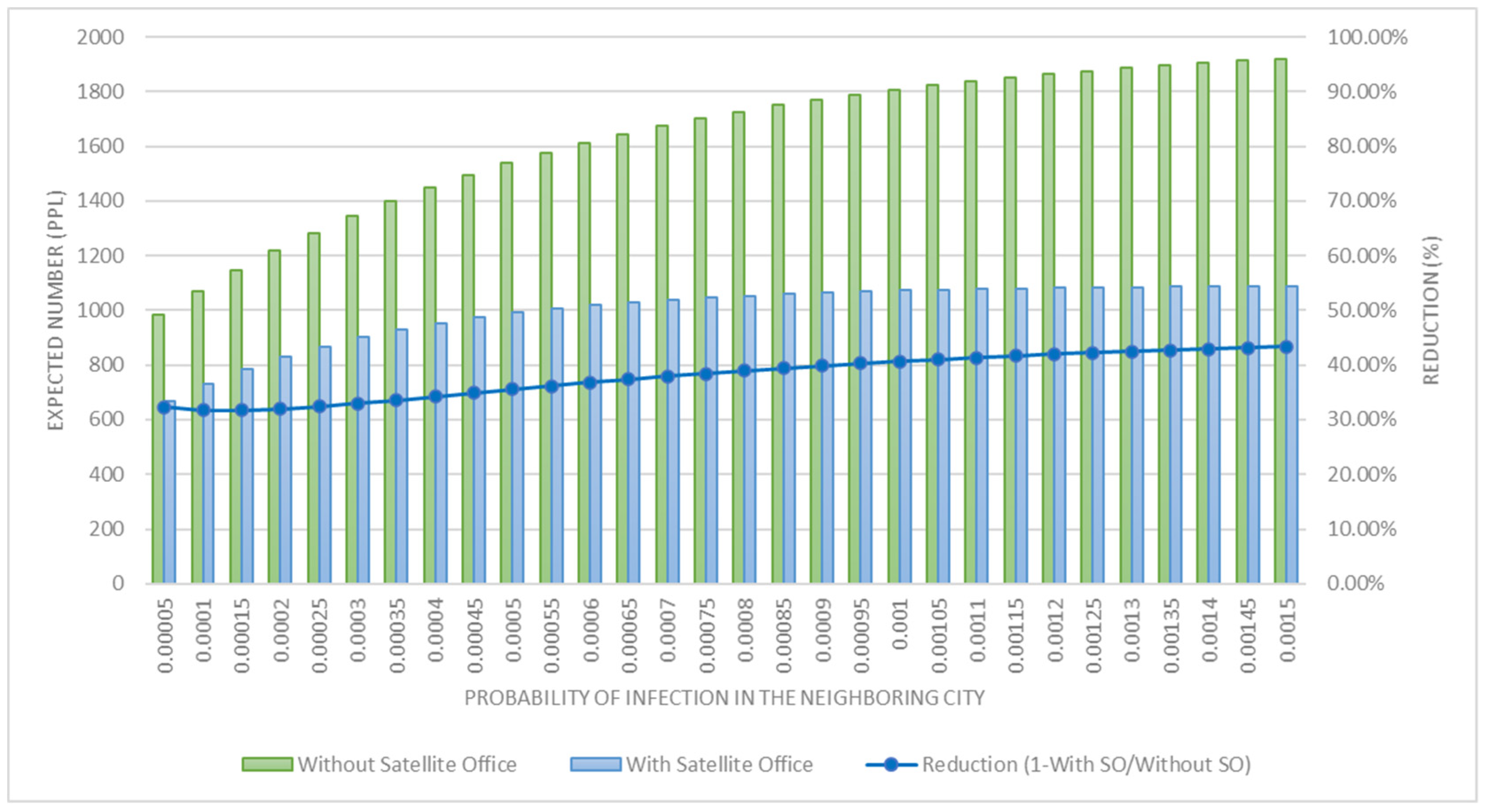
Then, the effect of the probability of infection of the core city to the expected number of employees exposed to the virus at work is analyzed. The results are shown in Table 5 and Figure 3. As the infection probability of the core city increases, the expected number of employees exposed to the virus at work increases in both cases: with a satellite office and without a satellite office. However, the expected number in the case without a satellite office outnumbered the case with a satellite office. The ratio between the two cases (with satellite office/without satellite office) increases as the infection probability increases; however, it is all below 80%.
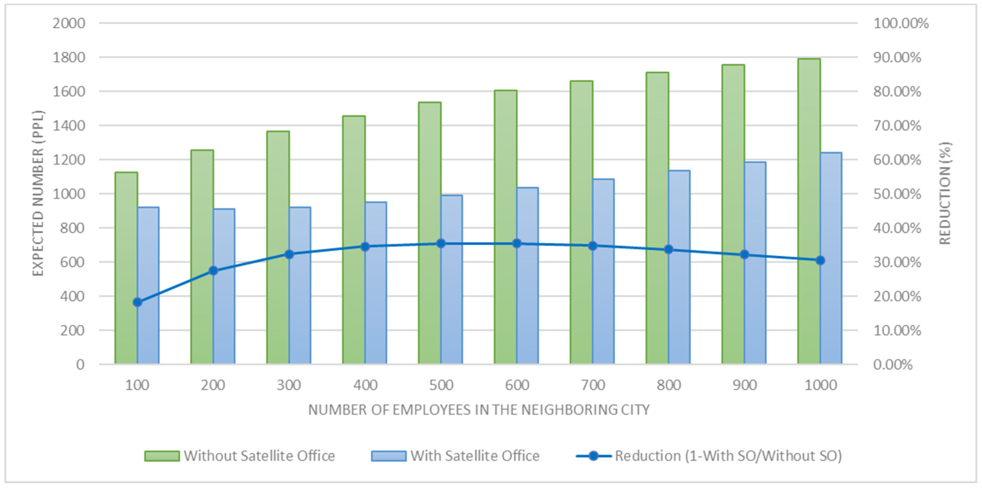
Then we check scenario 2, where the infection probability of the neighboring city increases whereas that of the core city is fixed to 5 × 10⁻⁵. In scenario 2, the situation of the virus in the neighboring city is worse than the core city and we check whether it is still beneficial to open the satellite office in such a case. Similar to scenario 1, we analyzed the effect of the probability of infection of the neighboring city to the expected number of employees exposed to the virus. When the probability of infection of the neighboring city is much higher than that of the core city, the expected number of employees exposed to the virus in the case with a satellite office and in the case without a satellite office is checked. Different to scenario 1, as the number of employees in the neighboring city increases, the expected number of employees exposed also increases in the case with a satellite office. The ratio between the two cases (with satellite office/without satellite office) has a U-shaped pattern as it decreases in the beginning and then increases after the number of employees in the neighboring city passes 500. However, the fact that the expected number in the case with a satellite office is less than the one in the case without a satellite office is still the same for both scenarios. The results are shown in Figure 4.
We fix the number of employees residing in the core city and the neighboring city to 1500 and 500, correspondingly, then check the relationships between the expected number of employees exposed and the infection probability of the neighboring city. The expected number increases as the probability of the infection of the neighboring city increases in both cases. However, the case without a satellite office is higher sloped than the case with a satellite office. This is because, in the case with the satellite office, the number of employees who can be infected is limited to 500; however, in the case without the satellite office, 2000 employees all commute to the HQ and therefore the number of employees who can be infected can keep increasing until it reaches 2000. The same pattern is found in all combinations of the number of employees in each city. The result is shown in Figure 5.
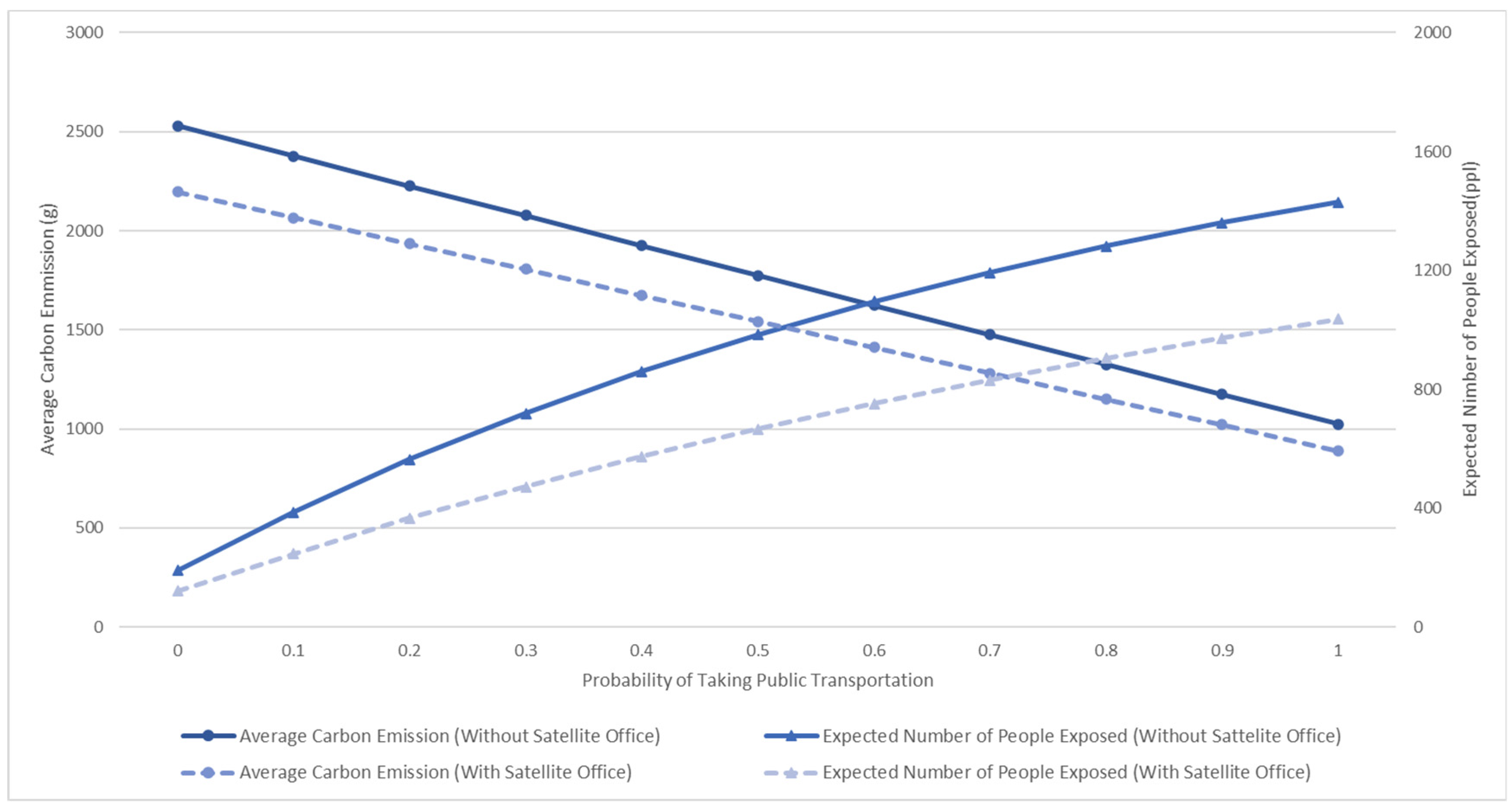
Lastly, we check the impact of public transportation. The two criteria, carbon emission and the expected number of people exposed to the virus are checked as we increase the probability of choosing public transportation instead of a private vehicle. As we expected, the average carbon emission decreases when more people decide to take a public transportation as it is the less carbon generating mode of transportation per km per people. Similar to the previous tests, when the satellite office is opened, the amount of emission decreases. This is because opening the satellite office decreases the distance of traveling by allowing the employees to commute to a closer office. Different from carbon emission, the expected number of people exposed to the virus increases as the chance of taking public transportation increases. This is because taking public transportation is riskier in terms of infection as the chance of contact to any possible infected person gets higher. The results are shown in Figure 6.
4.2. Multiple Neighboring Cities
In this chapter, five neighboring cities that are identical in terms of the number of employees and regional infection probabilities are considered as potential candidates for satellite offices. Given the total number of employees as 2000, 1000 of them reside in the core city, and the remaining 1000 live in the five neighboring cities (200 each). In this experiment, the same decision criteria are evaluated based on the proportion of employees who determine to travel using public transportation and the number of satellite offices opening in the neighboring cities. In the same way as before, we compare two different cases of with and without satellite office in terms of carbon emission, fuel consumption, the probability of infection occurrence in the office, and the expected number of employees exposed to the virus at work. Note that the probability of regional infection of each city is set to 5 × 10⁻⁵. The result of the simulation is summarized in Figure 7.
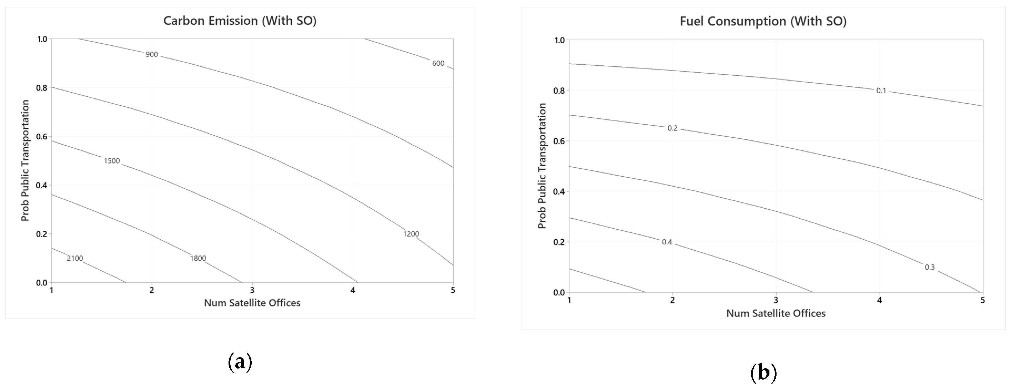
Figure 7a shows the results of the simulation on the amount of carbon emission with respect to the number of satellite offices and the percentage of workers who use public transportation. Opening more satellite offices in the neighboring cities leads to a decrease in average traveling distance, as well as in the amount of carbon emission. When more employees decide to take public transportation instead of using their own vehicle, the average amount of carbon emission decreases significantly as the emission factor for public transportation is a lot lower than that for a private vehicle. Likewise, Figure 7b shows the results of the simulation on the amount of fuel consumption with respect to the number of satellite offices and the percentage of workers who use public transportation. Opening more satellite offices in the neighboring cities results in the reduction of fuel consumption. When more employees decide to take public transportation instead of using their own vehicle, the average amount of fuel consumption increases significantly as the emission factor for public transportation is a lot higher than that for a private vehicle.
Table 6 and Table 7 summarize the reduction in carbon emission and fuel consumption over all different proportions of employees using public transportation. The rate of reduction is stable across all regions when the company locates a new satellite office: approximately a 10.18% reduction is expected when there is one satellite office. Similarly, 20.35%, 30.54%, 40.72%, and 50.89% reductions are observed when there are 2, 3, 4, and 5 satellite offices across the region, respectively.
5. Discussion
The results suggest important managerial implications in making decisions related to satellite offices. First, as shown in the single-neighboring city case, when the infection probability of the two cities are the same, one can expect greater reduction in the number of employees exposed to the virus at work by opening a satellite office and allocating employees to the site. This is rather straightforward because the reduction in commuting distance leads to less carbon emission and fuel consumption, and the infection probability decreases as office capacity reduces as well. When the infection rate of the neighboring city is higher, however, it may not be clear as to whether opening a satellite office in the neighboring city is still beneficial. Based on our model, however, it is still the case because there is a significant amount of reduction in terms of the expected number of employees exposed as well as carbon emission and fuel consumption.
It should be noted that cost information was not incorporated into our framework. For instance, we did not consider the fixed, operating, and shutdown costs of satellite offices. The social and environmental costs of carbon emission were not considered either. Therefore, careful examination is needed when interpreting the simulation results presented in this study. Since we did not consider the fixed and operating costs of satellite offices, it might be worse off to open new satellite offices, depending on the actual costs of the company. The decision may also be influenced by the target infection probability at work set by the company. They may be willing to embrace higher operating costs of opening multiple offices if their estimated shutdown cost is significantly higher. Therefore, to make the final conclusion on opening satellite offices, companies should incorporate all of their costs and benefits thoroughly.
Once measures to sufficiently compare the costs and benefits of opening satellite offices are developed, one can use its own cost estimates with our model to derive the optimal satellite office locations and allocations of their own. For instance, a full optimization model can be developed so as to provide a fair comparison among all of the criteria and finally incorporate the costs and benefits quantitatively. The decision criteria discussed in our model can be extended to build a mathematical programming model. Given the target carbon emission and infection probability in the office, a company can explore the optimal satellite office setup possible. The solution in turn gives the optimal allocation of employees to minimize the total operating costs of the company, while keeping the infection probability less than the target number.
Lastly, even though there is no sufficient cost information that allows us to compare the benefits and costs together, companies can still obtain valuable business insights from our research. Contingency plans for the office setup in the case of a pandemic can also be designed to mitigate business risks.
6. Conclusions
In this research, we investigated the effectiveness of operating satellite offices as a tool for business sustainability. Since the environmental impact of a business is regarded as one of the pressing issues in academia and industry, we incorporated environmental factors such as carbon emission and fuel consumption. In addition, with the arrival of the COVID-19 pandemic, the landscape of the work environment has changed drastically. The possibility of infection in the office has become a very important issue, and this changes how people work. Taking this shift in office environment into account, we developed a new measure indicating the probability of whether an employee is infected by the virus. If there is anyone infected in the office, the company has to shut down the whole office or at least some part of it and then sanitize the area where that person came in contact with. Because of these events, quite a number of employees have to be relocated and quarantined, therefore decreasing productivity. Hence, we developed another measure that can induce the cost afterwards, and measure the expected number of employees exposed to the virus at work.
In order to model these two very different objectives, we considered a simulation study to find the results of opening and operating a satellite office based on different scenarios. We checked the relationships of the four measures, the infection probability, portion of employees in terms of their cities of residence, the number of satellite offices opened, etc.
To scrutinize the impact of satellite offices, we first considered a simple single-neighboring city case where there is one core city and one neighboring city. In the multiple-neighboring cities case, the company can decide how many additional satellite offices should be opened. In both experiments, the benefits of opening a new satellite office are significant. In all decision criteria, a significant amount of reduction is observed by allocating employees to their designated satellite offices. Both the amount of carbon emission and fuel consumption decreased for all cases. More importantly, the probability of infection at work can also be evaluated. Given the capacity of the office, we can calculate the probability of infection occurrence there. This probability indicates the possibility of having at least one infected worker at the office. Since this leads to business disruption and employee health concerns, a company should be able to manage the risk. By adopting satellite offices in business operation and distributing employees to different locations, risks can be significantly reduced.
As discussed earlier, the model considered in this research focused on each criterion separately. To make the final decision on whether or not to open the satellite office, related costs have to be reconsidered. Future research should conduct a cost and benefit analysis and should develop a full optimization model that can provide a fair comparison among all of the criteria and finally incorporate the costs and benefits quantitatively.
Author Contributions
Conceptualization, S.K, Y.L. and B.C.; methodology, S.K and Y.L.; validation, B.C.; formal analysis, S.K. and Y.L.; investigation, S.K, Y.L. and B.C.; simulation, S.K.; writing—original draft preparation, S.K. and Y.L.; writing—review and editing, B.C.; visualization, S.K. and Y.L.; project administration, Y.L.; funding acquisition, Y.L. All authors have read and agreed to the published version of the manuscript.
Funding
Seungbeom Kim’s work was supported by 2020 Hongik University Research Fund. Byungchul Choi’s work was supported by the Hankuk University of Foreign Studies Research Fund of 2021.
Institutional Review Board Statement
Not applicable.
Informed Consent Statement
Not applicable.
Data Availability Statement
The data are self-generated by the computer simulation.
Conflicts of Interest
The authors declare no conflict of interest.
References
- Brynjolfsson, E.; Horton, J.; Ozimek, A.; Rock, D.; Sharma, G.; TuYe, H.-Y. COVID-19 and Remote Work: An Early Look at US Data; NEBR Working Paper No. 27344; National Bureau of Economic Research: Cambridge, MA, USA, 2020. [Google Scholar]
- Olson, M.H. Remote office work: Changing work patterns in space and time. Commun. ACM 1983, 26, 182–187. [Google Scholar] [CrossRef]
- Fritz, M.E.W.; Higa, K.; Narasimhan, S. Telework: Exploring the borderless office. In Proceedings of the Twenty-Seventh Hawaii International Conference on System Sciences HICSS, Wailea, HI, USA, 4–7 January 1994; pp. 149–158. [Google Scholar]
- Rao, V.S. The implementation of satellite offices: Initial recommendations based on observations from one site. In Proceedings of the Twenty-Eighth Annual Hawaii International Conference on System Sciences, Wailea, HI, USA, 3–6 January 1995; Volume 4, pp. 426–435. [Google Scholar]
- Belzunegui-Eraso, A.; Erro-Garcés, A. Teleworking in the Context of the Covid-19 Crisis. Sustainability 2020, 12, 3662. [Google Scholar] [CrossRef]
- CDC. Communities, Schools, Workplaces, & Events. Centers for Disease Control and Prevention, 2020. Available online: https://www.cdc.gov/coronavirus/2019-ncov/community/office-buildings.html (accessed on 26 November 2020).
- CDC. Health Departments. Centers for Disease Control and Prevention, 2020. Available online: https://www.cdc.gov/coronavirus/2019-ncov/php/contact-tracing/contact-tracing-plan/contact-tracing.html (accessed on 29 May 2021).
- Nawaz, W.; Koç, M. Exploring Organizational Sustainability: Themes, Functional Areas, and Best Practices. Sustainability 2019, 11, 4307. [Google Scholar] [CrossRef] [Green Version]
- Morganson, V.J.; Major, D.A.; Oborn, K.L.; Verive, J.M.; Heelan, M.P. Comparing telework locations and traditional work arrangements. J. Manag. Psychol. 2010, 25, 578–595. [Google Scholar] [CrossRef]
- Qvortrup, L. From Teleworking to Networking. In Teleworking: International Perspectives; Routledge: London, UK, 1998; pp. 21–39. [Google Scholar]
- Garrett, R.K.; Danziger, J.N. Which telework? Defining and testing a taxonomy of technology-mediated work at a distance. Soc. Sci. Comput. Rev. 2007, 25, 27–47. [Google Scholar] [CrossRef] [Green Version]
- Baruch, Y. Teleworking: Benefits and pitfalls as perceived by professionals and managers. New Technol. Work. Employ. 2000, 15, 34–49. [Google Scholar] [CrossRef]
- Baruch, Y.; Nicholson, N. Home, Sweet Work: Requirements for Effective Home Working. J. Gen. Manag. 1997, 23, 15–30. [Google Scholar] [CrossRef]
- Dima, A.-M.; Țuclea, C.-E.; Vrânceanu, D.-M.; Țigu, G. Sustainable Social and Individual Implications of Telework: A New Insight into the Romanian Labor Market. Sustainability 2019, 11, 3506. [Google Scholar] [CrossRef] [Green Version]
- Haar, J.M.; Russo, M.; Sunyer, A.; Ollier-Malaterre, A. Outcomes of work–life balance on job satisfaction, life satisfaction and mental health: A study across seven cultures. J. Vocat. Behav. 2014, 85, 361–373. [Google Scholar] [CrossRef]
- Boiral, O.; Brotherton, M.-C.; Rivaud, L.; Guillaumie, L. Organizations’ Management of the COVID-19 Pandemic: A Scoping Review of Business Articles. Sustainability 2021, 13, 3993. [Google Scholar] [CrossRef]
- Cooper, L. Location-Allocation Problems. Oper. Res. 1963, 11, 331–343. [Google Scholar] [CrossRef]
- Arabani, A.B.; Farahani, R.Z. Facility location dynamics: An overview of classifications and applications. Comput. Ind. Eng. 2012, 62, 408–420. [Google Scholar] [CrossRef]
- Cachon, G.P. Retail Store Density and the Cost of Greenhouse Gas Emissions. Manag. Sci. 2014, 60, 1907–1925. [Google Scholar] [CrossRef] [Green Version]
- Chaabane, A.; Ramudhin, A.; Paquet, M. Design of sustainable supply chains under the emission trading scheme. Int. J. Prod. Econ. 2012, 135, 37–49. [Google Scholar] [CrossRef]
- Turken, N.; Carrillo, J.; Verter, V. Facility location and capacity acquisition under carbon tax and emissions limits: To centralize or to decentralize? Int. J. Prod. Econ. 2017, 187, 126–141. [Google Scholar] [CrossRef]
- Chen, L.; Olhager, J.; Tang, O. Manufacturing facility location and sustainability: A literature review and research agenda. Int. J. Prod. Econ. 2014, 149, 154–163. [Google Scholar] [CrossRef] [Green Version]
- COVID-19 Event Risk Assessment Planning Tool. Available online: https://covid19risk.biosci.gatech.edu/ (accessed on 24 February 2021).
- Das, S.K.; Roy, S.K. Effect of variable carbon emission in a multi-objective transportation-p-facility location problem under neutrosophic environment. Comput. Ind. Eng. 2019, 132, 311–324. [Google Scholar] [CrossRef]
- Jia, H.; Xu, Y.; Tian, G.; Zhou, M.C.; Zhang, J.; Zhang, H. Random Energy-efficient Models for Sustainable Facility Location Subject to Carbon Emission, Economical, Capacitated and Regional Constraints. IEEE Access 2018, 6, 72757–72765. [Google Scholar] [CrossRef]
- Schwartz, S. Public Transit and COVID-19 Pandemic: Global Research and Best Practices. American Public Transportation Association, 2020. Available online: https://www.apta.com/researchtechnical-resources/research-reports/public-transit-and-covid-19-pandemic-globalresearch-and-best-practices (accessed on 26 November 2020).
- CO2 Emissions from Passenger Transport—European Environment Agency. Available online: https://www.eea.europa.eu/media/infographics/co2-emissions-from-passenger-transport/view (accessed on 22 February 2021).
- Alternative Fuels Data Center: Public Transportation. Available online: https://afdc.energy.gov/conserve/mass_transit.html (accessed on 22 February 2021).
- Rahmandad, H.; Lim, T.Y.; Sterman, J. Estimating the global spread of COVID-19. MedRxiv 2020. [Google Scholar] [CrossRef]
Figure 1.
Locations of each employee living in the core city and the five neighboring cities are generated by the simulation. The distance and angle between the centers of five cities and the origin is decided based on the two vectors and . The coordinate of the location of each employee is generated based on the vectors , , , and , which are the number of employees in each city, the radius of each city, the random distance of the location of the employee from the center of the city, and the random angle of the location of the employee from the center of the city, respectively.

Figure 2.
Expected number of employees exposed to the virus at work based on the number of employees in the neighboring city (infection probability in both cities is set to 5 × 10⁻⁵).
Figure 2.
Expected number of employees exposed to the virus at work based on the number of employees in the neighboring city (infection probability in both cities is set to 5 × 10⁻⁵).

Figure 3.
Expected number of exposed to the virus at work based on the infection probability in the core city.
Figure 3.
Expected number of exposed to the virus at work based on the infection probability in the core city.

Figure 4.
Expected number of exposed to the virus at work based on the number of employees in the neighboring city (infection probabilities in the core city and the neighboring city are set to 5 × 10⁻⁵ and 5 × 10⁻⁴, correspondingly).
Figure 4.
Expected number of exposed to the virus at work based on the number of employees in the neighboring city (infection probabilities in the core city and the neighboring city are set to 5 × 10⁻⁵ and 5 × 10⁻⁴, correspondingly).

Figure 5.
Expected number of employees exposed to the virus at work based on the infection probability of the neighboring city.
Figure 5.
Expected number of employees exposed to the virus at work based on the infection probability of the neighboring city.

Figure 6.
Average carbon emission and expected number of employees exposed to the virus at work based on the probability of taking public transportation.
Figure 6.
Average carbon emission and expected number of employees exposed to the virus at work based on the probability of taking public transportation.

Figure 7.
Contour graphs of: (a) Carbon emission versus number of satellite offices and probability of employees to take public transportation; (b) Fuel consumption versus number of satellite offices and probability of employees to take public transportation.
Figure 7.
Contour graphs of: (a) Carbon emission versus number of satellite offices and probability of employees to take public transportation; (b) Fuel consumption versus number of satellite offices and probability of employees to take public transportation.


Table 1.
Average number of passengers, emission factor, and estimated fuel consumption by types of commuting.
Table 1.
Average number of passengers, emission factor, and estimated fuel consumption by types of commuting.
| Type of Commute | Number of Passengers | Emission Factor (CO2 g/km/passenger) 1 | Fuel Consumption (l/km/passenger) 2 |
|---|---|---|---|
| Walk or bicycle | 1 | 0 | 0 |
| Public transportation | 9.1 2 | 68 | 0.0783 |
| Private vehicle | 1 | 158 | 0.0971 |
Source: 1 European Environment Agency 2 U.S. Department of Energy.
Table 2.
One neighboring city (Total number of employees is set to 2000).
| Scenarios | Number of Employees Allocated to the Satellite Office | Probability of Infection | |
|---|---|---|---|
| Core City | Neighboring City | ||
| 1 | 100–1000 | 5 × 10⁻⁵–5 × 10⁻⁴ | 5 × 10⁻⁵ |
| 2 | 100–1000 | 5 × 10⁻⁵ | 5 × 10⁻⁵–5 × 10⁻⁴ |
Table 3.
Average carbon emission and average fuel consumption.
| Number of Employees | Traveling Distance (km) | Carbon Emission (g) | Fuel Consumption (l) | ||||
|---|---|---|---|---|---|---|---|
| Core City | Neighboring City | Without SO | With SO | Without SO | With SO | Without SO | With SO |
| 1900 | 100 | 11.01 | 9.75 | 1241.90 | 1098.48 | 0.6809 | 0.6026 |
| 1800 | 200 | 12.03 | 9.50 | 1357.08 | 1070.73 | 0.7441 | 0.5872 |
| 1700 | 300 | 13.04 | 9.25 | 1470.70 | 1041.46 | 0.8065 | 0.5711 |
| 1600 | 400 | 14.05 | 8.99 | 1585.99 | 1013.03 | 0.8690 | 0.5553 |
| 1500 | 500 | 15.07 | 8.75 | 1700.90 | 985.58 | 0.9320 | 0.5397 |
| 1400 | 600 | 16.08 | 8.50 | 1815.89 | 956.40 | 0.9949 | 0.5245 |
| 1300 | 700 | 17.10 | 8.25 | 1929.75 | 928.14 | 1.0587 | 0.5093 |
| 1200 | 800 | 18.11 | 8.00 | 2045.50 | 900.39 | 1.1211 | 0.4936 |
| 1100 | 900 | 19.12 | 7.75 | 2158.42 | 871.06 | 1.1842 | 0.4779 |
| 1000 | 1000 | 20.14 | 7.50 | 2274.00 | 843.48 | 1.2471 | 0.4622 |
Table 4.
Probability of the occurrence of infection and the expected number of employees exposed to the virus at work (infection probability in both cities is set to 5 × 10⁻⁵).
Table 4.
Probability of the occurrence of infection and the expected number of employees exposed to the virus at work (infection probability in both cities is set to 5 × 10⁻⁵).
| Number of Employees | Probability of the Occurrence of the Infection | Expected Number of Employees Exposed to the Virus at Work | ||||||
|---|---|---|---|---|---|---|---|---|
| Core City | Neighboring City | Without SO | With Satellite Office | Without SO | With SO | Reduction | ||
| HQ | HQ | SO | Sum | |||||
| 1900 | 100 | 0.4888 | 0.4705 | 0.0315 | 0.5021 | 977.59 | 897.17 | 8.23% |
| 1800 | 200 | 0.4900 | 0.4529 | 0.0621 | 0.5150 | 979.97 | 827.64 | 15.54% |
| 1700 | 300 | 0.4906 | 0.4341 | 0.0917 | 0.5258 | 981.23 | 765.48 | 21.99% |
| 1600 | 400 | 0.4914 | 0.4151 | 0.1200 | 0.5350 | 982.81 | 712.09 | 27.55% |
| 1500 | 500 | 0.4923 | 0.3951 | 0.1479 | 0.5430 | 984.65 | 666.64 | 32.30% |
| 1400 | 600 | 0.4931 | 0.3748 | 0.1747 | 0.5494 | 986.24 | 629.49 | 36.17% |
| 1300 | 700 | 0.4935 | 0.3531 | 0.2004 | 0.5535 | 986.95 | 599.29 | 39.28% |
| 1200 | 800 | 0.4941 | 0.3308 | 0.2257 | 0.5565 | 988.27 | 577.56 | 41.56% |
| 1100 | 900 | 0.4952 | 0.3082 | 0.2503 | 0.5585 | 990.42 | 564.34 | 43.02% |
| 1000 | 1000 | 0.4957 | 0.2846 | 0.2735 | 0.5581 | 991.33 | 558.12 | 43.70% |
Table 5.
The effect of the infection probability of the core city to the expected number of employees exposed to the virus at work in scenario 1 (the number of employees in the core city and the neighboring city is 1500 and 500, correspondingly. the infection probability in the neighboring city is 5 × 10⁻⁵).
| Infection Probability of the Core City | Probability of the Occurrence of the Infection | Expected Number of Employees Exposed to the Virus at Work | |||
|---|---|---|---|---|---|
| HQ Only | With Satellite Office | HQ Only | With SO | ||
| HQ | HQ | SO | |||
| 5 × 10⁻⁵ | 0.4923 | 0.3951 | 0.1479 | 977.59 | 897.17 |
| 10−4 | 0.7184 | 0.6340 | 0.1476 | 979.97 | 827.64 |
| 1.5 × 10⁻⁴ | 0.8437 | 0.7782 | 0.1480 | 981.23 | 765.48 |
| 2 × 10⁻⁴ | 0.9135 | 0.8660 | 0.1479 | 982.81 | 712.09 |
| 2.5 × 10⁻⁴ | 0.9519 | 0.9187 | 0.1479 | 984.65 | 666.64 |
| 3 × 10⁻⁴ | 0.9735 | 0.9510 | 0.1481 | 986.24 | 629.49 |
| 3.5 × 10⁻⁴ | 0.9852 | 0.9703 | 0.1474 | 986.95 | 599.29 |
| 4 × 10⁻⁴ | 0.9918 | 0.9821 | 0.1478 | 988.27 | 577.56 |
| 4.5 × 10⁻⁴ | 0.9954 | 0.9891 | 0.1478 | 990.42 | 564.34 |
| 5 × 10⁻⁴ | 0.9975 | 0.9934 | 0.1480 | 991.33 | 558.12 |
Table 6.
Reduction in carbon emission.
| Proportion of Employees Using Public Transportation | Number of Satellite Offices | |||||
|---|---|---|---|---|---|---|
| 0 | 1 | 2 | 3 | 4 | 5 | |
| 0.0 | 2551.90 | 2291.98 | 2033.38 | 1773.47 | 1513.91 | 1253.66 |
| 0.1 | 2401.49 | 2156.91 | 1912.30 | 1667.36 | 1421.82 | 1178.49 |
| 0.2 | 2248.54 | 2019.83 | 1792.94 | 1563.00 | 1333.52 | 1104.03 |
| 0.3 | 2096.02 | 1882.87 | 1669.36 | 1456.86 | 1242.86 | 1029.62 |
| 0.4 | 1945.57 | 1747.48 | 1548.47 | 1351.19 | 1154.08 | 955.02 |
| 0.5 | 1792.72 | 1610.09 | 1426.90 | 1246.87 | 1062.93 | 879.43 |
| 0.6 | 1641.97 | 1474.70 | 1308.44 | 1139.89 | 972.54 | 805.38 |
| 0.7 | 1489.55 | 1338.19 | 1186.25 | 1034.25 | 882.99 | 731.80 |
| 0.8 | 1338.48 | 1202.12 | 1065.36 | 928.62 | 793.20 | 657.19 |
| 0.9 | 1185.47 | 1064.49 | 943.67 | 823.41 | 703.20 | 582.40 |
| 1.0 | 1033.64 | 928.36 | 823.30 | 717.78 | 612.37 | 507.28 |
Table 7.
Reduction in fuel consumption.
| Proportion of Employees Using Public Transportation | Number of Satellite Offices | |||||
|---|---|---|---|---|---|---|
| 0 | 1 | 2 | 3 | 4 | 5 | |
| 0.0 | 0.6076 | 0.5457 | 0.4841 | 0.4223 | 0.3605 | 0.2985 |
| 0.1 | 0.5531 | 0.4968 | 0.4404 | 0.3840 | 0.3274 | 0.2714 |
| 0.2 | 0.4979 | 0.4473 | 0.3972 | 0.3463 | 0.2954 | 0.2445 |
| 0.3 | 0.4430 | 0.3980 | 0.3528 | 0.3079 | 0.2627 | 0.2176 |
| 0.4 | 0.3886 | 0.3490 | 0.3092 | 0.2698 | 0.2305 | 0.1907 |
| 0.5 | 0.3334 | 0.2994 | 0.2654 | 0.2320 | 0.1977 | 0.1634 |
| 0.6 | 0.2790 | 0.2505 | 0.2224 | 0.1935 | 0.1651 | 0.1367 |
| 0.7 | 0.2239 | 0.2012 | 0.1783 | 0.1554 | 0.1328 | 0.1101 |
| 0.8 | 0.1693 | 0.1521 | 0.1346 | 0.1174 | 0.1003 | 0.0830 |
| 0.9 | 0.1141 | 0.1025 | 0.0908 | 0.0793 | 0.0678 | 0.0561 |
| 1.0 | 0.0593 | 0.0532 | 0.0472 | 0.0412 | 0.0351 | 0.0291 |
Publisher’s Note: MDPI stays neutral with regard to jurisdictional claims in published maps and institutional affiliations. |
© 2021 by the authors. Licensee MDPI, Basel, Switzerland. This article is an open access article distributed under the terms and conditions of the Creative Commons Attribution (CC BY) license (https://creativecommons.org/licenses/by/4.0/).
Share and Cite
MDPI and ACS Style
Kim, S.; Lee, Y.; Choi, B. Adoption of Satellite Offices in Response to a Pandemic: Sustainability and Infection Control. Sustainability 2021, 13, 8008. https://doi.org/10.3390/su13148008
AMA Style
Kim S, Lee Y, Choi B. Adoption of Satellite Offices in Response to a Pandemic: Sustainability and Infection Control. Sustainability. 2021; 13(14):8008. https://doi.org/10.3390/su13148008
Chicago/Turabian StyleKim, Seungbeom, Yooneun Lee, and Byungchul Choi. 2021. "Adoption of Satellite Offices in Response to a Pandemic: Sustainability and Infection Control" Sustainability 13, no. 14: 8008. https://doi.org/10.3390/su13148008
Note that from the first issue of 2016, this journal uses article numbers instead of page numbers. See further details here.