Changes in a Bottom-Up Vehicular Emissions Inventory and Its Impact on Air Pollution During COVID-19 Lockdown in São Paulo, Brazil
 Sergio Ibarra-Espinosa1,2,3*
  Amanda Rehbein4
  Edmilson Dias de Freitas4
  Leila Martins5
  Maria de Fatima Andrade4
  Eduardo Landulfo1
- 1Laboratorio de Aplicações Ambientais de Lasers, Instituto de Pesquisas Energéticas e Nucleares, São Paulo, Brazil
- 2Cooperative Institute for Research in Environmental Sciences, University of Colorado-Boulder, Boulder, CO, United States
- 3Global Monitoring Laboratory, National Oceanic and Atmospheric Administration (NOAA), Boulder, CO, United States
- 4Departamento de Ciências Atmosféricas, Universidade de São Paulo, São Paulo, Brazil
- 5Departament of Chemistry, Federal University of Technology, Londrina, Brazil
Due to coronavirus disease 2019 (COVID-19), many cities implemented strict lockdown to stop the spread of this new disease. Consequently, it was reported lower levels of air pollution due to less human activity outdoors. The changes were registered using surface monitoring stations or satellite observations. However, modeling those environmental changes has remained a challenge because of our limitations in the emissions estimation and also, for the numerical modeling itself. In this study, the vehicular emissions were estimated for March 2020 in the megacity of São Paulo using the Vehicular Emissions INventory model (VEIN). The emissions estimation showed an increment of VOC/NO2 downtown, due to the decrease in circulation of urban transportation and light vehicles. Then, a set of Weather Research and Forecasting models with chemistry (WRF-Chem) simulations were performed with different chemical mechanisms and initial conditions. The modeled diurnal cycles represent the variations observed in March 2020 for the periods pre-lockdown, transition, and lockdown. However, it is imperative to include other sources than vehicular to have a local and comprehensive emissions inventory.
Introduction
The world has been under an unprecedented global health crisis due to the Coronavirus disease (COVID-19) Pandemic. To date, there are more than 360 million and 5.5 million registered COVID-19 cases and deaths, respectively, across the world (Dong et al., 2020). COVID-19 originated in the Chinese city of Wuhan and was officially reported on 30 December 2019 (Infectious Diseases, 2019). This disease proved to be deadly to vulnerable groups with rapid spread (Chan et al., 2020; Wang et al., 2020). Therefore, governments across the world started to impose strict lockdowns to avoid the spread of COVID-19 (Hamzelou, 2020). Lockdown measures, despite being called “war tactics” to impose families of whole countries to stay at home, with all the related economical costs and changes in our normal way of live (Hamzelou, 2020; Biroli et al., 2021), have shown to be effective to control COVID-19 (Alfano and Ercolano, 2020). For instance, Ibarra-Espinosa et al. (2022a) found that increasing the isolation by 5% would avoid 438 cases and 21 deaths per day in São Paulo, Brazil.
There is evidence that lesser human activities reduce levels of air pollution. In a global analysis, it was found reductions up to –70% for nitrogen dioxide NO2, between –30 and –40% for fine particulate matter of PM2.5 (Sokhi et al., 2021). Bao and Zhang (2020) found that human mobility was reduced by about –70 and the air pollutants PM2.5, NO2, and CO were reduced by –5.93, –24.7, and –4.6%, respectively, similar to other observational studies (Venter et al., 2020; Barua and Nath, 2021). Nevertheless, it was discovered that the secondary pollutant O3 presented increments because of lockdown. For instance, O3 increased by 40% in Mexico city (Hernandez-Paniagua et al., 2021) and by 30% in European cities (Grange et al., 2021). However, the transport of air masses and air pollution have a significant impact on local air pollution and this aspect must be considered when studying air pollution. In this sense, Thunis et al. (2021) identified that in Europe, the local emissions impact mostly the city center, while other areas are largely impacted by the transport of pollution originating in other cities. In the US, Li et al. (2015) found that the city of Phoenix in the state of Arizona is frequently impacted by the air pollution originating in California.
During the current COVID-19 crisis, Internet companies such as Google, Apple, and TomTom started releasing public and anonymized data about daily changes in mobility in cities across the world and changes with basis on pre-lockdown periods (Apple, 2022; Google, 2022). Then, these data have been used as a proxy to represent the emissions changes. Hence, Guevara et al. (2021) presented an emission inventory for Europe with factors derived from mobility datasets, finding reductions of 33% for nitrogen oxides (NOX), 8% for volatile organic compounds (VOC), 7% and sulfur oxides (SOX). Their study showed that the transport sector presented stronger reductions. Similarly, Forster et al. (2020) applied mobility adjustment factors applied to the Emissions Database for Global Atmospheric Research (EDGAR) (Crippa et al., 2020) while Gettelman et al. (2021) applied the same factors to the Shared Socioeconomic Pathway (SSP) to represent the change in emissions associated to COVID-19. Despite that the use of these factors has been useful, they do not explicitly represent emissions changes. Applying this methodology equally in space is not the best approach because of the inherent heterogeneity of pollution sources, especially for the different driving patterns of types of vehicles. Therefore, the activities that generate pollution must be properly and detailed characterized during this period of time.
Few studies have attempted to represent the air pollutant observations using air quality modeling. Guevara et al. (2021) modeled over Europe finding reductions of similar magnitude to the observations. Forster et al. (2020) estimated the global emissions reductions due to the COVID-19 and their potential effects on global temperature, finding that emissions declined 30% during April 2020, which aligned with the global decrease of energy consumption of 25% in countries that applied lockdowns (IEA, 2022). Furthermore, it was found to have a negligible direct effect of –0.01 ± 0.005°C by 2030. Also, Gettelman et al. (2021) applied the Community Earth System Model version 2 (CESM2) model (Danabasoglu et al., 2020) finding that lower aerosol and gases (precursors) emissions resulted in a small increment of Effective Radiative Forcing (ERF) of +0.29 ± 0.15 in 2020.
The objective of this study is to do a complete characterization of vehicular emissions and their impact on air quality during the lockdown period in the metropolitan area of São Paulo, Brazil. To achieve this goal, we determined real traffic flows for the area of study for each hour of March 2020. Then, the emissions were estimated and grouped for different chemical mechanisms. We aim to represent the air pollutant concentrations according to each lockdown phase and compare with observations. This will allow us to identify which chemical mechanisms performs better. We focused on the concentrations of, nitrogen monoxide (CO), nitrogen monoxide (NO), and ozone (O3).
Materials and Methods
The area of study covers the metropolitan area of São Paulo (MASP), located in southeast Brazil, as shown in several studies (Ibarra-Espinosa et al., 2022b). MASP consists of a homogeneous conurbation of more than 36 municipalities, then the transport planning management covers this area from the Company of Transportation and Engineering (CET, http://www.cetsp.com.br/). Hence, there are travel demand model outputs available which are inputted into the Vehicular Emissions INventory model (VEIN) to process flows and estimate emissions (Ibarra-Espinosa et al., 2018). One of the key characteristics of VEIN is the ability to temporally interpolate traffic flows for each type of vehicle, resulting in dynamic inventories. The flows covered the groups of light-duty vehicles, trucks, and public transportation. These flows are further separated into different vehicle categories according to the registered fleet data for MASP. Temporal factors are applied to interpolate traffic flow to other hours of the month. Temporal factors are the ratio between the hourly traffic count by the hour of the morning rush hour, 08:00–09:00 in this case, as shown by Ibarra-Espinosa et al. (2018). The hourly data used to represent the month of March 2020 in the inventory comes from toll stationslocated in MASP available by the Transport Agency of São Paulo (ARTESP, http://www.artesp.sp.gov.br). Another relevant characteristic of this estimation is that the activity data is calibrated so that the fuel consumption estimate matches the fuel sales for March 2020 in MASP, as explained by Ibarra-Espinosa et al. (2020).
The inventory covers exhaust, evaporative, and fugitive paved road emissions. The exhaust and evaporative emission factors were obtained from the official emissions inventory for São Paulo State (CETESB, 2020). The exhaust emission factors have units in g/km and the evaporative process covers hot-soak (g/trip), running losses (g/trip), and diurnal (g/day). The emission factors with units g/trip were transformed to g/day with the average number of trips per day. Consequently, the units g/day were transformed to g/km with the average daily km/day as explained by Ibarra-Espinosa et al. (2020). Paved road emission factors were obtained from the U.S. EPA/AP42 (USA-EPA, 2016).
The fuel sold for road transportation has unique characteristics. All gasoline sold in the territory has 27% of ethanol (ETOH), which results in high levels of ethanol and carbonyl compounds emissions (Nogueira et al., 2015). Furthermore, all diesel contains 8% of bio-fuels. Consequently, there is the presence of ethanol in the exhaust emissions which is measured and there are available emission factors (CETESB, 2020). Then, we generated speciation for non-methane hydrocarbons (NMHC) representative of the Brazilian conditions, based on laboratory studies in Brazil (Martins et al., 2006; Martins and Fátima Andrade, 2008; Andrade et al., 2015; Fatima Andrade et al., 2017) and the US-EPA tool Speciate (Simon et al., 2010). As Speciate is designed for Microsoft Access, we ported it as an R package (Ibarra-Espinosa and Ropkins, 2021). The speciation is available in the VEIN model1. Each species of VOC is associated with the groups of the chemical mechanism following the methodology of Carter (2015). For example, see the function emis_chem2 available in VEIN2. Therefore, it was possible to cover the following chemical mechanisms: RADM2 (Stockwell et al., 1990), CB05 (Yarwood et al., 2005), CBMZ (Zaveri and Peters, 1999) and SAPRC99 (Carter, 2000).
RADM2 is an improvement of the RADM1 mechanism including other critical chemical reactions. It is 63 chemical species (inorganic and organic), 124 thermal reactions, 21 photolysis reactions, and 5 true reactions. The organic species are treated explicitly (those in general with large emissions) and in groups, which are lumped based on reactivity and weight. The Carbon Bond mechanism CB5 results from the other's previous versions and does not is the last one available. The mechanism is condensed and lumped the VOCs based on the carbon bond (structural-lumping approach, e.g., olefinic C=C). Version 5 (CB5) has 51 chemical species and 156 reactions. CBMZ is also a Carbon Bond Mechanism, but version Z (Zaveri and Peters, 1999) was derived from CB4, however, with mechanistic modifications in the organic chemistry, besides revisions of inorganic reactions and all rate constants. CBMZ treats 52 chemical species and 132 chemical reactions. The apportionment of NMHC into the groups in the CBMZ is different (mole of species per mole of NMHC) compared to the CB4. Methane, ethane, and RO2 (a product of NMHC oxidation) are treated explicitly. Finally, SAPRC99 is a detailed atmospheric chemical mechanism of VOC and NOx. In the regional models, a condensed mechanism is used (62 species in the base of the mechanism), with the organic species lumped based on kOH reactivity.
The Weather Research and Forecasting model with chemistry (WRF-Chem) was used in this study for the atmospheric chemistry simulations (Grell et al., 2005; Skamarock et al., 2005). It was configured in two machines at the Department of Atmospheric Sciences at the University of São Paulo, one had the initial condition of 1 degree (National Centers for Environmental Prediction, National Weather Service, NOAA, U.S. Department of Commerce, 2000) which was used to run the mechanisms RADM2, CB05, and CBMZ and another with 0.25 degrees (National Centers for Environmental Prediction, National Weather Service, NOAA, U.S. Department of Commerce, 2015) for SAPRC99. The configuration was chosen because of the availability of computer power and the data already downloaded in each cluster. The description of the model configurations is shown in Table 1.
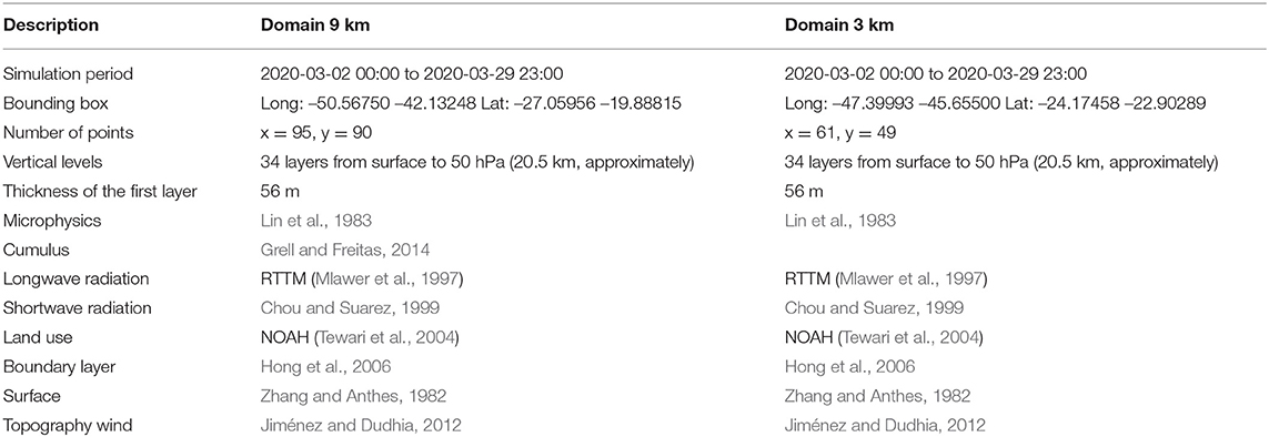
Table 1. Model configuration for WRF-Chem.
Periods of Study
The lockdown restrictions started on March 23 according to the official municipal decree (Estado de São Paulo, 2020). In order to study the effect of lockdown, we estimated the hourly emissions for all hours of March 2020 at each street of the São Paulo metropolitan region. Then, we considered the following periods of days:
• Spin-up: March 02 to March 08.
• Pre-Lockdown: March 09 to March 15.
• Transition: March 16 to 22.
• Lockdown: March 23 to 29.
The spin-up period represents the period of time where the model requires to stabilize. In this way, we are able to compare full weeks, from Monday to Sunday. Finally, we calculated diurnal cycles to each period to understand the volume, emissions, and concentrations.
Results
Traffic Volume
Temporal factors used to interpolate transportation flow for March 2020 are shown in Figure 1 for passenger cars (PC), light commercial vehicles (LCV), light trucks (LT or trucks with 2 axles), medium trucks (MT or trucks with 3 axles), heavy trucks (HT or trucks with more than 4 axles), buses (BUS), and motorcycles (MC). The spatial representation of volumes is shown by Ibarra-Espinosa et al. (2020). We added smooth lines as LOESS regression made with ggplot2 and R (Wickham, 2016; R Core Team, 2021). The trend lines show that the biggest drop is for urban transportation, during Pre-Lockdown, values were about one but during Lockdown 0.5. This is important because buses in Brazil mostly consume diesel, then a decrease in these vehicles could imply less NOX and more favorable conditions to increase ozone. On the contrary, we see those heavy trucks and medium trucks increased circulation during Transition, while medium trucks dropped again, heavy ones remained almost constant. This means that previous to Lockdown, there was an increase in demand for goods and their transportation. There was a decrease in all the other types of vehicles. When we consider the average values during Pre-Lockdown and Lockdown, we see that the drop for PC, MC, and BUS were about 50%, while for LCV 33%, LT 23%, MT 18%, and HT only 1%.

Figure 1. Temporal factors for transportation volume in São Paulo in March 2020 including Passenger Cars (PC), Light Commercial Vehicles (LCV), Light Trucks (LT), Medium Trucks (MT), Heavy Trucks (HT), Buses (BUS), and Motorcycles (MC). Temporal factors are used to extrapolate the morning rush hour volume of transportation.
Air Pollutant Concentrations
In order to obtain an overview of the air pollutant concentrations, we used data from air pollutant observatory stations from CETESB and averaged monthly values for the periods 2019, 2020, and 1998–2018. These averages covered all the stations CERQUEIRA CESAR, CONGONHAS, PARQUE PEDRO II, and IBIRAPUERA, locations shown in Figure 2. The average monthly concentrations, in general, are lower during the years 2019 and 2020 than the historic average for CO, NO2, and NO. In the case of PM10, the values are closer and for PM2.5, the values for 2019 are very similar to the historic, but the 2020 values are still lower, reflecting the impact of COVID-19 on human activity. Finally, the O3 has incremented the concentrations with even higher values during 2020, especially in October. Then, the annual percentage change between 2020 and 2019 for the pollutants CO, NO, NO2, O3, PM10, and PM2.5 was –12.55, –39.06, –19.98, 4.37, 2.39, and –5.5%, respectively. These changes are directly related to the lockdown. However, when comparing 2019 with the average between 1998 and 2018, we see that there is a trend of lower concentrations with the exception of O3. The reasons for the historic changes in air pollutants have been associated with the environmental management in relation to the implementation of clean technologies required by newer emission standards (Carvalho et al., 2015; Fatima Andrade et al., 2017). Furthermore, it has been shown that since 2006 approximately, the O3 had a positive trend for many stations in MASP (Schuch et al., 2019). However, the O3 during 2020 presented a different behavior from the other years. We can see how during March there was a pronounced peak, which seems related to the change in emissions.
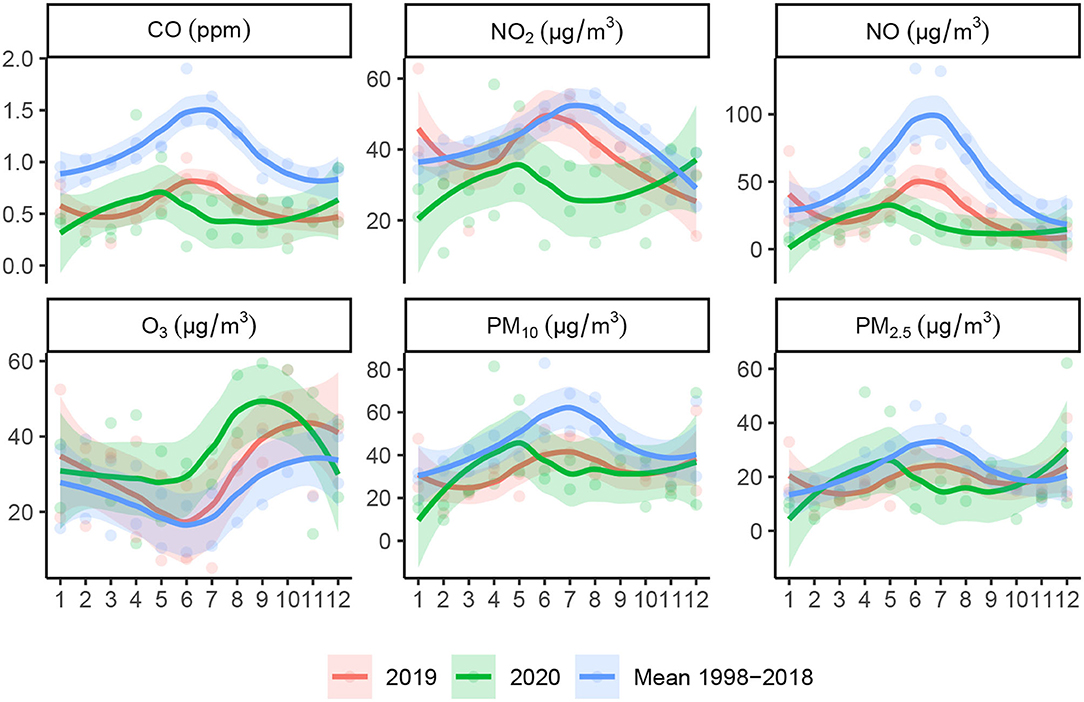
Figure 2. Monthly average air pollutant concentrations in São Paulo for the periods 2020, 2019, and mean 1998–2018. The smooth line represents a LOESS regression (refer to Methods).
Emissions
The emissions inventory adjusted by fuel consumption for March 2020 is shown in Table 2, as the average hourly emissions by period and the percentage difference. Table 2 is also ordered from the highest difference, which occurs for the ethanol (ETOH), followed by ammonia (NH3), carbon monoxide, and non-methanic hydrocarbons, between –52 and –42%. On the other hand, a lower decrease occurred for the nitrogen monoxide, nitrogen dioxide, sulfur dioxide (SO2), and particulate matter (PM10 and PM2.5) with aerodynamic diameters lower than 2.5 μm (PM2.5) with –17, –19, –20, and –24%. Note that the emissions from particulate matter include exhaust and paved roads, NMHC exhaust and evaporative and CO2 is entirely without discount apart from biodiesel (7% on diesel), ethanol, and 27% of ethanol in gasoline.
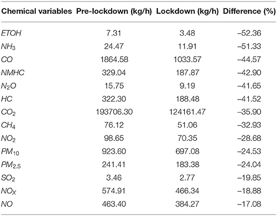
Table 2. Average hourly emissions (kg/h) by the period in MASP.
Despite analyzing the hourly emissions providing good insight, here, we are more interested in the spatio-temporal variations of the emissions. As mentioned before, the decrease in buses might lead to a different spatial pattern after COVID-19. One of the focuses here is to study air pollution and the ratio is of special interest because an increase can favor the production of tropospheric ozone (Alvim et al., 2018). Then, we spatially calculated this ratio with a 3 km grid used by the model WRF-Chem, as shown in Figure 3. The process to allocate emissions with mass conservation is made in the VEIN model3. Figure 3 shows in general a lower ratio and the average value for the whole domain is –19.04%. However, there are some positive areas showing an increment in the ratio, with peaks of 2.7% toward the center of the city. This means that there are areas in the domain that may experience an increase in ozone for the emissions change. For reference, the spatial average change for NMHC was –40.1%, while the change for NOX was –25.8%, meaning that the main reduction was because of the gasoline vehicles.
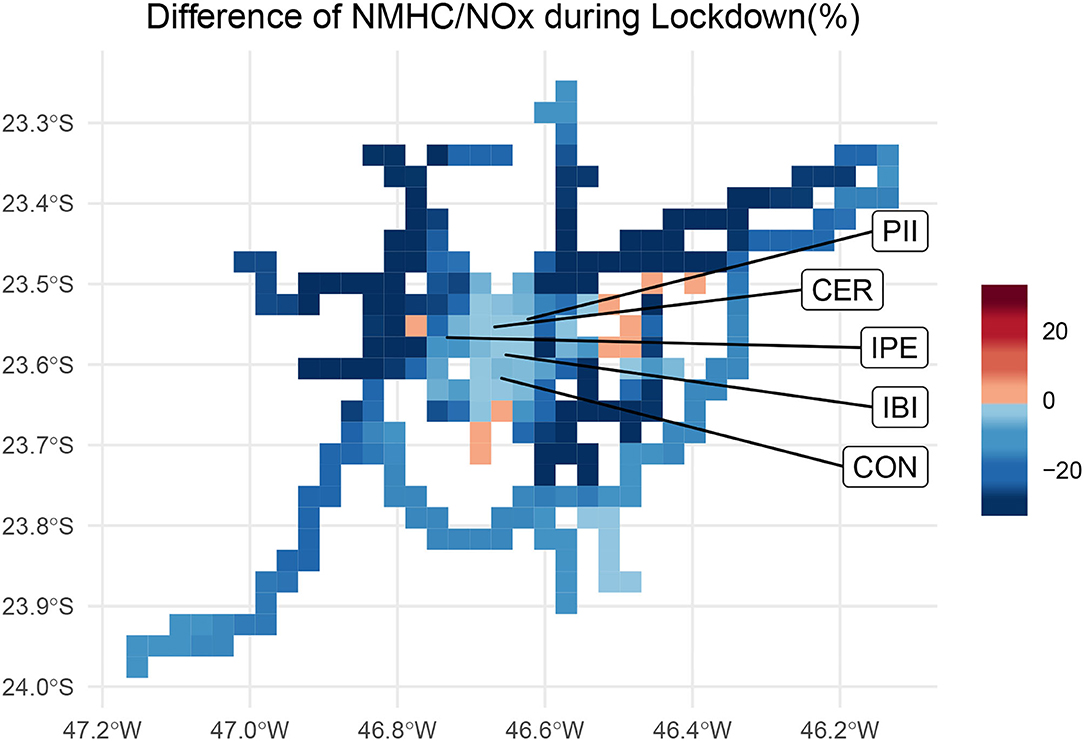
Figure 3. Spatial percentage change of NMHC/NO2 between Pre-Lockdown and Lockdown in São Paulo. The location of the stations PARQUE D.PEDRO II (PII), CERQUEIRA CESAR (CER), IBIRAPUERA (IBI), and CONGONHAS (CON) is also included.
Air Pollution Modeling
The numerical representation of air pollution during the lockdown in São Paulo was challenging because, despite the fact that our estimation covers road transportation, which is the most important source of pollution in this megacity, there is consistently a negative bias. This means that one of the top priorities for the atmospheric and chemistry community in Brazil is to develop inventories of unaccounted sources. Although there are global inventories to fill missing sources, these are known to have inconsistencies for Latin America, with lower emissions than local inventories (Madrazo et al., 2018). Figure 4 shows the diurnal cycle comparison between observation as CETESB and the simulations for the whole period, without spin up for CO (ppm), NO (μgm−3), and O3 (μgm−3) by a chemical mechanism. We can see how the CO is the pollutant with the largest under prediction and how there is no difference among chemical mechanisms, but the better agreement occurs in the urban station of PARQUE D.PEDRO II. In the case of NO, there is an agreement between stations IBIRAPUERA, which is located inside an urban park, and the urban station PARQUE D.PEDRO II. However, the NO morning peak is still underestimated, probably related to the planetary boundary layer and winds, although this type of analysis is out of the scope of this study. Again, there is quite agreement between different chemical mechanisms for NO. Finally, the O3 is underestimated, which might be related to the overprediction of wind speed (Ibarra-Espinosa et al., 2022b), the underestimation of urban non-methanic hydrocarbons, and the underestimation of urban NMHC. Actually, McDonald et al. (2018) show that the volatile chemical products, which are precursors of ozone, are largely underestimated. However, the diurnal cycle is well represented in the stations with the best agreement in station Parque D.PEDRO II and IBIRAPUERA. Regarding the chemical mechanisms, we do see differences with better results for RADM2 followed by CBMZ. Please, note that the station CONGONHAS is located near the CONGONHAS airport (http://www.aeroportocongonhas.net/) and includes many stationary and aircraft emission sources which are not considered in this study.
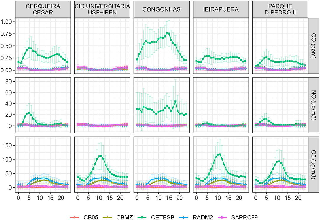
Figure 4. Dournal cycles during March 2020 for CO, NO, and ozone, São Paulo. The points represent the averages and the vertical lines, the standard deviation.
After taking a look at the general performance of the air pollution modeling, now it is time to see if the models are able to represent the air pollutant concentrations at different Lockdown periods. Figure 5 shows the diurnal cycle for the period, chemical mechanism, and pollutant in March 2020 for the urban station PARQUE D.PEDRO II. The observations are shown in the facet CETESB, where we can see that the CO was different for the periods, with similar values during Pre-Lockdown and Transition and 50% fewer concentrations during Lockdown. The different mechanisms also presented lower concentrations during Lockdown, but in this case, very similar values with Transition. Then, the chemical mechanism which presented the closest decrease with CO was SAPRC99, with 33%. The observed NO had similar values in this station for all the periods, with higher concentrations during the Transition phase. The mechanisms RADM2 had a sharp peak with similar values for all phases, SAPRC99 and CB05 were able to modestly improve the representation of the smooth peak. Furthermore, except for RADM2, all mechanisms overestimated concentrations at night time. The observed change during Lockdown was –20% and the closest change was obtained with CB05, which was –19.5%. The observed O3 has a marked diurnal profile with higher concentrations during Pre-Lockdown, followed by Transition and Lockdown. The observed change was decreased by –33% and the closest mechanism was RADM2 with –46%. Regarding the shape, CBMZ performed better followed by RADM2, while SAPRC99 was the only one with Transition and Pre-Lockdown values similar. It was not possible to generate ozone with CB05 and currently, we are studying the causes.
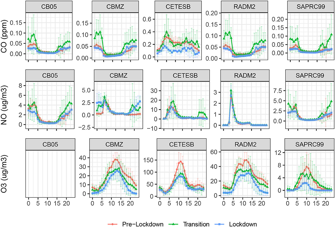
Figure 5. Simulated diurnal cycle during Lockdown periods in March 2020 São Paulo for the chemical mechanisms CB05, CBMZ, RADM2, SAPRC99, and observations from CETESB. The points represent the averages and the vertical lines, the standard deviation.
Discussion and Conclusion
In this study, we have presented a bottom-up vehicular emissions inventory for the megacity of São Paulo, characterizing the street emissions during all hours of March 2020. This was possible because we obtained hourly traffic counts for the whole hours of March 2020, plus volumes at each street. We also obtained vehicular fuel consumption for the area of study to calibrate the activity data. There are still challenges to improving the emissions estimation, among them counting temporal factors for each street. Despite the limitations, it was possible to develop and perform a detailed spatial and temporal characterization of vehicular emissionsat street level. Furthermore, the map allowed us to identify that there are areas near downtown where the lockdown increased this ratio, favoring the conditions for ozone production.
The reductions found in the vehicular emissions due to lockdown align with other published studies. For instance, Guevara et al. (2021) found that NO2, which is very characteristic of vehicular emissions, was reduced by –33% while we found by –29%. An evaluation of vehicular emissions in Bogota, Colombia, showed that during the lockdown, the emissions of CO, PM10, NO2, SO2, and PM2.5 were reduced by 29%, 21%, 18%, 16%, and 11%, respectively} (Pardo-Amaya and Stephen, 2022), while our reductions for the same pollutants were –44, –25, –29, –20, and –24%. Therefore, oyr dynamic inventory was able to represent the complex emissions changes during the lockdown.
In our study, the pollutants with the highest reductions were, ETOH, NH3, and CO. According to the CETESB emission factors, these pollutants are emitted mainly by light vehicles. Then, as the light fleet, which are the PC, MC, and LCV, experimented with the strongest reduction in circulation, with –50, –50, and –33%, this explains why these pollutants suffer more reductions. In contrast, the main emitters of NOX and PM2.5 are the trucks, which experimented with a reduction between –20 and –1%, hence, presenting a smaller impact of these pollutants. The Supplementary Material shows the emission factors (g/km) by age of use used in this study.
Vehicular emissions estimation can also be improved by incorporating emission factors that depend on the kinematics of traffic volumes such as speed, traffic situation, or vehicular specific power (VSP) (Franco et al., 2013). The speed approach consists of the emission factors as speed functions. The traffic situation approach identifies emission factors by a combination of the type of vehicle, level of congestion, speed limit, category, and type of street and more characteristics. Then, this approach allows more flexibility than speed functions. The VSP approach combines power and many characteristics of a vehicle to represent vehicular emissions on a second-by-second basis. However, we consider that the most critical aspect to improve the emissions is to incorporate all the missing sources, other than vehicles. As explained by McDonald et al. (2018), the trend in vehicular emissions is to decrease because of the surge of new technologies, which led to the rise of emergent new sources such as the volatile chemical products. There are some efforts in Brazil to add different sources, such as the System for Estimating Greenhouse Gas Emissions (SEEG) (De Azevedo et al., 2018), which provides a simple yet powerful way to report emissions from different sources in Brazil with a top-down approach. Using an explicit and spatial approach, Kawashima et al. (2020) presented an industry inventory for Brazil. There are some efforts to characterize the emissions from pizza restaurants in Brazil, which are an important source of particulate matter since they are numerous (Lima et al., 2020). However, there are still many sources to be included in a unique system, such as Convention on Long-Range Transboundary Air Pollution, in which the parties are required to report their emissions annually (Rosencranz, 1981).
The observations of air pollutants show during the year 2020, lower concentrations were found in comparison with 2019. The annual percentage change between 2020 and 2019 for the pollutants CO, NO, NO2, O3, PM10, and PM2.5 was –12.55, –39.06, –19.98, 4.37, 2.39, and –5.5%, respectively. It has been documented that the increment of O3 is related to the reduction in NOX (Wang et al., 2021). The air quality simulations, in general, were lower than observations with few exceptions as in the station PARQUE D.PEDRO II. Nevertheless, in general, the simulations represented the diurnal cycle. Best agreement was found for NO and the stations IBIRAPUERA and PARQUE D.PEDRO II. The chemical mechanisms that simulated better the O3 were CBMZ and RADM2. Indeed, RADM2 reaches higher concentrations than CBMZ, however, CBMZ simulates the diurnal cycle more than RADM2. The concentrations simulated by SAPRC99 were lower and with a more different diurnal cycle. The chemical mechanism with the best performance was CBMZ. Other studies that compare mechanisms may have different results because of the air pollution model and the quality of the input data. For instance, Chen et al. (2021) used the Community Multiscale Air Quality Modeling System (CMAQ) model (Appel et al., 2017) to compare RADM2 and RACM mechanisms with and without updated photolysis rate, finding that RACM achieved better results to predict ozone. Also, Luecken et al. (2008) found that SAPRC99 and CB05 performed better than CB4 mechanisms over the US to predict air pollutants. PM2.5 is a pollutant with a deleterious effect on human health (Dominici et al., 2006). Furthermore, PM2.5 can have different origins and be generated in the atmosphere as a secondary pollutant Hyde et al. (2018); Hyde and Mahalov (2020). Then, future studies must consider this pollutant accounting for the complex environmental interactions. The Metropolitan Area of São Paulo consists of a tropical megacity strongly influenced by south American monoson and mesoscale circulations (Freitas et al., 2007). Then, despite that our results align with published literature, more research is needed to confirm if these results are representative of other cities with similar conditions, especially in the context of COVID-19.
Simulating health policy decisions such as Lockdown on air quality has been a challenge because we depend on the quality of input data, models representative, and good observation data. All model experiments identify the different phases being Pre-Lockdown, Transition, and Lockdown, as observed. All the observations and simulations presented lower concentrations during Lockdown. The only case was NO simulations were higher than the other phases, at night time for CBMZ. The CO observations show higher concentrations during Pre-Lockdown and Transition, and lower during Lockdown, while during simulations only Transition reached the highest values. The NO concentrations obtained with RADM2 were too similar and it is not possible to differentiate phases. In the case of O3, despite those simulations being lower than observations, RADM2 actually was closer followed by CBMZ. The result of this study suggests that, in order to reduce air pollutant concentrations, different strategies must be adapted according to each pollutant.
Data Availability Statement
The raw data supporting the conclusions of this article will be made available by the authors, without undue reservation.
Author Contributions
SI-E, AR, and ED: conceptualization and software. SI-E, AR, ED, EL, LM, and MA: methodology. SI-E, AR, ED, MA, EL, and LM: validation. SI-E, AR, ED, MA, and EL: formal analysis, investigation, data curation, and visualization. SI-E, ED, MA, and EL: resources, writing—original draft preparation, supervision, project administration, funding acquisition, and writing—review and editing. All authors have read and agreed to the published version of the manuscript.
Funding
ED efforts were supported by the São Paulo Research Foundation (FAPESP) (Grants Nos. 2015/03804-9 and 2016/18438-0) and CNPq (Grant No. 309514/2019-3), AR efforts were also supported by FAPESP (Grant Nos. 2016/10557-0 and 2021/07992-5), and SI-E efforts were also supported by FAPESP (Grant No. 2021/07136-1).
Conflict of Interest
The authors declare that the research was conducted in the absence of any commercial or financial relationships that could be construed as a potential conflict of interest.
Publisher's Note
All claims expressed in this article are solely those of the authors and do not necessarily represent those of their affiliated organizations, or those of the publisher, the editors and the reviewers. Any product that may be evaluated in this article, or claim that may be made by its manufacturer, is not guaranteed or endorsed by the publisher.
Supplementary Material
The Supplementary Material for this article can be found online at: https://www.frontiersin.org/articles/10.3389/frsc.2022.883112/full#supplementary-material
Footnotes
1. ^https://atmoschem.github.io/vein/reference/speciate.html
2. ^https://atmoschem.github.io/vein/reference/emis/_chem2.html
3. ^https://atmoschem.github.io/vein/reference/emis_grid.html
References
Alfano, V., and Ercolano, S. (2020). The efficacy of lockdown against COVID-19: a cross-country panel analysis. Appl. Health Econ. Health Policy 18, 509–517. doi: 10.1007/s40258-020-00596-3
Alvim, D. S., Gatti, L. V., Corrêa, S. M., Chiquetto, J. B., Santos, G. M., Souza Rossatti, C., et al. (2018). Determining VOCs reactivity for ozone forming potential in the megacity of são paulo. Aerosol Air Qual. Res. 18, 2460–2474. doi: 10.4209/aaqr.2017.10.0361
Andrade, M., de, F., Ynoue, R. Y., Freitas, E. D., Todesco, E., Vara Vela, A., et al. (2015). Air quality forecasting system for Southeastern Brazil. Front. Environ. Sci. 3, 9. doi: 10.3389/fenvs.2015.00009
Appel, K. W., Napelenok, S. L., Foley, K. M., Pye, H. O., Hogrefe, C., Luecken, D. J., et al. (2017). Description and evaluation of the community multiscale air quality (CMAQ) modeling system version 5.1. Geoscientific Model Dev. 10, 1703–1732. doi: 10.5194/gmd-10-1703-2017
Apple. (2022). Community Mobility Reports. Available online at: https://COVID19.apple.com/mobility (accessed January 28, 2022).
Bao, R., and Zhang, A. (2020). Does lockdown reduce air pollution? Evidence from 44 cities in northern china. Sci. Total Environ. 731, 139052. doi: 10.1016/j.scitotenv.2020.139052
Barua, S., and Nath, S. D. (2021). The impact of COVID-19 on air pollution: evidence from global data. J. Clean Prod. 298, 126755. doi: 10.1016/j.jclepro.2021.126755
Biroli, P., Bosworth, S., Della Giusta, M., Di Girolamo, A., Jaworska, S., and Vollen, J. (2021). Family life in lockdown. Front. Psychol. 12, 687570. doi: 10.3389/fpsyg.2021.687570
Carter, W. P.. (2000). Implementation of the SAPRC-99 chemical mechanism into the models-3 framework. Report to the United States Environmental Protection Agency, January 29.
Carter, W. P.. (2015). Development of a database for chemical mechanism assignments for volatile organic emissions. J. Air Waste Manag. Assoc.65, 1171–1184. doi: 10.1080/10962247.2015.1013646
Carvalho, V. S. B., Freitas, E. D., Martins, L. D., Martins, J. A., Mazzoli, C. R., and Fátima Andrade, M. d. (2015). Air quality status and trends over the metropolitan area of São Paulo, Brazil as a result of emission control policies. Environ. Sci. Policy 47, 68–79. doi: 10.1016/j.envsci.2014.11.001
CETESB (2020). Emissões Veiculares no Estado de São Paulo 2020. Available online at: https://cetesb.sp.gov.br/veicular/relatorios-e-publicacoes/
Chan, J. F.-W., Yuan, S., Kok, K.-H., To, K. K.-W., Chu, H., Yang, J., et al. (2020). A familial cluster of pneumonia associated with the 2019 novel coronavirus indicating person-to-person transmission: a study of a family cluster. Lancet 395, 514–523. doi: 10.1016/S0140-6736(20)30154-9
Chen, C.-H., Chen, T.-F., Huang, S.-P., and Chang, K.-H. (2021). Comparison of the RADM2 and RACM chemical mechanisms in O3 simulations: effect of the photolysis rate constant. Scientific Rep. 11, 1–15. doi: 10.1038/s41598-021-84629-4
Chou, M. -D., and Suarez, M. J. (1999). A Solar Radiation Parameterization for Atmospheric Studies. No. NASA/TM-1999-104606/VOL15. Available online at: https://ntrs.nasa.gov/citations/19990060930
Crippa, M., Solazzo, E., Huang, G., Guizzardi, D., Koffi, E., Muntean, M., et al. (2020). High resolution temporal profiles in the emissions database for global atmospheric research. Scientific Data 7, 1–17. doi: 10.1038/s41597-020-0462-2
Danabasoglu, G., Lamarque, J.-F., Bacmeister, J., Bailey, D., DuVivier, A., Edwards, J., et al. (2020). The community earth system model version 2 (CESM2). J. Adv. Model. Earth Syst. 12, e2019MS001916. doi: 10.1029/2019MS001916
De Azevedo, T. R., Costa Junior, C., Brandão Junior, A., Cremer, M., dos, S., Piatto, M., et al. (2018). SEEG initiative estimates of Brazilian greenhouse gas emissions from 1970 to 2015. Scientific Data 5, 1–43. doi: 10.1038/sdata.2018.45
Dominici, F., Peng, R. D., Bell, M. L., Pham, L., McDermott, A., Zeger, S. L., et al. (2006). Fine particulate air pollution and hospital admission for cardiovascular and respiratory diseases. JAMA 295, 1127–1134. doi: 10.1001/jama.295.10.1127
Dong, E., Du, H., and Gardner, L. (2020). An interactive web-based dashboard to track COVID-19 in real time. Lancet Infect. Dis. 20, 533–534. doi: 10.1016/S1473-3099(20)30120-1
Estado de São Paulo, G. d.. (2020). Decreta quarentena no estado de são paulo, no contexto da pandemia do COVID-19. Available online at: https://www.saopaulo.sp.gov.br/coronavirus/ (accessed February 15, 2022).
Fatima Andrade, M., de Kumar, P., Freitas, E. D., de Ynoue, R. Y., Martins, J., Martins, L. D., et al. (2017). Air quality in the megacity of são paulo: evolution over the last 30 years and future perspectives. Atmosphere. Environ. 159, 66–82. doi: 10.1016/j.atmosenv.2017.03.051
Forster, P. M., Forster, H. I., Evans, M. J., Gidden, M. J., Jones, C. D., Keller, C. A., et al. (2020). Current and future global climate impacts resulting from COVID-19. Nat. Climate Change 10, 913–919. doi: 10.1038/s41558-020-0883-0
Franco, V., Kousoulidou, M., Muntean, M., Ntziachristos, L., Hausberger, S., and Dilara, P. (2013). Road vehicle emission factors development: a review. Atmosphere. Environ. 70, 84–97. doi: 10.1016/j.atmosenv.2013.01.006
Freitas, E. D., Rozoff, C. M., Cotton, W. R., and Dias, P. L. S. (2007). Interactions of an urban heat island and sea-breeze circulations during winter over the metropolitan area of São Paulo, Brazil. Boundarylayer Meteorol. 122, 43–65. doi: 10.1007/s10546-006-9091-3
Gettelman, A., Lamboll, R., Bardeen, C., Forster, P., and Watson-Parris, D. (2021). Climate impacts of COVID-19 induced emission changes. Geophys. Res. Lett. 48, e2020GL091805. doi: 10.1029/2020GL091805
Google (2022). Community Mobility Reports. Available online at: https://www.google.com/COVID19/mobility/ (accessed January 28, 2022).
Grange, S. K., Lee, J. D., Drysdale, W. S., Lewis, A. C., Hueglin, C., Emmenegger, L., et al. (2021). COVID-19 lockdowns highlight a risk of increasing ozone pollution in european urban areas. Atmosphere. Chem. Phys. 21, 4169–4185. doi: 10.5194/acp-21-4169-2021
Grell, G. A., and Freitas, S. R. (2014). A scale and aerosol aware stochastic convective parameterization for weather and air quality modeling. Atmosphere. Chem. Phys. 14, 5233–5250. doi: 10.5194/acp-14-5233-2014
Grell, G. A., Peckham, S. E., Schmitz, R., McKeen, S. A., Frost, G., Skamarock, W. C., et al. (2005). Fully coupled “online” chemistry within the WRF model. Atmosphere. Environ. 39, 6957–6975. doi: 10.1016/j.atmosenv.2005.04.027
Guevara, M., Jorba, O., Soret, A., Petetin, H., Bowdalo, D., Serradell, K., et al. (2021). Time-resolved emission reductions for atmospheric chemistry modelling in europe during the COVID-19 lockdowns. Atmosphere. Chem. Phys. 21, 773–797. doi: 10.5194/acp-21-773-2021
Hernandez-Paniagua, I. Y., Valdez, S. I., Almanza, V., Rivera-Cardenas, C., Grutter, M., Stremme, W., et al. (2021). Impact of the COVID-19 lockdown on air quality and resulting public health benefits in the mexico city metropolitan area. Front. Public Health 9, 242. doi: 10.3389/fpubh.2021.642630
Hong, S.-Y., Noh, Y., and Dudhia, J. (2006). A new vertical diffusion package with an explicit treatment of entrainment processes. Month. Weather Rev. 134, 2318–2341. doi: 10.1175/MWR3199.1
Hyde, P., and Mahalov, A. (2020). Contribution of bioaerosols to airborne particulate matter. J. Air Waste Manag. Assoc. 70, 71–77. doi: 10.1080/10962247.2019.1629360
Hyde, P., Mahalov, A., and Li, J. (2018). Simulating the meteorology and PM10 concentrations in arizona dust storms using the weather research and forecasting model with chemistry (wrf-chem). J. Air Waste Manag. Assoc. 68, 177–195. doi: 10.1080/10962247.2017.1357662
Ibarra-Espinosa, S., Freitas, E. D., de Ropkins, K., Dominici, F., and Rehbein, A. (2022a). Negative-binomial and quasi-poisson regressions between COVID-19, mobility and environment in São Paulo, Brazil. Environ. Res. 204, 112369. doi: 10.1016/j.envres.2021.112369
Ibarra-Espinosa, S., Mendes da Silva, G. A., Rehbein, A., Vara-Vela, A., and Dias de Freitas, E. (2022b). Atmospheric effects of air pollution during dry and wet periods in são paulo. Environ. Sci. Atmospheres 2, 215–229. doi: 10.1039/D1EA00080B
Ibarra-Espinosa, S., and Ropkins, K. (2021). Respeciate: Speciation Profiles for Gases and Aerosols. Available online at: https://github.com/atmoschem/respeciate
Ibarra-Espinosa, S., Ynoue, R., OSullivan, S., Pebesma, E., Andrade, M., de, F., et al. (2018). VEIN v0. 2.2: an r package for bottom–up vehicular emissions inventories. Geoscientific Model Dev. 11, 2209–2229. doi: 10.5194/gmd-11-2209-2018
Ibarra-Espinosa, S., Ynoue, R. Y., Ropkins, K., Zhang, X., and Freitas, E. D. de (2020). High spatial and temporal resolution vehicular emissions in South-East Brazil with traffic data from real-time GPS and travel demand models. Atmos Environ. 222, 117136. doi: 10.1016/j.atmosenv.2019.117136
IEA (2022). Global Energy Review 2020. Available online at: https://www.iea.org/reports/global-energy-review-2020
Infectious Diseases, I. S.. (2019). Undiagnosed Pneumonia–China (Hubei): Request for Information. Available online at: https://promedmail.org/promed-post/?id=6864153
Jiménez, P. A., and Dudhia, J. (2012). Improving the representation of resolved and unresolved topographic effects on surface wind in the WRF model. J. Appl. Meteorol. Climatol. 51, 300–316. doi: 10.1175/JAMC-D-11-084.1
Kawashima, A. B., Martins, L. D., Rafee, S. A. A., Rudke, A. P., Morais, M. d. V., and Martins, J. A. (2020). Development of a spatialized atmospheric emission inventory for the main industrial sources in Brazil. Environ. Sci. Pollut. Res. 27, 35941–35951. doi: 10.1007/s11356-020-08281-7
Li, J., Georgescu, M., Hyde, P., Mahalov, A., and Moustaoui, M. (2015). Regional-scale transport of air pollutants: IM|pacts of southern california emissions on phoenix ground-level ozone concentrations. Atmosphere. Chem. Phys. 15, 9345–9360. doi: 10.5194/acp-15-9345-2015
Lima, F. D. M., Perez-Martinez, P. J., Fatima Andrade, M., de Kumar, P., and Miranda, R. d. M. (2020). Characterization of particles emitted by pizzerias burning wood and briquettes: a case study at São Paulo, Brazil. Environ. Sci. Pollut. Res. 27, 35875–35888. doi: 10.1007/s11356-019-07508-6
Lin, Y.-L., Farley, R. D., and Orville, H. D. (1983). Bulk parameterization of the snow field in a cloud model. J. Appl. Meteorol. Climatol. 22, 1065–1092. doi: 10.1175/1520-0450(1983)022andlt;1065:BPOTSFandgt;2.0.CO;2
Luecken, D. J., Phillips, S., Sarwar, G., and Jang, C. (2008). Effects of using the CB05 vs. SAPRC99 vs. CB4 chemical mechanism on model predictions: ozone and gas-phase photochemical precursor concentrations. Atmosphere. Environ. 42, 5805–5820. doi: 10.1016/j.atmosenv.2007.08.056
Madrazo, J., Clappier, A., Belalcazar, L. C., Cuesta, O., Contreras, H., and Golay, F. (2018). Screening differences between a local inventory and the emissions database for global atmospheric research (EDGAR). Sci. Total Environm. 631, 934–941. doi: 10.1016/j.scitotenv.2018.03.094
Martins, L. D., Andrade, M. F., Freitas, E. D., Pretto, A., Gatti, L. V., Albuquerque, É. L., et al. (2006). Emission factors for gas-powered vehicles traveling through road tunnels in São Paulo, Brazil. Environ. Sci. Technol. 40, 6722–6729. doi: 10.1021/es052441u
Martins, L. D., and Fátima Andrade, M. de (2008). Ozone formation potentials of volatile organic compounds and ozone sensitivity to their emission in the megacity of São Paulo, Brazil. Water Air Soil Pollut. 195, 201–213. doi: 10.1007/s11270-008-9740-x
McDonald, B. C., De Gouw, J. A., Gilman, J. B., Jathar, S. H., Akherati, A., Cappa, C. D., et al. (2018). Volatile chemical products emerging as largest petrochemical source of urban organic emissions. Science 359, 760–764. doi: 10.1126/science.aaq0524
Mlawer, E. J., Taubman, S. J., Brown, P. D., Iacono, M. J., and Clough, S. A. (1997). Radiative transfer for inhomogeneous atmospheres: RRTM, a validated correlated-k model for the longwave. J. Geophys. Res. 102, 16663–16682. doi: 10.1029/97JD00237
National Centers for Environmental Prediction National Weather Service NOAA, U.S. Department of Commerce. (2000). NCEP FNL Operational Model Global Tropospheric Analyses, Continuing From July 1999. Available online at: https://doi.org/10.5065/D6M043C6
National Centers for Environmental Prediction National Weather Service, NOAA, U.S. Department of Commerce. (2015). NCEP GDAS/FNL 0.25 Degree Global Tropospheric Analyses and Forecast Grids.
Nogueira, T., de Souza, K. F., Fornaro, A., de Fatima Andrade, M., and de Carvalho, L. R. F. (2015). On-road emissions of carbonyls from vehicles powered by biofuel blends in traffic tunnels in the metropolitan area of São Paulo, Brazil. Atmosphere. Environ. 108, 88–97. doi: 10.1016/j.atmosenv.2015.02.064
Pardo-Amaya, D., and Stephen, S. (2022). Assessment of the impact of vehicle emissions on air quality changes during COVID-19 lockdown in Bogota, Colombia. WCX SAE World Congress Experience. Oxford Brookes University. Available online at: https://www.sae.org/publications/technical-papers/content/2022-01-0583/
R Core Team (2021). R: A Language and Environment for Statistical Computing. Vienna: R Foundation for Statistical Computing. Available online at: https://www.R-project.org/
Rosencranz, A.. (1981). The ECE convention of 1979 on long-range transboundary air pollution. Am. J. Int. Law 75, 975–982. doi: 10.2307/2201373
Schuch, D., de Freitas, E. D., Ibarra-Espinosa, S., Martins, L. D., Carvalho, V. S. B., Ramin, B. F., et al. (2019). A two decades study on ozone variability and trend over the main urban areas of the São Paulo state, Brazil. Environ. Sci. Pollut. Res. 26, 31699–31716. doi: 10.1007/s11356-019-06200-z
Simon, H., Beck, L., Bhave, P. V., Divita, F., Hsu, Y., Luecken, D., et al. (2010). The development and uses of EPA's SPECIATE database. Atmosphere. Pollut. Res. 1, 196–206. doi: 10.5094/APR.2010.026
Skamarock, W. C., Klemp, J. B., Dudhia, J., Gill, D. O., Barker, D. M., Wang, W., et al. (2005). A description of the advanced research WRF version 2. Boulder, CO: NCAR Mesoscale and Microscale Meteorology Div. Available online at: https://apps.dtic.mil/sti/pdfs/ADA487419.pdf
Sokhi, R. S., Singh, V., Querol, X., Finardi, S., Targino, A. C., Fatima Andrade, M., et al. (2021). A global observational analysis to understand changes in air quality during exceptionally low anthropogenic emission conditions. Environ. Int. 157, 106818. doi: 10.1016/j.envint.2021.106818
Stockwell, W. R., Middleton, P., Chang, J. S., and Tang, X. (1990). The second generation regional acid deposition model chemical mechanism for regional air quality modeling. J. Geophys. Res. 95, 16343–16367. doi: 10.1029/JD095iD10p16343
Tewari, M., Chen, F., Wang, W., Dudhia, J., Lemone, M. A., et al. (2004). “Implementation and verification of the unified NOAH land surface model in the WRF model (Formerly Paper Number 17.5),” in Proceedings of the 20th Conference on Weather Analysis and Forecasting/16th Conference on Numerical Weather Prediction (Seattle, WA). Available online at: https://ams.confex.com/ams/84Annual/techprogram/program_185.htm
Thunis, P., Clappier, A., Meij, A., de Pisoni, E., Bessagnet, B., and Tarrason, L. (2021). Why is the city's responsibility for its air pollution often underestimated? A focus on PM2.5. Atmosphere. Chem. Phys. 21, 18195–18212. doi: 10.5194/acp-21-18195-2021
USA-EPA. (2016). AP42 compilation of emission factors; Miscellaneous Sources. 13.2.1 Paved Roads. Environment Protection Agency. Available online at: https://www.epa.gov/sites/default/files/2020-10/documents/13.2.1_paved_roads.pdf
Venter, Z. S., Aunan, K., Chowdhury, S., and Lelieveld, J. (2020). COVID-19 lockdowns cause global air pollution declines. Proc. Natl. Acad. Sci. U.S.A. 117, 18984–18990. doi: 10.1073/pnas.2006853117
Wang, C., Horby, P. W., Hayden, F. G., and Gao, G. F. (2020). A novel coronavirus outbreak of global health concern. Lancet 395, 470–473. doi: 10.1016/S0140-6736(20)30185-9
Wang, N., Xu, J., Pei, C., Tang, R., Zhou, D., Chen, Y., et al. (2021). Air quality during COVID-19 lockdown in the yangtze river delta and the pearl river delta: Two different responsive mechanisms to emission reductions in China. Environ. Sci. Technol. 55, 5721–5730. doi: 10.1021/acs.est.0c08383
Wickham, H.. (2016). ggplot2: Elegant Graphics for Data Analysis. New York, NY: Springer-Verlag. Available online at: https://ggplot2.tidyverse.org
Yarwood, G., Rao, S., Yocke, M., and Whitten, G. (2005). Updates to the Carbon Bond Chemical Mechanism: CB05. Final report to the US EPA, RT-0400675 8, 13.
Zaveri, R. A., and Peters, L. K. (1999). A new lumped structure photochemical mechanism for large-scale applications. J. Geophys. Res. 104, 30387–30415. doi: 10.1029/1999JD900876
Keywords: air pollution, COVID-19, emissions, lockdown, VEIN, WRF-Chem
Citation: Ibarra-Espinosa S, Rehbein A, Freitas ED, Martins L, Andrade MF and Landulfo E (2022) Changes in a Bottom-Up Vehicular Emissions Inventory and Its Impact on Air Pollution During COVID-19 Lockdown in São Paulo, Brazil. Front. Sustain. Cities 4:883112. doi: 10.3389/frsc.2022.883112
Received: 24 February 2022; Accepted: 20 June 2022;
Published: 18 July 2022.
Edited by:
Prashant Kumar, University of Surrey, United KingdomReviewed by:
Tanbir Singh, Research Institute for Humanity and Nature, JapanAlex Mahalov, Arizona State University, United States
Asish Saha, University of Burdwan, India
Copyright © 2022 Ibarra-Espinosa, Rehbein, Freitas, Martins, Andrade and Landulfo. This is an open-access article distributed under the terms of the Creative Commons Attribution License (CC BY). The use, distribution or reproduction in other forums is permitted, provided the original author(s) and the copyright owner(s) are credited and that the original publication in this journal is cited, in accordance with accepted academic practice. No use, distribution or reproduction is permitted which does not comply with these terms.
*Correspondence: Sergio Ibarra-Espinosa, sergio.ibarra-espinosa@noaa.gov