Article

A Spatial-Temporal Model for the Evolution of the COVID-19 Pandemic in Spain Including Mobility

Departament de Matemàtiques, Universitat de València, Av. Vicent Andrés Estellés, E-46100 Burjassot, Spain
*
Author to whom correspondence should be addressed.
Mathematics 2020, 8(10), 1677; https://doi.org/10.3390/math8101677
Submission received: 20 August 2020 / Revised: 19 September 2020 / Accepted: 23 September 2020 / Published: 1 October 2020
(This article belongs to the Special Issue Modeling and Numerical Analysis of Energy and Environment)

Abstract

:
In this work, a model for the simulation of infectious disease outbreaks including mobility data is presented. The model is based on the SAIR compartmental model and includes mobility data terms that model the flow of people between different regions. The aim of the model is to analyze the influence of mobility on the evolution of a disease after a lockdown period and to study the appearance of small epidemic outbreaks due to the so-called imported cases. We apply the model to the simulation of the COVID-19 in the various areas of Spain, for which the authorities made available mobility data based on the position of cell phones. We also introduce a method for the estimation of incomplete mobility data. Some numerical experiments show the importance of data completion and indicate that the model is able to qualitatively simulate the spread tendencies of small outbreaks. This work was motivated by an open call made to the mathematical community in Spain to help predict the spread of the epidemic.

1. Introduction

1.1. Motivation and Scope

On 31 December 2019, the World Health Organization (WHO) office in the People’s Republic of China got an statement from the Wuhan Municipal Health Commission reporting cases of ‘viral pneumonia’ in Wuhan. Since then, the disease, known today as COVID-19, caused by the SARS-CoV-2 virus, has become a part of everyone’s daily life by now. The COVID-19 was declared pandemic by the WHO on 11 March 2020.
In Spain, the first case of COVID-19 was diagnosed on 31 January 2020. During February, the number of infected people increased quickly, as well as the number of deaths, and on 14 March 2020 the state of alarm was declared and a lockdown was imposed on all the country as a drastic measure to dramatically reduce the spread of the disease. From that day on, people should stay at home and only indispensable trips within their hometowns were allowed. All flights from or to Spain were canceled, except the ones launched by the government bringing people home. However, some essential activities were allowed as, for instance road transportation of goods or harvesting fruits and vegetables to export them.
These strict mobility measures were lessened gradually. A four-phase de-escalation plan was designed by the government and applied from 2 May 2020 to 22 June 2020, when the state of alarm ended, along with the lockdown and mobility restrictions. Each phase consisted on different contention policies. Regarding mobility, the most important changes came with the second phase (Phase 1) that allowed people to travel freely inside their province and with the third phase (Phase 2) that allowed people to travel freely through all the country. It is important to remark that mobility was permitted as long as no symptoms of the infection were shown.
Answering the call from the Comité Español de Matemáticas, (CEMat, Spanish Committee of Mathematics, see http://matematicas.uclm.es/cemat/covid19/en/), it is the purpose of this paper to model the spreading of the COVID-19 virus in Spain, focusing on the impact of the mobility restrictions imposed to the population during the state of alarm. This work is based on previous research on the spread of the 2009 A/H1N1 influenza pandemic in Chile [1].
To estimate the impact of people’s mobility on the evolution and spread of the COVID-19 disease, it is really important to have access to real mobility data, so that models that include mobility data terms with parameters that can be tuned or estimated from said real data can be used. The Spanish National Institute of Statistics (INE) gave access to the research community to some mobility data obtained from the position of cell phones. These data were provided by the three major phone companies in Spain, covering around 80% of the total operating smartphones in the country.
The provided data divide the country in smaller areas, depending on the density of population, and give information about the flux of people moving from their residency area to another one during the state of alarm. These data can be compared with the same fluxes happening on a normal day, before the mobility restrictions, to study how these mobility restrictions imposed really affected the spread of the infection.
In accordance with the mobility data at hand, the model presented in this work divides the spatial domain under consideration into an arbitrary number C N of smaller pieces, called mobility areas, corresponding to the mobility areas defined in the data provided by the INE or to aggregates of them. Moreover, the population will be also divided into groups by means of a compartmental model, that will be defined for each mobility area under consideration.
The mobility model described in this work is strongly influenced by the nature of the mobility data supplied by the authorities. The model can be applied to any other country or region as far as similar mobility fluxes are available or can be reliably estimated.

1.2. Related Work

The most used models for disease transmission are compartmental models. In compartmental models for epidemiology [2,3,4] a population is divided into groups (called compartments) according to the state in which individuals are regarding the disease. The model is defined by the type of compartments considered and by the statement of the ways in which individuals may change from one compartment to another. Both issues are strongly influenced by the particular disease under consideration, but different models, based on different hypotheses, can be raised to model the same outbreak.
Qualitatively, there exist two major groups of compartmental models: deterministic and stochastic. Stochastic models [5] are based on the fact that some variables or parameters are random variables and the phenomenon being modelled is a stochastic process. Typical techniques used in these models are continuous-time Markov chains and stochastic differential equations. Deterministic models assume that the variables and parameters are continuous functions or constants, and the models are based on ordinary or partial differential equations.
In this work we will focus on deterministic models. The state variables are the number of individuals in each group. One of the simplest model is the SIR model, first introduced in Reference [6]. This model consists on considering three compartments:
  • Susceptible (S): individuals that can be infected with the disease,
  • Infectious (I): individuals that have the disease and can transmit it,
  • Retired (R): individuals that have recovered from the disease, or have died.
Note that this model considers either that the disease does not have an incubation period, or that individuals can transmit the disease during this period. No change in population because of new people born is included in the model.
Individuals change compartment according to some fluxes (units are individuals per unit of time), typically governed by flux rates (percentage of individuals in one group that move to another group per unit of time). Flux rates are normally taken as constants to be determined from empirical data, through some kind of parameter estimation, but in a more realistic scenario non-constant flux rates have to be considered.
If a perfect mixing of individuals in each compartment is assumed, the model can be posed as a system of Ordinary Differential Equations (ODE), where the left hand sides are the variations in each group and the right hand sides are built from fluxes. For instance, the SIR model corresponds to the ODE system
S = β I S N , I = β I S N γ I , R = γ I ,
with total population N = S + I + R and β , γ positive constants. Important quantities in the model are the infection rate β I N (probability of getting infected in one unit of time) at which susceptible individuals get infected, which is proportional to the proportion of infected individuals I N through the contact rate β .
The recovery rate γ is equal to 1 / T R , where T R is the mean infectious period measured in days. An interesting parameter of the model is the basic reproduction number, denoted by R 0 , and given by R 0 = β γ . At a very high level the behavior of an epidemic modeled by the SIR model is controlled by this parameter: if R 0 > 1 then the number of (instant) infectious takes its maximum a certain time after the appearance of the epidemic, and then decreases, while if R 0 < 1 then the infectious is always decreasing. In both cases the size of I tends to zero as time goes to infinity.
A natural extension of the SIR model is the SEIR model [7], that includes Exposed (E compartment) individuals. This group models the incubation period of the disease, as exposed individuals have been infected but cannot transmit the disease to susceptible individuals. The SEIR model can be written as the following ODE system
S = β I S N , E = β I S N η E , I = η E γ I , R = γ I ,
with all common symbols having the same meaning as in the SIR model, and η = 1 / T I , where T I is the mean incubation period measured in days.
Most attempts made to model the COVID-19 outbreak by means of compartmental models were initially based on the SIR or SEIR models, see for instance References [8,9,10]. As the epidemic spreads, researchers realized that these models were unable to accurately predict the real evolution of the pandemic, even in individual countries or small regions. As a consequence, most researchers directed their effort towards developing more fitting models, for instance, adding more compartments to the model such as pre-symptomatic, hospitalized, requiring intense care units, quarantined, isolated and exposed, isolated and infected, recovered or dead, see References [11,12,13,14], possibly leading to over-parameterized models. Other studies propose age-structured models that divide the population in classes depending on their age [15,16] or coupling them with available mobility data to study the effect of people’s mobility in the spread of the disease [17,18]. This is the approach we will follow in this article.

1.3. Outline of the Paper

The remainder of this paper is organized as follows—T he ingredients of the mathematical model proposed in this work are introduced in Section 2. In Section 2.1 the SAIR compartmental model is introduced as well as all the parameters involved in its definition. In Section 2.2 it is explained in detail how the real mobility data used to build the SAIR model with mobility were collected. The details about how to introduce the mobility restrictions to the SAIR and SIR models with mobility terms are introduced in Section 2.3 and Section 2.4, respectively. Section 2.5 deals with the possibility of having time-variable contact rates in the models, and the algorithm used to complete missing information in mobility fluxes is detailed in Section 2.6.
In Section 3 we perform some numerical experiments using real data to validate the proposed model. Finally, in Section 4 some conclusions are drawn.

2. Mathematical Model

2.1. SAIR Model

Our model is based on the less common compartmental model called SAIR (Suspected-Asymptomatic-Infected-Retired) model [19], which substitutes the E compartment of the SEIR model by the A compartment, modelling the infectious asymptomatic individuals. This model is relevant when there are many undetected asymptomatic infectious individuals in the A compartment and symptomatic detected infectious individuals in the I compartment and has been used to model diseases with a very high degree of asymptomatic individuals, as for example dengue [20] and of course COVID-19 [21,22].
Our choice of the SAIR model is motivated by the following facts:
  • We do not consider the E group in this work because it is not clear whether people can infect others during the incubation period, nor its duration, hence the value of the parameter η in (2) is unknown. A SEAIR model could also be considered if the duration of the non-infectious incubation period is significant.
  • According to several studies [23,24,25], the number of individuals that present little or no symptoms of COVID-19, and therefore cannot be counted as infected, but tests positive, is relevant. In the particular case of Spain, a study conducted by the state health authorities [26] indicates that the number of asymptomatic individuals is really high, reaching a 90% of total infected individuals. Of course, the methods used to detect infections affect these percentages but in any case it seems necessary to consider the A group.
  • Including more compartments (e.g., consider individuals hospitalized, or in the intense care unit, split dead individuals from recovered, etc.) would over-parameterize the model and give no relevant information. In addition, the way in which data is provided by the authorities (regional and national) in Spain has changed over time and varies from region to region, making extremely difficult its usage.
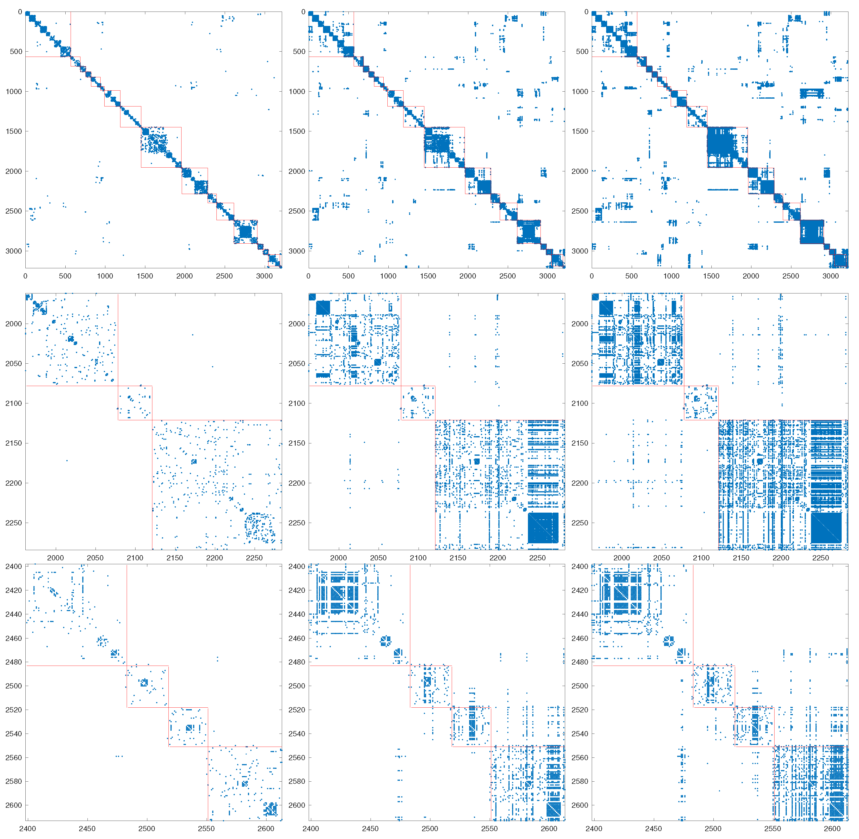
For our SAIR model, we suppose that the individuals in the A and I compartments may have different contact rates, denoted by β A and β I , and different recovery rates γ A and γ I , respectively. The meaning of these quantities is analogous to the SIR and SAIR models, that is, for X = A , I , β X X N indicates the probability of getting infected by having contact with an individual of the group X in a unit of time (day) and γ X = 1 T R , X , where T R , X is the mean infectious period for individuals in the group X.
We also consider a rate δ of individuals in A that may develop symptoms or are anyway detected and hence will move to the I compartment. This parameter depends also on the rapid detection of asymptomatic individuals [27].
Then, the constitutive equations of our SAIR model can be written as:
S = β A A + β I I N S , A = β A A + β I I N S ( γ A + δ ) A , I = γ I I + δ A , R = γ A A + γ I I ,
where now the total population is N = S + A + I + R .

2.2. Mobility Data

In this section we are going to describe in detail the mobility data between provinces and autonomous communities (CCAA) of Spain, provided by the INE, and explain how we used it in our model. The mobility data provided are based on the localization of cell phones. The data cover the three most important phone operators in Spain and they gather more than 80% of the cell phones in the country, so they can be considered realistic.
The study divided the national territory into 3214 mobility areas, which are population groups of between 5000 and 50,000 inhabitants (more homogeneous than the municipalities) and that can have totally different sizes. For instance, in rural areas where the population density is very low, a mobility area will be constituted by several municipalities, up to reach at least 5000 inhabitants, while deeply populated areas, like big cities as Madrid, are subdivided in several mobility areas of about 20,000 inhabitants on average.
From the start of the lockdown period (16 March 2020) up to the end of the state of alarm (22 June 2020), the information for each mobility area is provided, based on the analysis of 24 h periods. For the sake of comparison, mobility data for a reference day, that is, a typical working day before lockdown, was also provided as the average of the period 18–21 November 2019 (Monday to Thursday).
The data provided for each mobility area are:
  • The registered resident population (according to official records).
  • Number of individuals that stay at their area of residence.
  • Number of individuals that leave their area of residence, and number of cells receiving individuals from that cell.
  • The destination mobility areas to which those who leave their area go and the estimated number of people that move to them, with the restrictions indicated below due to privacy issues.
As indicated in Section 1, these mobility data are based on the localization of cell phones. They are based on the following assumptions:
  • A person is considered to reside in an area if their phone stays in said area from 0 a.m. to 6 a.m.
  • The destination area of that person, is the area where their mobile phone stays most of the time from 10 a.m. to 4 p.m., with a minimum of two hours. Hence, the destination area of a person can be their residence area, any other area, or none (if it does not stay more than two hours in the same area in the period considered).
  • The data is normalized with respect to the total population.
  • The phone operators that provided the data did not report flows of people smaller than 10 or 15 phones (depending on the phone company) in order to ensure privacy. Moreover, the estimated flow of people moving between each pair of areas is provided only if it is higher than 100 people. Smaller flows are not provided.
The last point raises the problem that there are mobility areas without information about where people have moved to. That means that if only these data are considered, these areas would appear as isolated areas, although we know that people have left and entered their residence area. Furthermore, if we merge some mobility areas to create a bigger area (such as a province or region) it might result in a loss of data, since one could have a bigger area with an estimated mobility much smaller than its real one.
With the aim of correcting this, and recovering the information of mobility between areas with an estimated mobility flux smaller than 100 people, we have proposed an algorithm that is explained in Section 2.6.

2.3. SAIR Model with Mobility

In this section we introduce the model proposed in this work for the analysis of the spread of infected individuals under mobility constraints. For this model, we divide the whole domain area into an arbitrary number of smaller spatial areas. In each spatial area, we use the SAIR model (3), and we add some terms to simulate the movement of people between regions.
Let us consider C N small spatial areas covering the whole original domain, and define variables S i , A i , I i , R i , for each area i = 1 , , C , and mobility fluxes m j k of individuals per day (which is taken as the unit of time) that move from area j to area k.
We assume that individuals in the I compartment do not move and that the mobility flux is a daily flux, that is, it is positive half a day and negative the other half, representing, for example, people going to work and back. This means that, at the first half of the day there are m j k individuals that move from area j to area k, i.e, from the compartments S j , A j , R j to the corresponding S k , A k , R k , while in the second half of the day the same amount of people go back to area j, but some of them have got infected during their stay at area k. If μ k denotes the probability of infection for individuals in the k-th compartment per day and taking into account that m j k S j S j + A j + R j susceptible individuals have traveled to area k and have been exposed to the disease for half a day in area k, then the number of individuals that got infected in the k compartment is given by
1 2 μ k m j k S j S j + A j + R j .
The factor 1 2 has been introduced because the time unit is a complete day and individuals stay just half a day in area k.
According to the SAIR model, the probability of getting infected for a susceptible individual in area j is given by
μ j = β A , j A j + β I , j I j N j ,
with N j = S j + A j + I j + R j . Hence, for each area j, the SAIR model without mobility (3) is given by
S j = μ j S j , A j = μ j S j ( γ A + δ ) A j , I j = γ I I j + δ A j , R j = γ A A j + γ I I j .
Note that different contact rates β A , j and β I , j have been considered for different areas, while the same values for γ A , γ I and δ are taken for all areas. This is motivated by the fact that the latter values are related to the evolution of the disease itself while the former depend on the behavior of the susceptible individuals, that may vary from area to area. Although there is no difficulty on considering different values for δ and/or γ in each area it would result on an unnecessary over-parameterization.
The susceptible individuals leaving area j in the first half of the day is given by
k m j k S j N j * ,
where N j * = S j + A j + R j = N j I j is the population in the j-th compartment that might move, while the ones entering area j in the same period are
k m k j S k N k * .
Hence, the flux of susceptible individuals in area j for the first half of the day, normalized for a unit time, is given by the term:
φ 1 ( t ) k m j k S j N j * m k j S k N k * ,
with the function φ 1 ( t ) defined by
φ 1 ( t ) = 2 , t t [ 0 , 1 / 2 ) , 0 , t t [ 1 / 2 , 1 ) ,
where the notation t stands for the floor function that gives the greatest integer smaller than or equal to t.
Still regarding the susceptible individuals, for the second half of the day we consider a similar term but subtracting the individuals that got infected during their stay at another area k, given by (4), that move to A k . Also, some individuals that came from area k to area j would move to A j . This results on a term
φ 2 ( t ) k m j k S j N j * 1 2 S j N j * μ k m k j S k N k * 1 2 S k N k * μ j ,
with
φ 2 ( t ) = 0 , t t [ 0 , 1 / 2 ) , 2 , t t [ 1 / 2 , 1 ) .
Therefore the evolution equation for susceptible individuals in compartment j gets the form
S j = μ j S j + φ 1 ( t ) k m j k S j N j * m k j S k N k * + φ 2 ( t ) k m j k S j N j * 1 2 S j N j * μ k m k j S k N k * 1 2 S k N k * μ j .
By a similar argument the evolution equation for the A j compartments is given by
A j = μ j S j ( γ A + δ ) A j + φ 1 ( t ) k m j k A j N j * m k j A k N k * + φ 2 ( t ) k m j k A j N j * + 1 2 S j N j * μ k m k j A k N k * + 1 2 S k N k * μ j ,
and for the R j compartment by
R j = γ A A j + γ I I j + φ 1 ( t ) k m j k R j N j * m k j R k N k * + φ 2 ( t ) k m j k R j N j * m k j R k N k * ,
as individuals in this compartment cannot get infected nor infect others. Finally, the equation for I j does not depend on mobility as infected individuals do not travel by hypothesis.
Grouping terms the model can be written as a system of 4 C ODEs given by:
S j = μ j S j + φ ( t ) k m j k S j N j * m k j S k N k * 1 2 φ 2 ( t ) k m j k S j N j * μ k m k j S k N k * μ j , A j = μ j S j ( γ A + δ ) A j + φ ( t ) k m j k A j N j * m k j A k N k * + 1 2 φ 2 ( t ) k m j k S j N j * μ k m k j S k N k * μ j , I j = γ I I j + δ A j , R j = γ A A j + γ I I j + φ ( t ) k m j k R j N j * m k j R k N k * ,
where φ = φ 1 + φ 2 .
With this setup the system has C + 3 parameters. It follows that there are no permanent transfers of population between areas, since the addition of the four equations in (5) yields for each j = 1 , , C :
N j ( t ) = φ ( t ) k ( m j k m k j ) ,
whose solution is
N j ( T ) = N j ( 0 ) + k ( m j k m k j ) 0 T φ ( t ) d t .
Therefore N j ( T ) = N j ( 0 ) whenever T N , since φ is 1-periodic and 0 1 φ ( t ) d t = 0 .
Also, note that according to the model, for n N
N j ( n + 1 2 ) = N j ( n ) + k ( m j k m k j ) n n + 1 2 φ ( t ) d t = N j ( 0 ) + k ( m k j m j k ) ,
that is, the model predicts that the individuals are one half of the day at their residence area, and the other half at their destination area.

2.4. SIR Model with Mobility

For the sake of comparison, we also consider the SIR model with mobility. In this case asymptomatic and non-asymptomatic infected individuals belong to the same group I j and they all are infectious. We assume that only a fraction ε of the individuals in I j (e.g., the asymptomatic ones, as individuals with symptoms will feel sick and stay at home) move from their area. The model is constructed in the same way as the SAIR model with mobility, taking into account that the compartments A j and I j are merged together and that the terms describing mobility for the infectious individuals are multiplied by ε . The model can be written as a system of 3 C ODE:
S j = μ j S j + φ 1 ( t ) k m j k S j N j * m k j S k N k * + φ 2 ( t ) k m j k S j N j * 1 2 S j N j * μ k m k j S k N k * 1 2 S k N k * μ j , I j = μ j S j γ I j + ε φ 1 ( t ) k m j k I j N j * m k j I k N k * + ε φ 2 ( t ) k m j k I j N j * m k j I k N k * + 1 2 φ 2 ( t ) k S j N j * μ k + S k N k * μ j , R j = γ I j + ( φ 1 ( t ) + φ 2 ( t ) ) k m j k R j N j * m k j R k N k * ,
where now N j * = S j + ε I j + R j is the population in the j-th compartment that might move and
μ j = β j I j N j .
Also in this case there are no permanent transfers of population between compartments, by the same reasoning as in the SAIR model with mobility.

2.5. Variable Parameters in the Compartmental Models

The contact rates ( β in the SIR model (1), β A and β I in the SAIR model (3)) are often taken as constants. This choice may be reasonable for cases where no prophylactic measures are taken to stop the infection spread (for example, seasonal influenza). In the case of the COVID-19 in Spain, various measures have been taken in different phases of the pandemic evolution, to try to dramatically reduce its spread first by a severe confinement on 15 March 2020, and later to recover some economic activity, by means of a 4-phase de-escalation plan, started on 2 May 2020 and finished on 22 June 2020. Each phase consisted on different contention policies.
To model the different stages of the lockdown and de-escalation period regarding mobility restrictions and their effect on the contact rates of the infection, we propose to consider discontinuous functions for the contact rates:
β j ( t ) = β j , 1 t t j , 1 β j , 2 t j , 1 < t t j , 2 , 0 < t j , 1 < ,
with β j , 1 , β j , 2 , given positive numbers and the times t j , 1 , t j , 2 , chosen appropriately. The same can be done for the parameters β A , j and β I , j in the SAIR model.
To account for changes in the mobility patterns, there is the possibility of changing the mobility terms φ i ( t ) m j , k , i = 1 , 2 , by φ i ( t ) m j , k , t , where m j , k , l is the flux between cells j and k on the l-th day.
Finally, taking into consideration the advances in the medical treatment of the disease, a time-varying function γ ( t ) could also be considered to model different recovery rates throughout the pandemic evolution in the same fashion we have done with the function β ( t ) . This can also be extended for the parameters γ A and γ I in the SAIR model, but it is beyond the scope of this paper.
Although these functions would yield a discontinuous right hand for the system of ODEs, the theory of discontinuous ODEs covers these cases [28], so that there is a unique continuous solution, with discontinuous lateral derivatives at the jumps of the coefficients.

2.6. Completing Fluxes

As mentioned in Section 2.2, in order to estimate the possible missing data when merging mobility areas, we aim to use the information provided as, for instance, the daily sum of all the outgoing fluxes and the number of receiving cells from each source cell.
Let N j be the population of cell j, d j , k the distance between the centroids of the cells j and k, and g j , k = N k / max ( d j , k , ε ) , for some ε > 0 (which we take as 10 5 in our experiments). The coordinates of the centroids are the average of the coordinates of the towns in the cell weighted by their population. For the source cell j, we denote by n j the number of cells receiving individuals from cell j and by f j the number of individuals leaving cell j on a given date. The provided fluxes, obtained from real data, between cells j and k are denoted by m j k * . We recall that, as indicated in Section 2.2, these are the fluxes between areas that are higer than 100 people.
Our goal is to define fluxes m j k between cells j and k such that:
  • If m j k * 0 m j k = m j k * ( m j k “complete” the provided fluxes)
  • | { k / m j k 0 } | = n j , k m j k = f j (match the global information of outgoing fluxes).
The strategy is to assign the non-assigned f ˜ j = f j k m j k * individuals issuing from cell j to the first n ˜ j = n j | { k / m j k * 0 } | cells in a descending ranking according to g j , k :
g j , k 1 g j , k 2 g j , k n ˜ j , m j k = f ˜ j g j , k l s = 1 n ˜ j g j , k s , if k = k l , l = 1 , , n ˜ j , 0 , otherwise .

3. Numerical Experiments and Validation

In this section we validate the model presented in Section 2.3 in various scenarios. In Section 3.1 we study how the mobility data and the way in which missing data is completed affects the simulation results. In Section 3.2 we try to simulate a real outbreak corresponding to the region of A Mariña in Spain.

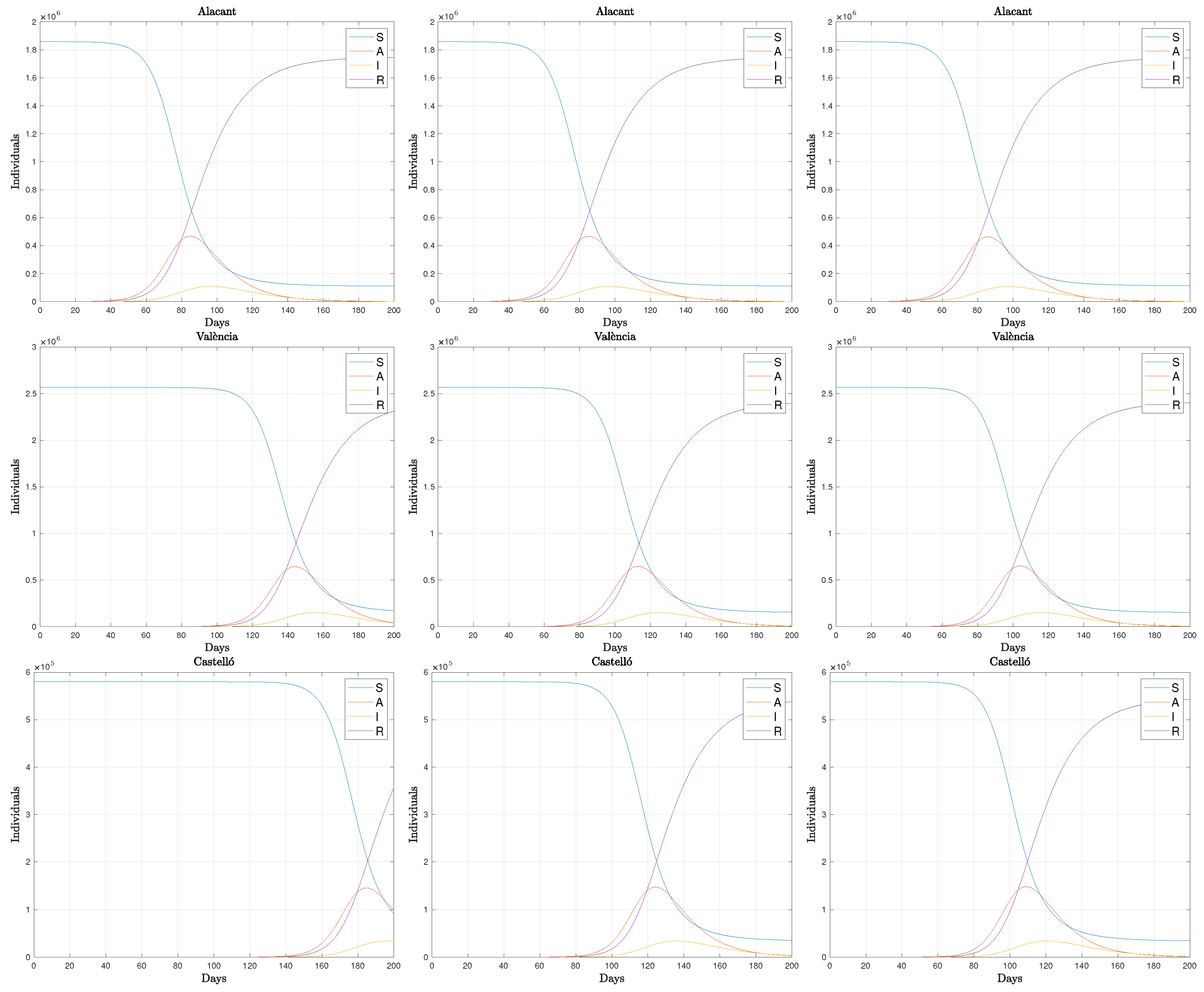
3.1. How Mobility Affects the Spread of Covid-19

In this section we analyze various types of mobility data. In particular three types of mobility are considered:
  • Very restricted mobility: we define the mobility fluxes using the INE data from April 1.
  • Restricted mobility: the mobility fluxes are obtained with the algorithm in Section 2.6 from the INE data of April 1.
  • Unrestricted mobility: in this case, the mobility fluxes are obtained with the algorithm in Section 2.6 but from the INE November reference data.
In Figure 1 the mobility flow matrices for Spain (first row) and for the autonomous communities of Galicia and Valencia, second and third row respectively, can be seen. In the first column we have the movements based on the INE data of April 1 (very restricted mobility) while in the second and third columns the results obtained with the algorithm in Section 2.6 using the INE data of 1 April and November (restricted mobility and unrestricted mobility) respectively, are shown. We only show the movements between areas when there are more than 10 people moving between them, although in the experiments we consider all the movements obtained. In the top row the red squares correspond to autonomous regions, while in the second row they correspond to the provinces in the Valencia region (Alacant, Castelló and Valencia) and in the last row they correspond to the provinces in Galicia (A Coruña, Lugo, Ourense and Pontevedra).
Now we consider some experiments in autonomous communities that we suppose completely isolated from the outside. In these experiments we have set the parameters γ A = γ I = 1 / 15 , constant in all areas, δ = 1 / 50 and β = 3 γ . These values have been set according to estimations of the incubation and infectious periods of the disease [29,30], with a slightly high incubation period to make the effect more evident and stand for the time required for the incorporation of individuals to official records. The value of β corresponds to a basic reproduction number R 0 = 3 . For the numerical solution of the model we have used the MATLAB ODE package.
First we consider the Valencian Autonomous Community. We assume that Alicante has 40 asymptomatic infectious individuals and the other two provinces have none. We see in Figure 2 how the development of COVID-19 is different when the different types of mobility are considered.
As a second example, we consider the Autonomous Community of Galicia, where we separate A Mariña from the rest of Lugo province. We assume that A Mariña has 40 asymptomatic infectious individuals and the rest of the provinces have none. In Figure 3 we see the results obtained.
In both Figure 2 and Figure 3 it can be seen that COVID-19 spreads more quickly to closer areas, and that if mobility is less restricted, it appears earlier. In Figure 3 it can be seen that when using very restricted mobility fluxes, COVID-19 does not reach the rest of Lugo province and it is because with these mobility fluxes it is completely isolated from A Mariña and the rest of the provinces.
In these experiments we are considering mobility restrictions between regions or provinces but not within them. This is why the behavior in the regions where infected individuals are initially located (Alacant or A Mariña) is the same independently of the mobility restrictions considered. A finer look to the influence inside each region could be done by considering all mobility areas of the Autonomous Communities (217 in Galicia, 324 in Valencia), but information regarding the number of infected individuals was not given with such detail by the INE. Also, variable parameters in the SAIR model, depending on mobility restrictions, can be considered, as has been done in the experiment of Section 3.2.

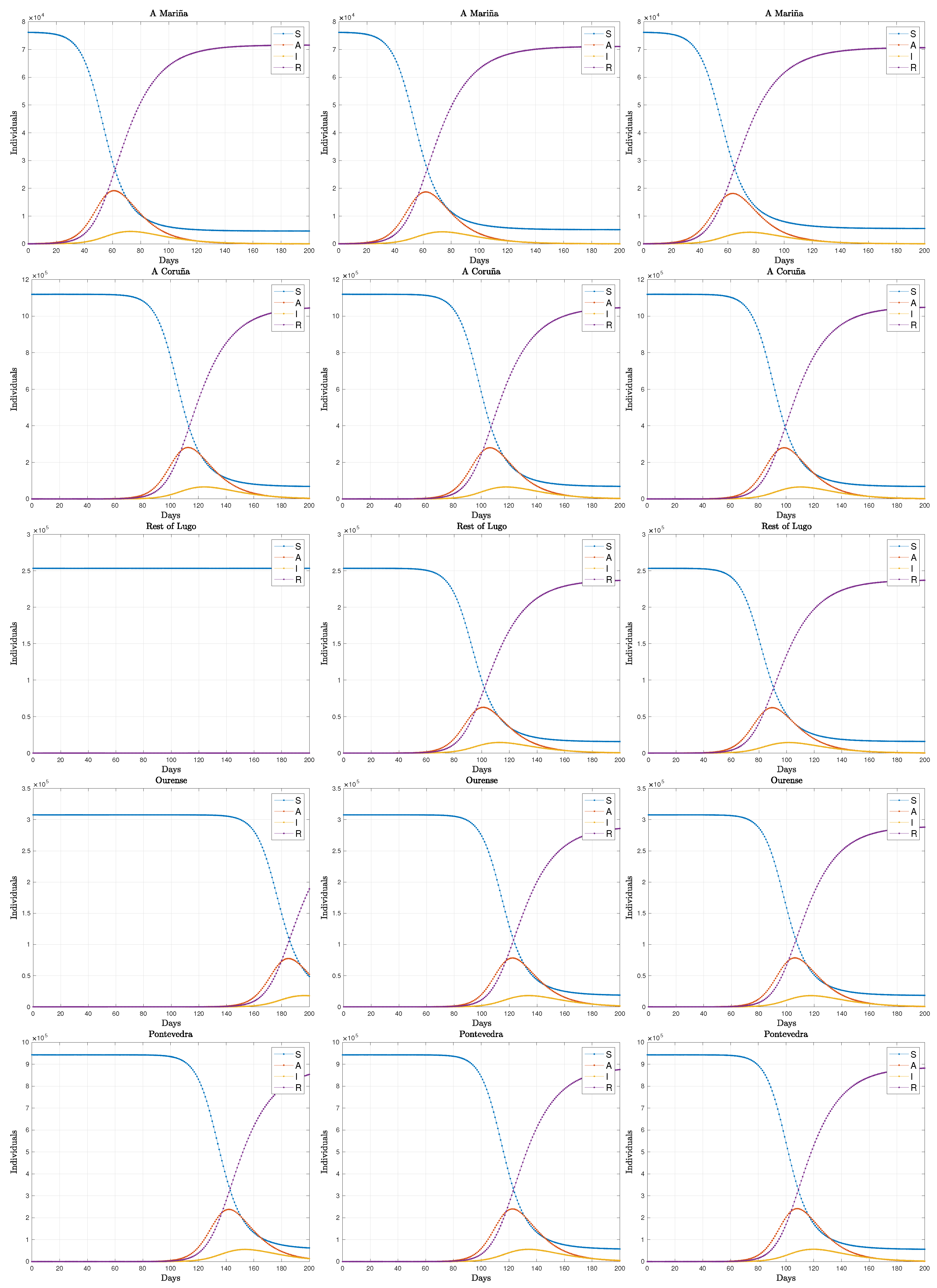
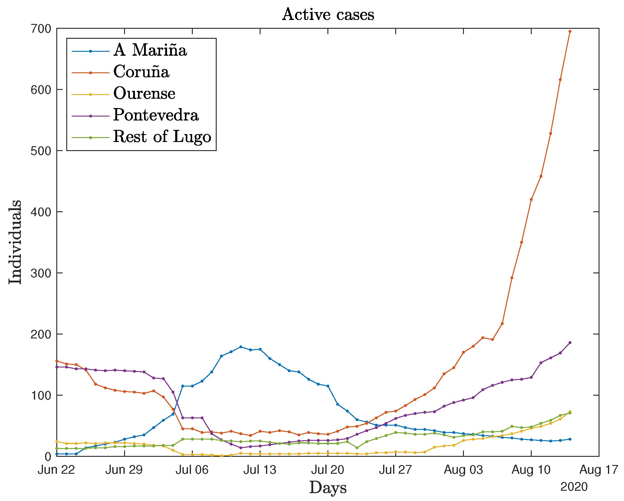
3.2. Outbreak in the A Mariña Area, Galicia, Spain

A Mariña is an area located in the northern part of the province of Lugo, in the autonomous region of Galicia, at the northwest of Spain. It has an extension of about 1650 Km 2 and a population of nearly 70,000 people. On 6 July 2020, an outbreak of COVID-19 was declared in that area and mobility restrictions as well as other control measures were dictated so that trips within the area were allowed but limitations were imposed for trips from or to the outside of the area. The lockdown measures were progressively retired, depending on the particular village, up to 22 July 2020, when mobility was again free. Let us summarize the timeline of the outbreak:
  • 22 June 2020: End of the state of alarm in Spain. Mobility restrictions do not apply anymore.
  • 23 June 2020: A new case is detected in the village of Xove, in the Galician region, A Mariña area.
  • 5 July 2020: 106 new cases had been detected in the area since 23 June 2020.
  • 6 July 2020: Lockdown is dictated for the area of A Mariña. Restrictions apply for the municipalities of Alfoz, Barreiros, Burela, Cervo, Foz, Lourenzá, Mondoñedo, Ourol, Ribadeo, Trabada, O Valadouro, O Vicedo, Viveiro and Xove.
  • 12 July 2020: Mobility restrictions were retired for some municipalities.
  • 22 July 2020: Mobility restrictions were retired for the full area of A Mariña.
  • 20 August 2020: The regional government declared that the A Mariña outbreak is controlled.
Figure 4 shows the official active cases as reported by the authorities [31]. The outbreak in the A Mariña area achieved its maximum on 11 July 2020 and spread to the rest of Galicia. The incidence outside A Mariña due to the spread of the outbreak cannot be split from the rest of the cases, due to other imported cases or to local contacts but the effect of the outbreak in other territories seems evident.
In this subsection we test to what extent our model can simulate such an outbreak. Let us clarify that we do not intend to exactly predict the outbreak figures but to analyze the effects of the various parts of the model and to what extent they can qualitatively represent the outbreak tendencies. This is due to the fact that the data provided by the authorities do not accurately represent the real incidence of the epidemic, because of many factors: undetected cases, unknown number of asymptomatic individuals, different criteria for case reporting among the different autonomous regions, and so forth.
Figure 5 shows the result of various simulations regarding this outbreak. The Galician region has been split into five parts: A Mariña, the complete provinces of Coruña, Ourense and Pontevedra, and the rest of the province of Lugo. The plots show infected individuals, counting for the sum of infected and asymptomatic in the case of the SAIR model. The results have been obtained using the initial data given by 1000 asymptomatic individuals and 100 infected in A Mariña and zero at the rest, in order to take apart the effect of the outbreak from other effects. These data come from the fact that, according to Reference [26], the prevalence of COVID-19 in Spain is about 10 times higher than the reported cases and on the other hand there is a delay in the process of including data in the official records. In any case, as mentioned, the data does not intend to represent real figures, but tendencies. Let us also mention that the rescaling of the initial data produces results that are not in the same scale as the real reported data. The results have thus been rescaled back so that the numbers shown in Figure 5 are put on a scale similar to the ones in Figure 4. We have set the parameters δ = 1 / 25 , γ A , I = 1 / 15 , based on estimations of the incubation and infectious periods of the disease [29,30]. The values for the contact rates have been taken as β A = 5 γ and β I = 6 γ in all regions. These correspond to basic reproduction numbers R 0 , A = β A γ A = 5 and R 0 , I = β I γ I = 6 , which may be valid numbers only on the onset of the epidemics. Our present aim is to assess the capability of the model of triggering an outbreak in a location without initial infectious individuals.
In the cases where a reduction of the contact rates is indicated, the above values are reduced by a factor of 2, only in the area of A Mariña. The mobility fluxes have always been completed according to the algorithm described in Section 2.6.
The top left plot in Figure 5 tries to reproduce the real situation in which a lockdown is imposed from 6 July 2020 to 22 July 2020 (days 14–30). The contact rates β A and β I have been also reduced in that period, representing the mild official recommendation (not mandatory) of leaving one’s house only if necessary. The figure shows that the outbreak effectively spreads to the rest of the areas. The model shows a peak value of infections at the beginning of August that does not appear in the real data, but this can be due to the rescaling of the data, to the influence of factors different from the outbreak itself or to a limitation of the model.
The top right plot in Figure 5 corresponds to the situation where the contact rates β A and β I are not reduced during the lockdown period. As can be seen, the results are very similar, indicating that in this case a mild reduction on the social contact does not have a big impact on the evolution of the outbreak.
The second row in Figure 5 corresponds to the case where no mobility restrictions are applied. In these plots the mobility fluxes have been set to the ones of a normal day before lockdown taken as reference. It can be seen that either with a reduction on the contact rates during days 14–30 (left plot) or without it (right plot) the outbreak spreads faster to the rest of the territories than if restrictions are applied. Also, the peak values of infections are slightly higher.
For comparison, in the last row we show a result obtained with the SIR model including mobility. The left plot corresponds to restricted mobility fluxes, and the right plot to unrestricted fluxes, with constant contact rates. The value ε that appears in the model has been set to 0.9 , being all other values set to the same values as in the SAIR model. It can be observed that the model also predicts the spread of the disease to the neighboring regions in a way similar to the SAIR model, but with the need of tuning the parameter ε . Note that in this case the maximum values for infections are slightly smaller, due to a different parameter tuning.

4. Conclusions

In this paper, we present a mathematical model for the simulation of the spread of small epidemic outbreaks. The model is based on the division of a region into smaller areas, called mobility areas, for which mobility fluxes are known, and describe the evolution of an outbreak in one of the pieces by a model which combines a deterministic SAIR compartmental model and terms that include the effects of people’s mobility among areas. The model includes also limited capabilities for the modeling of social confinement measures. As mobility data are sometimes incomplete, we also describe a method for the completion and homogenization of fluxes. Numerical results show that the model is able to qualitatively represent the tendencies of small outbreaks.

Author Contributions

Data curation, F.A. and P.M.; funding acquisition, P.M.; investigation, F.A., A.B., I.C.-C., R.D., M.C.M., P.M. and D.F.Y.; methodology, A.B. and P.M.; software, F.A., A.B. and P.M.; supervision, A.B.; Visualization, F.A.; writing—original draft, F.A., A.B., I.C.-C. and P.M.; writing—review & editing, A.B., M.C.M. and D.F.Y. All authors have read and agreed to the published version of the manuscript.

Funding

This research was funded by Spanish MINECO project MTM2017-83942-P, by Spanish Agencia Estatal de Investigacóin Grant No. PGC2018-095984-B-I0, by Generalitat Valenciana Grant. No. PROMETEO/2019/071 and by European Cooperation in Science and Technology (COST) Grant. No. COST Action CA17137.

Conflicts of Interest

The authors declare no conflict of interest. The funders had no role in the design of the study; in the collection, analyses, or interpretation of data; in the writing of the manuscript, or in the decision to publish the results.

Nomenclature (Units Are Indicated in Brackets)

Latin symbols
AAsymptomatic individuals [ individuals ]
A j Asymptomatic individuals of area j [ individuals ]
d j , k Distance between the centroids of the j-th and k-th cells [ km ]
EExposed individuals [ individuals ]
f j Individuals leaving cell j on a given day [ individuals ]
g j , k Quantity used in the algorithm for flux completion [ individuals · km 1 ]
IInfectious individuals [ individuals ]
I j Infectious individuals of area j [ individuals ]
m j , k Mobility flux from area j to area k [ individuals · day 1 ]
m j , k * Mobility flux from area j to area k provided by real data [ individuals · day 1 ]
m j , k , l Mobility flux from area j to area k on the l-th day [ individuals · day 1 ]
n j Number of cells that receive individuals from cell j [ cells ]
NTotal population [ individuals ]
N j Total population of area j [ individuals ]
N j * Population in the j-th compartment that might move [ individuals ]
RRetired individuals [ individuals ]
R j Retired individuals of area j [ individuals ]
R 0 Basic reproduction number [ - ]
SSusceptible individuals [ individuals ]
S j Susceptible individuals of area j [ individuals ]
T I Mean incubation period [ days ]
T R Mean infectious period [ days ]
T R , j Mean infectious period for individuals in the j compartment [ days ]
Greek symbols
β j Contact rate of compartment j [ days 1 ]
β j , k Contact rate of compartment j and area k [ days 1 ]
γ j Recovery rate of compartment j [ days 1 ]
γ j , k Recovery rate of compartment j and area k [ days 1 ]
δ Rate of asymptomatic individuals that may develop symptoms [ days 1 ]
ε Fraction of individuals in the I compartment of the SIR model moving from their area [ - ]
η Incubation rate [ days 1 ]
μ j Probability of getting infected for a susceptible individual in area j [ - ]
φ 1 ( t ) Auxiliary function used to define the flux of individuals in area j for the first half of the day [ - ]
φ 2 ( t ) Auxiliary function used to define the flux of individuals in area j for the second half of the day [ - ]

References

  1. Bürger, R.; Chowell, G.; Mulet, P.; Villada, L.M. Modelling the spatial-temporal progression of the 2009 A/H1N1 influenza pandemic in Chile. Math. Biosci. Eng. 2016, 13, 43–65. [Google Scholar] [CrossRef] [PubMed]
  2. Brauer, F.; Castillo-Chávez, C. Mathematical Models in Population Biology and Epidemiology, 2nd ed.; Springer: Berlin/Heidelberg, Germany, 2012. [Google Scholar]
  3. Diekmann, O.; Heesterbeek, H.; Britton, T. Mathematical Tools for Understanding Infectious Disease Dynamics; Princeton University Press: Princeton, NJ, USA, 2013. [Google Scholar]
  4. Weiss, H. The SIR model and the foundations of public health. Mater. Math. 2013, 3, 17. [Google Scholar]
  5. Allen, L.J.S. A primer on stochastic epidemic models: Formulation, numerical simulation, and analysis. Infect. Dis. Model. 2017, 2, 128–142. [Google Scholar] [CrossRef] [PubMed]
  6. Kermack, W.O.; McKendrick, A.G. A contribution to the mathematical theory of epidemics. Proc. R. Soc. A 1927, 115, 700–721. [Google Scholar] [CrossRef] [Green Version]
  7. Chowell, G. Fitting dynamic models to epidemic outbreaks with quantified uncertainty: A primer for parameter uncertainty, identifiability, and forecast. Infect. Dis. Model. 2017, 2, 379–398. [Google Scholar] [CrossRef]
  8. Barlow, N.S.; Weinstein, S.J. Accurate closed-form solution of the SIR epidemic model. Phys. D Nonlinear Phenom. 2020, 408, 132540. [Google Scholar] [CrossRef]
  9. Weinstein, S.J.; Holland, M.S.; Rogers, K.E.; Barlow, N.S. Analytic solution of the SEIR epidemic model via asymptotic approximant. Phys. D Nonlinear Phenom. 2020, 411, 132633. [Google Scholar] [CrossRef]
  10. Wu, J.T.; Leung, K.; Leung, G.M. Nowcasting and forecasting the potential domestic and international spread of the 2019-nCoV outbreak originating in Wuhan, China: A modelling study. Lancet 2020, 395, 689–697. [Google Scholar] [CrossRef] [Green Version]
  11. Tang, B.; Wang, X.; Li, Q.; Bragazzi, N.L.; Tang, S.; Xiao, Y.; Wu, J. Estimation of the Transmission Risk of the 2019-nCoV and Its Implication for Public Health Interventions. J. Clin. Med. 2020, 9, 462. [Google Scholar] [CrossRef] [Green Version]
  12. He, S.; Peng, Y.; Sun, K. SEIR modeling of the COVID-19 and its dynamics. Nonlinear Dyn. 2020. [Google Scholar] [CrossRef]
  13. Giordano, G.; Blanchini, F.; Bruno, R.; Colaneri, P.; Filippo, A.D.; Matteo, A.D.; Colaneri, M. Modelling the COVID-19 epidemic and implementation of population-wide interventions in Italy. Nat. Med. 2020, 26, 855–860. [Google Scholar] [CrossRef] [PubMed]
  14. Arcede, J.P.; Caga-anan, R.L.; Mentuda, C.Q.; Mammeri, Y. Accounting for symptomatic and asymptomatic in a SEIR-type model of COVID-19. Math. Model. Nat. Phenom. 2020, 15, 1–11. [Google Scholar] [CrossRef]
  15. Alleman, T.W.; Vergeynst, J.; Torfs, E.; Gonzalez, D.I.; Nopens, I.; Baetensand, J.M. A deterministic, age-stratified, extended SEIRD model for assessing the effect of non-pharmaceutical interventions on SARS-CoV-2 spread in Belgium. medRxiv 2020. [Google Scholar] [CrossRef]
  16. Lyra, W.; do Nascimento, J., Jr.; Belkhiria, J.; de Almeida, L.; Chrispim, P.P.M.; de Andrade, I. COVID-19 pandemics modeling with SEIR(+CAQH), social distancing, and age stratification. The effect of vertical confinement and release in Brazil. medRxiv 2020. [Google Scholar] [CrossRef] [Green Version]
  17. Peixoto, P.S.; Marcondes, D.; Peixoto, C.; Oliva, S.M. Modeling future spread of infections via mobile geolocation data and population dynamics. An application to COVID-19 in Brazil. PLoS ONE 2020, 15, e0235732. [Google Scholar] [CrossRef]
  18. Arenas, A.; Cota, W.; Gomez-Gardenes, J.; Gómez, S.; Granell, C.; Matamalas, J.T.; Soriano-Panos, D.; Steineggerand, B. A mathematical model for the spatiotemporal epidemic spreading of COVID19. medRxiv 2020. [Google Scholar] [CrossRef] [Green Version]
  19. Robinson, M.; Stilianakis, N.I. A model for the emergence of drug resistance in the presence of asymptomatic infections. Math. Biosci. 2013, 243, 163–177. [Google Scholar] [CrossRef]
  20. Grunnill, M. An exploration of the role of asymptomatic infections in the epidemiology of dengue viruses through susceptible, asymptomatic, infected and recovered (SAIR) models. J. Theor. Biol. 2018, 439, 195–204. [Google Scholar] [CrossRef]
  21. Liu, C.; Wu, X.; Niu, R.; Wu, X.; Fan, R. A new SAIR model on complex networks for analysing the 2019 novel coronavirus (COVID-19). Nonlinear Dyn. 2020. [Google Scholar] [CrossRef]
  22. Monteiro, L. An epidemiological model for SARS-CoV-2. Ecol. Complex. 2020, 43, 100836. [Google Scholar] [CrossRef]
  23. Day, M. Covid-19: Four fifths of cases are asymptomatic, China figures indicate. BMJ 2020, 369. [Google Scholar] [CrossRef] [Green Version]
  24. Mizumoto, K.; Kagaya, K.; Zarebski, A.; Chowell, G. Estimating the asymptomatic proportion of coronavirus disease 2019 (COVID-19) cases on board the Diamond Princess cruise ship, Yokohama, Japan, 2020. Euro Surveill 2020, 25, 2000180. [Google Scholar] [CrossRef] [PubMed] [Green Version]
  25. Nishiura, H.; Miyama, T.; Suzuki, A.; Jung, S.M.; Hayashi, K.; Kinoshita, R.; Yang, Y.; Yuan, B.; Akhmetzhanov, A.R.; Linton, N.M. Estimation of the asymptomatic ratio of novel coronavirus infections (COVID-19). Int. J. Infect. Dis. 2020, 94, 154–155. [Google Scholar] [CrossRef]
  26. Pollán, M.; Pérez-Gómez, B.; Roberto Pastor-Barriuso, R.; Oteo, J.; Hernán, M.A.; Pérez-Olmeda, M.; Sanmartín, J.L.; Fernández-García, A.; Cruz, I.; Fernández de Larrea, N.; et al. Prevalence of SARS-CoV-2 in Spain (ENE-COVID): A nationwide, population-based seroepidemiological study. Lancet 2020. [Google Scholar] [CrossRef]
  27. Nguyen, T.; Bang, D.D.; Wolff, A. 2019 Novel Coronavirus Disease (COVID-19): Paving the Road for Rapid Detection and Point-of-Care Diagnostics. Micromachines 2020, 11, 306. [Google Scholar] [CrossRef] [PubMed] [Green Version]
  28. Filippov, A.F. Differential Equations with Discontinuous Righthand Sides; Mathematics and Its Applications (Soviet Series); Kluwer Academic Publishers Group: Dordrecht, The Netherlands, 1988; Volume 18. [Google Scholar] [CrossRef]
  29. Lauer, S.A.; Grantz, K.H.; Bi, Q.; Jones, F.K.; Zheng, Q.; Meredith, H.R.; Azman, A.S.; Reich, N.G.; Lessler, J. The Incubation Period of Coronavirus Disease 2019 (COVID-19) From Publicly Reported Confirmed Cases: Estimation and Application. Ann. Int. Med. 2020, 172. [Google Scholar] [CrossRef] [Green Version]
  30. Wölfel, R.; Corman, V.M.; Guggemos, W.; Seilmaier, M.; Zange, S.; Müller, M.A.; Niemeyer, D.; Jones, T.C.; Vollmar, P.; Rothe, C.; et al. Virological assessment of hospitalized patients with COVID-2019. Nature 2020, 581, 465–469. [Google Scholar] [CrossRef] [PubMed] [Green Version]
  31. COVID-19 Page of the Instituto de Salud Carlos III. Available online: https://cnecovid.isciii.es/covid19 (accessed on 25 September 2020).
Figure 1. From top to bottom: movements between the 3214 mobility areas organized alphabetically by Autonomous Communities, between the areas of the provinces of Valencia and between the areas of the provinces of Galicia. From left to right: movements between areas of more than 100 people (Spanish National Institute of Statistics (INE) data 1 April), movements between areas obtained with our algorithm from the INE data of April 1 and from the INE data of November. In the two last cases the fluxes are only shown when more than 10 people have moved between areas.
Mathematics 08 01677 g001
Figure 2. Simulation of the evolution of COVID-19 in the different provinces of the Valencian Autonomous Community, assuming that initially Alacant has 40 asymptomatic infectious individuals and Castelló and València have none, and considering different mobility restrictions between provinces. From left to rigth: very resticted mobility, restricted mobility and unrestricted mobility.
Mathematics 08 01677 g002
Figure 3. Simulation of the evolution of COVID-19 in five regions of the Autonomous Community of Galicia assuming that initially A Mariña has 40 asymptomatic infectious individuals and A Coruña, rest of Lugo (Lugo without A Mariña), Ourense and Pontevedra have none, and considering different mobility restrictions among the five regions. From left to rigth: very resticted mobility, restricted mobility and unrestricted mobility.
Mathematics 08 01677 g003
Figure 4. Active cases in the A Mariña area, Spain.
Mathematics 08 01677 g004
Figure 5. Predicted active cases (A+I) for different simulations of the A Mariña outbreak. From left to right and from top to bottom: SAIR, with mobility restrictions and reduced contact rates applied on days 14–30; Same experiment with constant contact rates; SAIR, without mobility restrictions and reduced contact rates applied on days 14–30; SIR with restricted mobility on days 14–30; SIR with unrestricted mobility on days 14–30.
Mathematics 08 01677 g005

