Fractional-Order SIR Epidemic Model for Transmission Prediction of COVID-19 Disease


Department of Electrical, Control and Computer Engineering, Opole University of Technology, 45-758 Opole, Poland
*
Author to whom correspondence should be addressed.
Appl. Sci. 2020, 10(23), 8316; https://doi.org/10.3390/app10238316
Submission received: 20 October 2020
/
Revised: 17 November 2020
/
Accepted: 18 November 2020
/
Published: 24 November 2020
(This article belongs to the Special Issue Fighting COVID-19: Emerging Techniques and Aid Systems for Prevention, Forecasting and Diagnosis)
Abstract
:In this paper, the fractional-order generalization of the susceptible-infected-recovered (SIR) epidemic model for predicting the spread of the COVID-19 disease is presented. The time-domain model implementation is based on the fixed-step method using the nabla fractional-order difference defined by Grünwald-Letnikov formula. We study the influence of fractional order values on the dynamic properties of the proposed fractional-order SIR model. In modeling the COVID-19 transmission, the model’s parameters are estimated while using the genetic algorithm. The model prediction results for the spread of COVID-19 in Italy and Spain confirm the usefulness of the introduced methodology.
1. Introduction
Coronavirus disease 2019 (COVID-19) is an acute infectious disease of the respiratory system that is caused by the SARS-CoV-2 virus infection. The World Health Organization (WHO) issued the official name and explained it as CO for corona, VI for virus, D for disease, and 19 for the year of first identification. The infection symptoms are usually a fever, dry cough, fatigue, loss of appetite, and shortness of breath. COVID-19 was first recognized and described on December 8, 2019, in the Wuhan, Republic of China. As a result of rapidly spreading the virus into other countries and continents, on March 11, 2020, WHO classified COVID-19 as a pandemic. With both mortality and infectiousness rates, COVID-19 is recognized as the worst pandemic in modern times since the flu pandemic of the early 20th century.
Mathematical modeling theories of infectious disease transmission dynamics have prompted considerable research interest, as the worldwide issue of the COVID-19 outbreak has attracted scientists from different areas [1,2,3]. The Susceptible-Infected-Removed (SIR) epidemic model is a classical compartmental model that is widely used to predict the progress of infectious disease [4,5,6]. Its origins date to the fundamental work by Kermack and McKendrick in the early 20th century [7].
Although the SIR model may be useful in modeling several epidemic processes, it may not be sufficient to describe the COVID-19 spread dynamics. Therefore, there are some modifications to the SIR model used in the approximation of COVID-19 disease [8]. Kucharski et al. [9] used the SEIR (susceptible-exposed-infectious-removed) compartment model in order to study the transmission and control of COVID-19. Sarkar et al. [10] proposed an SEIR model extended by adding contact tracing and other interventions, such as quarantine, lockdown, and social distancing. The SIDARTHE (susceptible-infected-diagnosed-ailing-recognized-threatened-healed-extinct) model with differentiating between diagnosed and non-diagnosed individuals has been presented by Giordano et al. [11] in order to analyze the COVID-19 epidemic in Italy. In [12], Ndaïrou et al. introduced the SEIPAHRF (susceptible-exposed-symptomatic infectious-super spreaders-asymptomatic infectious-hospitalized-recovered-fatality) model that considers the class of super-spreaders in order to study the transmission dynamics for the outbreak that occurred in Wuhan, China.
On the other hand, it is well known that the implementation of fractional calculus in differential equations of various processes, which lead to fractional-order generalizations of the modeling approaches, can significantly improve the modeling performance in several processes. Hence, many scientists have paid attention to this mathematical analysis branch, as it may give a better understanding of some complex physical phenomena, where ordinary calculus fails to provide a precise explanation. Atangana and Gómez-Aguilar [13] applied fractional derivative to model chaos and statistics. Ghanbari and Atangana [14] used the Atangana—Baleanu definition for the fractional derivative to introduce the new fractional mask for image denoising. Morales-Delgado et al. [15] obtained solutions of a cancer chemotherapy effect model involving the Caputo-Fabrizio and Atanagana-Baleanu fractional derivatives. There are some papers considering the fractional-order derivate implemented in the compartment models. A fractional-order extended SEIR (susceptible-exposed-infectious-removed) model considering interaction among people and the reservoir of the infection (seafood market) has been presented and studied by Khan and Atangana [16]. Srivastava and Gerhan [17] used the conformable fractional differential transform method to compute an approximate solution of the fractional-order SIR epidemic model of childhood disease. Abdo et al. [18] presented a nonlinear fractional-order model under the fractional Adam-BashForth method. In this work, we will implement the Grünwald-Letnikov fractional-order derivative into the classical SIR model in order to simulate and predict the COVID-19 outbreak.
The paper is organized, as follows. Having introduced the problem of modeling the COVID-19 transmission in Section 1, Section 2 presents the ’classical’ SIR model. The fractional-order generalization of the SIR model and its fixed-step implementation are introduced in Section 3. Section 4 presents the influence of fractional orders on model dynamical properties and presents virus transmission modeling in Spain and Italy. The conclusions of Section 5 complete the paper.
2. Preliminaries
The SIR model is one of the simplest compartment models, and many others are derivatives of its basic form. The total population N is divided into three epidemiological subpopulations: The number of susceptible individuals. When a susceptible and an infectious person come into contact, the susceptible individual contracts the disease and transitions to the infectious compartment, The number of infectious individuals. These individuals have been infected and they can infect susceptible individuals, , the number of removed individuals. This subpopulation consists of individuals who are immune due to natural immunity, have recovered from the disease and gained immunity, or have died. The SIR model consists of three ordinary differential equations that are presented below.
where and are infection and recovery rate, respectively.
Birth and death dynamics are usually neglected in simple compartmental models, since the dynamics of an epidemic, such as the flu, are often much faster than the dynamics of birth and death, and the numerical simulations are often executed for short time intervals.
Note that the dynamics of infectious disease depends on the following ratio:
where is the basic reproduction number. This ratio quantifies the expected number of cases that are directly generated by one individual in an infected population. When , the infection will be able to start spreading, causing a potential outbreak. If the disease will cease to exists.
3. Fractional-Order Generalization of SIR Model
It is well known that the integer-order derivative can be generalized by the fractional-order counterpart. In this case, the derivative is presented in the form of , where the order . Note that the derivative is usually defined in one of three definitions, e.g., Caputo, Rieman-Liouville, and Grünwald-Letnikov ones. In the paper, Grünwald-Letnikov [19] is exploited hereinafter, where
with t is continuous-time, h is sampling interval and denoting newton binomial, which (for ) can be calculated using the Pochhammer function as
In application, we use fixed step method, where we use nabla difference defined in discrete-time , such that . The nabla difference is defined as
Note that, for satisfactory low h, we have , so that we can effectively use the discrete-time difference to model continuous time processes.
It is well known that the incorporation of fractional-order derivative into model equations can lead to improving model parameters in several physical processes. In particular, various diffusion processes can be better modeled by use of fractional-order differential equations [20,21,22]. Taking into account that virus transmission is a similar class of process to the above, the fractional-order generalization of the SIR model can significantly improve the model performances. In this case, the integer-order differences are substituted by the fractional-order counterparts , , and the fractional-order SIR model can be presented in form
where , , and are as in Equation (1). The fractional-order generalization of the SIR model dynamics is different from the ’classical’ counterpart. The fractional-order model’s several properties are different from in the integer-order one, e.g., the total population number N is time-various phenomena. Therefore, the SIR model’s fractional-order generalization should be considered to be a heuristics model with no direct dependency on physical phenomena. Moreover, it is worth emphasizing that, in this case, we have three additional parameters for estimation .
Taking into account that, in most countries, COVID-19 statistics are presented once per day, to the prediction of the virus transmission, we can use discrete-time nabla difference as in Equation (5) where sampling period , so we have
Now, combining Equations (6) and (8), we can easily present model (8) in the form of
which can be easily used in the simulation of the process.
In order to model the COVID-19 transmission, we have model parameters . The parameter N is an arbitrary given, but the rest parameters have to be selected in the optimization process, as described in the next part of the paper.
In the next section, we show the influence of the fractional-order , on the model dynamical properties, and we present the model performance in the modeling of COVID-19 transmission in Italy and Spain.
4. Numerical Simulations
This section gives insight into the dynamics of the presented fractional-order SIR epidemic model (9) and shows how the fractional-order difference alters the numerical results. Firstly, we will present simulations with different fractional-orders to demonstrate how their values affect the compartment populations. Next, we will show numerical results based on the real data for Italy and Spain (see report hubs [23,24]).
4.1. Dynamical Properties of Fractional-Order SIR Model
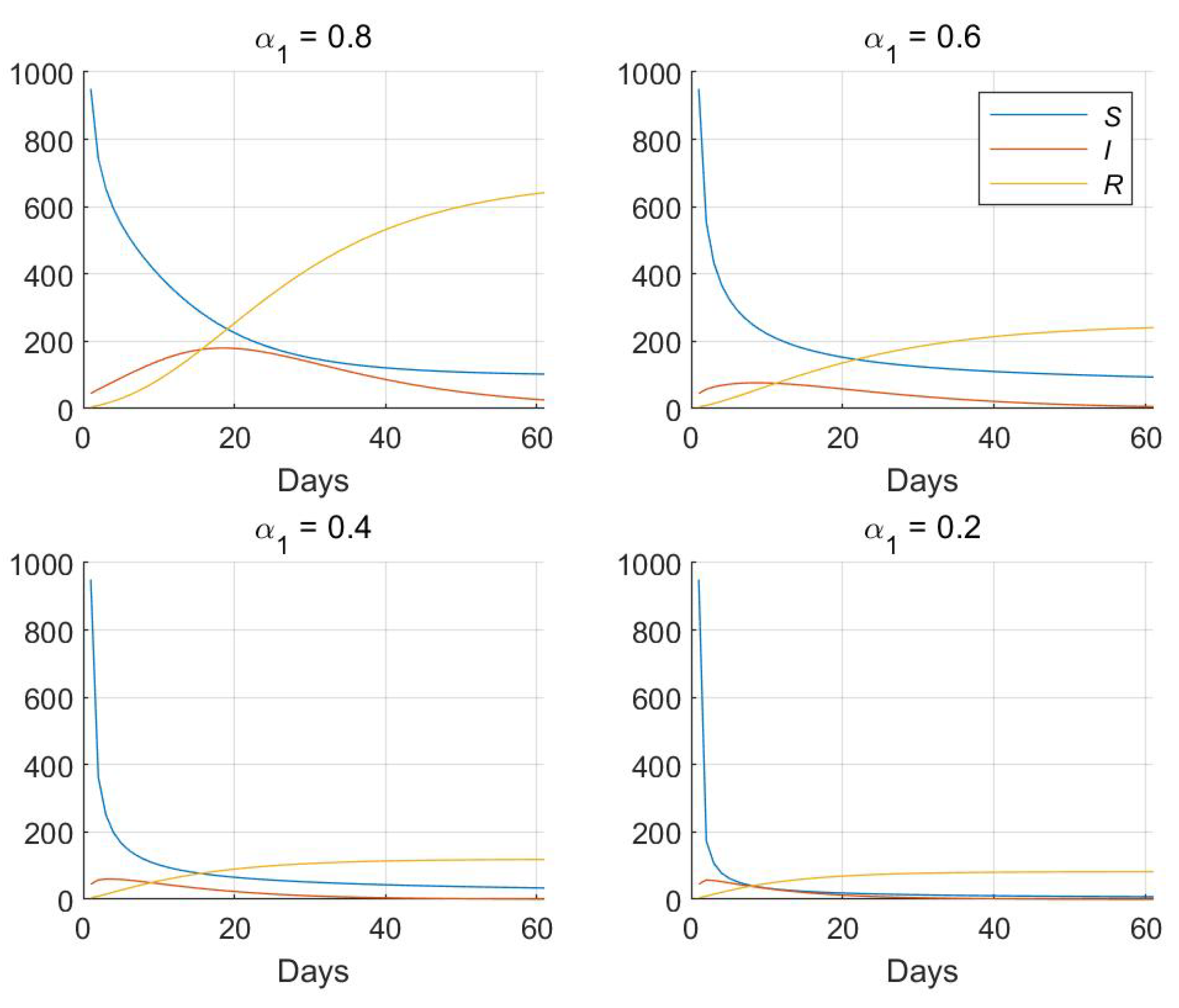
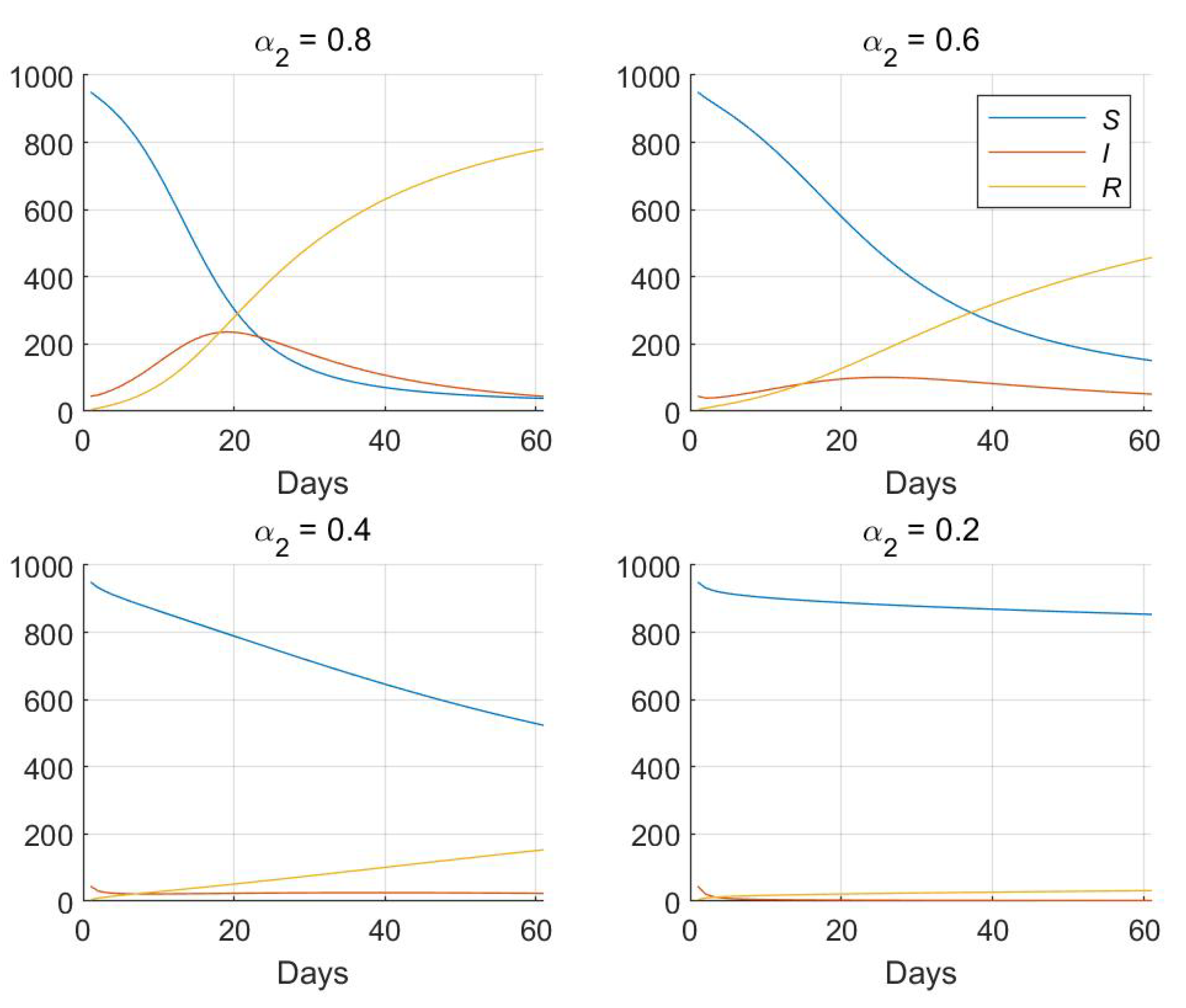
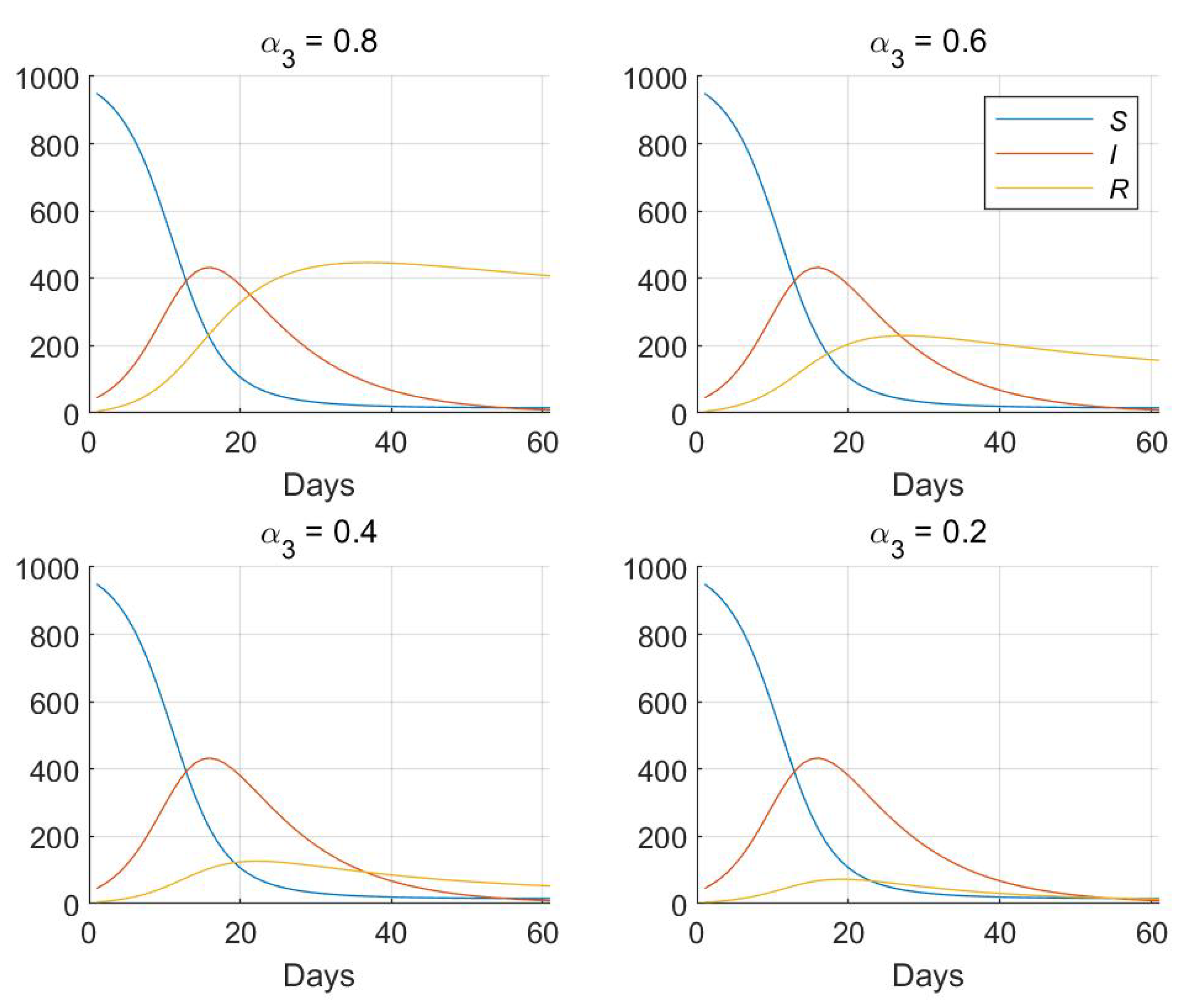
Consider three sets of simulations with following parameters: , and various . In each set, only one changes while two remain are equal to 1. That way, we can see how the particular fractional order , affects the model. Figure 1, Figure 2 and Figure 3 present the simulation results.
As we can see in Figure 1, Figure 2 and Figure 3, fractional orders and affect the whole model, while only affects the removed compartment. It can be expected if we look at the model’s Equation (9). With more parameters, the presented model is more complicated but is also more versatile. The results presented above show that fractional-order SIR can be more adjustable in the modeling of real-life processes.
4.2. Transmission Modeling for Italy and Spain
In this section, we implement the fractional-order SIR model in order to predict COVID-19 transmission for Italy and Spain.
In order to model the spread of COVID-19, we have model parameters, as follows . Accounting that the order does not affect model output I, for simplicity, we assume that . Parameter N is arbitrary given for each country. Therefore, using square lost function, we have to estimate four parameters , where and denotes modeled and actual number of infected individuals, respectively. In this paper, optimal model parameters are obtained the use of the Monte Carlo method based on the genetic algorithm.
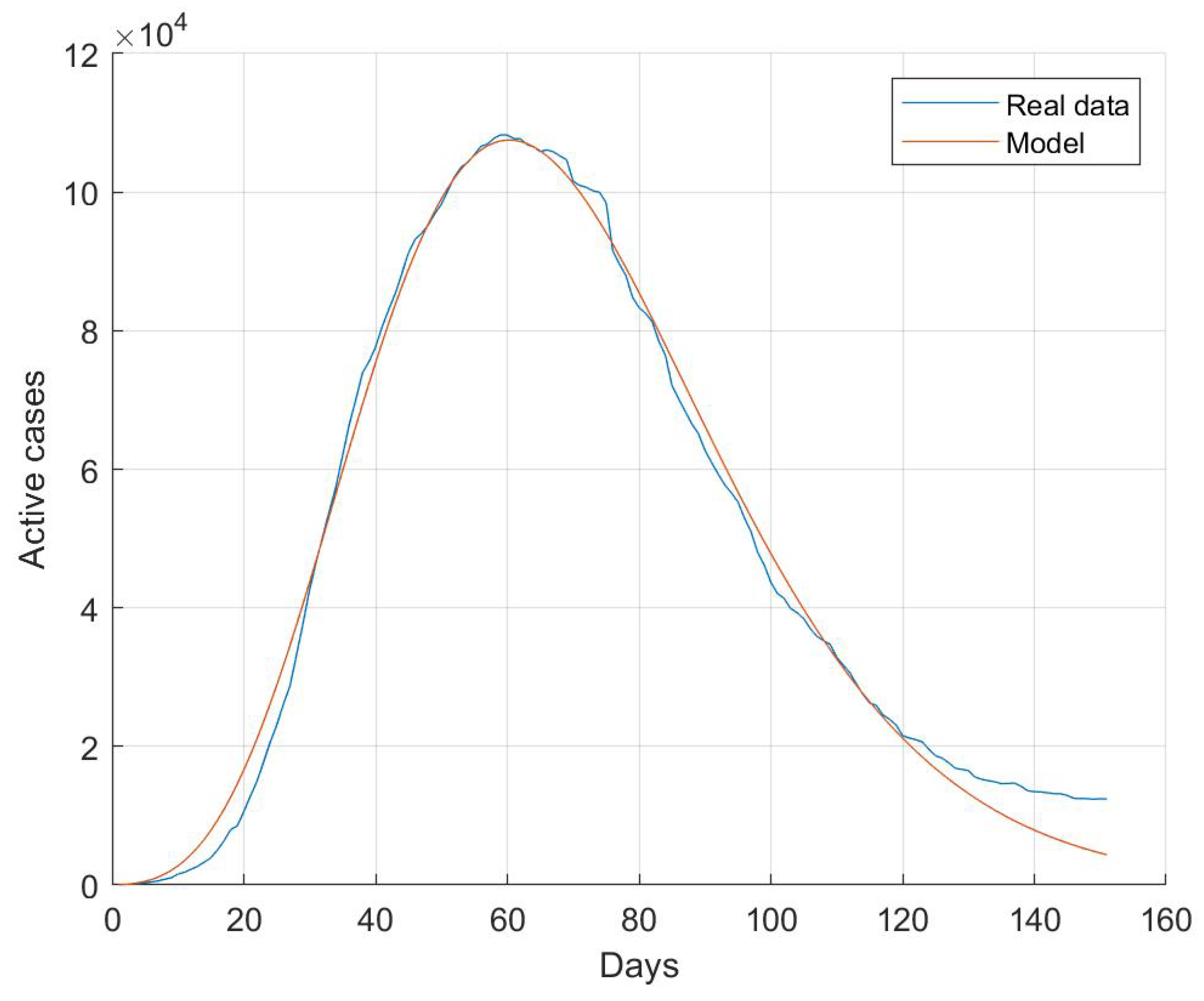
The starting point of simulation regarding the Italy epidemic is 21 February, when there were 19 active cases and 0 removed, so , , 60,461,828 and = 60,461,726. Using the above-presented optimization method for , we obtain parameters, as follows and . Figure 4 presents the time plots of modeled and actual disease transmission.
As we can see in Figure 4, the fractional-order SIR model is effective in modeling the COVID-19 transmission in Italy. The Root Mean Square Error, defined as with n denoting prediction range, and being the actual and modeled active cases, respectively, is as . Note that, for the first 30 days, the modeled transmission is higher than the actual one. This can be a result of relatively low daily tests when compared to the rest of the period. In contrast, for , the actual transmission is significantly higher than the modeled one. It may be the result of gradually easing the restrictions (from May 16, ).
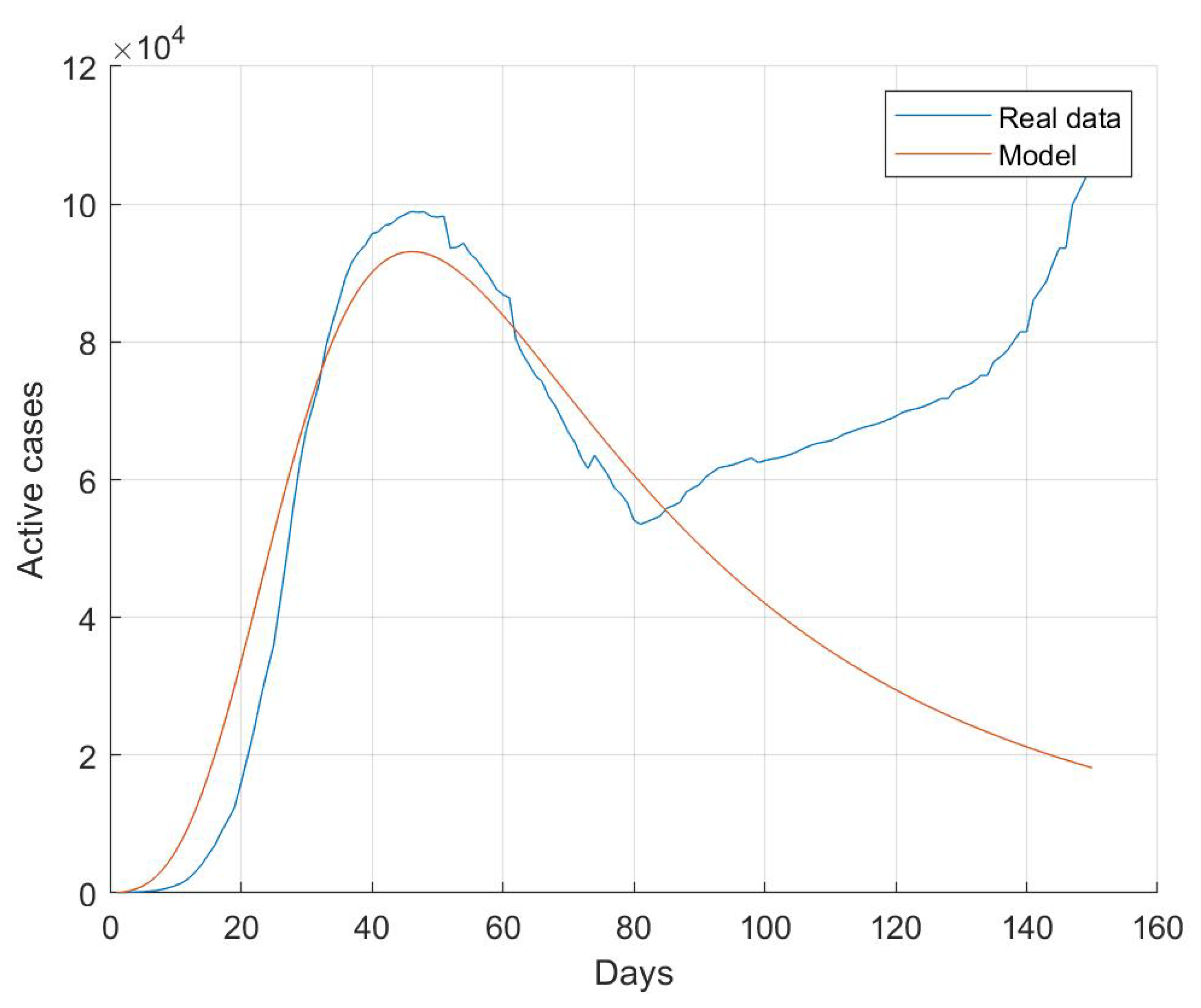
The starting point of simulation regarding the Spain epidemic is 27 February, when there were 31 active cases and 0 removed, so , , 46,757,240 and = 46,757,209. Using the optimization method for , we obtain parameters, as follows and . Figure 5 presents time plots of modeled and actual disease transmission.
The fractional-order SIR model is quite effective in modeling the COVID-19 transmission in Spain, as we can see in Figure 5. However, for , the actual transmission is significantly higher than the modeled one. Again, it may result from easing the restrictions (from 2 May, ). Furthermore, a resurgence is occurring in Spain, and the model is not capable of modeling this process. It is confirmed by RMSE, which, for , is equal to , but for is as . In this case, using time-varying model parameters may improve the fractional-order SIR model performances. However, using more complex models may be necessary in this case.
5. Conclusions
In this paper, the fractional-order generalization of the SIR epidemic model in order to predict the spread of the COVID-19 disease is presented. The model implementation is based on the Grünwald-Letnikov derivative and discretization while using the nabla fractional-order difference. We study the impact of fractional orders of the model derivatives on the dynamic properties of the proposed model. In modeling the COVID-19 transmission, the model’s parameters are estimated while using the genetic algorithm. The model prediction results for the spread of COVID-19 in Italy confirm the usefulness of the introduced methodology. However, modeling the results for Spain show that the model has some limitations. In the case of the second wave of the epidemic, the model’s prediction does not represent the real data. In this case, using time-varying parameters of the fractional-order SIR model or more complex pandemic models is necessary. Nevertheless, the study shows that the presented model is effective and it could be useful in future pandemics studies.
Author Contributions
Conceptualization, K.K. and R.S.; methodology, R.S.; software, K.K.; validation, K.K.; formal analysis, R.S.; investigation, K.K. and R.S.; resources, K.K.; data curation, K.K.; writing—original draft preparation, K.K. and R.S.; writing—review and editing, K.K., R.S. and G.B.; visualization, K.K. All authors have read and agreed to the published version of the manuscript.
Funding
This research received no external funding.
Conflicts of Interest
The authors declare no conflict of interest.
References
- Alamo, T.; Reina, D.; Mammarella, M.; Abella, A. COVID-19: Open-data resources for monitoring, modeling, and forecasting the epidemic. Electronics 2020, 9, 827. [Google Scholar] [CrossRef]
- Fanelli, D.; Piazza, F. Analysis and forecast of COVID-19 spreading in China, Italy and France. Chaos Solitons Fractals 2020, 134, 109761. [Google Scholar] [CrossRef] [PubMed]
- Maleki, M.; Mahmoudi, M.R.; Heydari, M.H.; Pho, K.H. Modeling and forecasting the spread and death rate of coronavirus (COVID-19) in the world using time series models. Chaos Solitons Fractals 2020, 140, 110151. [Google Scholar] [CrossRef] [PubMed]
- Shulgin, B.; Stone, L.; Agur, Z. Pulse vaccination strategy in the SIR epidemic model. Bull. Math. Biol. 1998, 60, 1123–1148. [Google Scholar] [CrossRef]
- Zaman, G.; Kang, Y.H.; Jung, I.H. Stability analysis and optimal vaccination of an SIR epidemic model. Biosystems 2008, 93, 240–249. [Google Scholar] [CrossRef]
- Cooper, I.; Mondal, A.; Antonopoulos, C.G. A SIR model assumption for the spread of COVID-19 in different communities. Chaos Solitons Fractals 2020, 139, 110057. [Google Scholar] [CrossRef]
- Kermack, W.; McKendrick, A. A contribution to the mathematical theory of epidemics. Proc. R. Soc. Lond. Ser. A Contain. Pap. Math. Phys. Character 1927, 115, 700–721. [Google Scholar] [CrossRef] [Green Version]
- Allen, L.J. Some discrete-time SI, SIR, and SIS epidemic models. Math. Biosci. 1994, 124, 83–105. [Google Scholar] [CrossRef]
- Kucharski, A.J.; Russell, T.W.; Diamond, C.; Liu, Y.; Edmunds, J.; Funk, S.; Eggo, R.M.; Sun, F.; Jit, M.; Munday, J.D.; et al. Early dynamics of transmission and control of COVID-19: A mathematical modelling study. Lancet Infect. Dis. 2020, 20, 553–558. [Google Scholar] [CrossRef] [Green Version]
- Sarkar, K.; Khajanchi, S.; Nieto, J.J. Modeling and forecasting the COVID-19 pandemic in India. Chaos Solitons Fractals 2020, 139, 110049. [Google Scholar] [CrossRef]
- Giordano, G.; Blanchini, F.; Bruno, R.; Colaneri, P.; Filippo, A.D.; Matteo, A.D.; Colaneri, M. Modelling the COVID-19 epidemic and implementation of population-wide interventions in Italy. Nat. Med. 2020, 26, 855–860. [Google Scholar] [CrossRef] [PubMed]
- Ndaïrou, F.; Area, I.; Nieto, J.J.; Torres, D.F.M. Mathematical modeling of COVID-19 transmission dynamics with a case study of Wuhan. Chaos Solitons Fractals 2020, 135, 109846. [Google Scholar] [CrossRef] [PubMed]
- Atangana, A.; Gómez-Aguilar, J. Fractional derivatives with no-index law property: Application to chaos and statistics. Chaos Solitons Fractals 2018, 114, 516–535. [Google Scholar] [CrossRef]
- Ghanbari, B.; Atangana, A. A new application of fractional Atangana–Baleanu derivatives: Designing ABC-fractional masks in image processing. Phys. A Stat. Mech. Appl. 2020, 542, 123516. [Google Scholar] [CrossRef]
- Morales-Delgado, V.F.; Gómez-Aguilar, J.F.; Saad, K.; Jiménez, R.F.E. Application of the Caputo-Fabrizio and Atangana-Baleanu fractional derivatives to mathematical model of cancer chemotherapy effect. Math. Methods Appl. Sci. 2019, 42, 1167–1193. [Google Scholar] [CrossRef]
- Khan, M.A.; Atangana, A. Modeling the dynamics of novel coronavirus (2019-nCov) with fractional derivative. Alex. Eng. J. 2020, 59, 2379–2389. [Google Scholar] [CrossRef]
- Srivastava, H.M.; Günerhan, H. Analytical and approximate solutions of fractional-order susceptible-infected- recovered epidemic model of childhood disease. Math. Methods Appl. Sci. 2019, 42, 935–941. [Google Scholar] [CrossRef]
- Abdo, M.S.; Shah, K.; Wahash, H.A.; Panchal, S.K. On a comprehensive model of the novel coronavirus (COVID-19) under Mittag-Leffler derivative. Chaos Solitons Fractals 2020, 135, 109867. [Google Scholar] [CrossRef]
- Grünwald, A.K. Ueber “begrenzte” Derivationen und deren Anwendung. Z. Math. Phys. 1867, 12, 441–480. [Google Scholar]
- Dzieliński, A.; Sierociuk, D.; Sarwas, G. Some applications of fractional order calculus. Bull. Pol. Acad. Sci. Tech. Sci. 2010, 58. [Google Scholar] [CrossRef] [Green Version]
- Kopka, R. Changes in Derivative Orders for Fractional Models of Supercapacitors as a Function of Operating Temperature. IEEE Access 2019, 7, 47674–47681. [Google Scholar] [CrossRef]
- Magin, R.L.; Ingo, C. Entropy and Information in a Fractional Order Model of Anomalous Diffusion. IFAC Proc. Vol. 2012, 45, 428–433. [Google Scholar] [CrossRef]
- COVID-19 Coronavirus Pandemic. Available online: https://www.worldometers.info/coronavirus/ (accessed on 5 August 2020).
- WHO Coronavirus Disease (COVID-19) Dashboard. Available online: https://covid19.who.int/ (accessed on 14 August 2020).
Figure 1.
Simulation results for various and .

Figure 2.
Simulation results for various and .

Figure 3.
Simulation results for various and .

Figure 4.
Modeled vs. actual disease transmission in Italy.

Figure 5.
Modeled vs. actual disease transmission in Spain.

Publisher’s Note: MDPI stays neutral with regard to jurisdictional claims in published maps and institutional affiliations. |
© 2020 by the authors. Licensee MDPI, Basel, Switzerland. This article is an open access article distributed under the terms and conditions of the Creative Commons Attribution (CC BY) license (http://creativecommons.org/licenses/by/4.0/).
Share and Cite
MDPI and ACS Style
Kozioł, K.; Stanisławski, R.; Bialic, G. Fractional-Order SIR Epidemic Model for Transmission Prediction of COVID-19 Disease. Appl. Sci. 2020, 10, 8316. https://doi.org/10.3390/app10238316
AMA Style
Kozioł K, Stanisławski R, Bialic G. Fractional-Order SIR Epidemic Model for Transmission Prediction of COVID-19 Disease. Applied Sciences. 2020; 10(23):8316. https://doi.org/10.3390/app10238316
Chicago/Turabian StyleKozioł, Kamil, Rafał Stanisławski, and Grzegorz Bialic. 2020. "Fractional-Order SIR Epidemic Model for Transmission Prediction of COVID-19 Disease" Applied Sciences 10, no. 23: 8316. https://doi.org/10.3390/app10238316
Note that from the first issue of 2016, this journal uses article numbers instead of page numbers. See further details here.