The Ability of Selected European Countries to Face the Impending Economic Crisis Caused by COVID-19 in the Context of the Global Economic Crisis of 2008

Abstract

This paper is devoted to the ability of selected European countries to face the potential economic crisis caused by COVID-19. Just as other pandemics in the past (e.g., SARS, Spanish influenza, etc.) have had negative economic effects on countries, the current COVID-19 pandemic is causing the beginning of another economic crisis where countries need to take measures to mitigate the economic effects. In our analysis, we focus on the impact of selected indicators on the GDP of European countries using a linear panel regression to identify significant indicators to set appropriate policies to eliminate potential negative consequences on economic growth due to the current recession. The European countries are divided into four groups according to the measures they took in the fiscal consolidation of the last economic crisis of 2008. In the analysis, we observed how the economic crisis influences GDP, country indebtedness, deficit, tax collection, interest rates, and the consumer confidence index. Our findings include that corporate income tax recorded the biggest decline among other tax collections. The interest rate grew in the group of countries most at risk from the economic crisis, while the interest rate fell in the group of countries that seemed to be safe for investors. The consumer confidence index can be considered interesting, as it fell sharply in the group of countries affected only minimally by the crisis (Switzerland, Finland).

1. Introduction

The current situation caused by COVID-19 is resulting in economic depression in practically every developed economy of the world. As with other diseases of the past, e.g., SARS, Spanish influenza, etc., with each pandemic, countries had to deal with an economic recession (Garret 2007; Lee and McKibbin 2004; Qiu et al. 2018). The COVID-19 pandemic has affected the global economy in many ways, such as by affecting global demand, supply chains, labor supply, foreign trade, and other areas. According to the predictions made by Comisión Europea (2020a), it is likely that the EU has entered the deepest economic recession in its history. Economic activity in Europe dropped very fast in March 2020. Governments had to take precautionary public health measures, which completely stopped economic activity. It is assumed that the recession of the global economy will be sharper than during the global economic crisis. Data for the first quarter of 2020 confirmed significant consequences on the European economy of the COVID-19 pandemic (Comisión Europea 2020b). The real GDP growth in Q1 2020 was about −3% and for the year 2020 is forecasted to be −8.3% in the EU. It is expected that the European economy will bounce back at the end of 2020 and in 2021 but persistent differences among countries are assumed.

At present, the analysis of the previous global economic crisis in 2008 can still be considered highly useful, as the COVID-19 pandemic is having a negative impact on every advanced economy. Each crisis has specific causes and process but usually affects similar indicators, e.g., GDP, unemployment rate, public debt. According to Standard & Poor’s (2020), the European Manufacturing Purchasing Managers’ Index fell under 35 in April 2020, which is the same level as in 2009. The highest deviation from the normal level of economic activity was in April 2020. It was almost 25% lower than the normal level. The main contributions to this fall were wholesale and retail trade, manufacturing, and transportation. Growth of economic activity has occurred in the health sector during the COVID-19 pandemic (Moody’s Analytics 2020). Signs of the beginning of the recession and economic crisis can already be seen. For this reason, individual economies will introduce fiscal consolidation to mitigate the impact of the economic crisis. Also on the basis of this, it will be possible to observe individual economies to determine whether they will introduce similar measures in the area of fiscal consolidation to those used in the 2008 crisis. Currently, there are very few publications dealing with fiscal consolidation and the economic crisis caused by COVID-19. O’Connor et al. (2020) recently published a study examining how the U.S. economy and its health care system are affected by the COVID-19 crisis. They conclude that the return to normalcy will be slow and could be different to what we are accustomed to. De Vito and Gómez (2020) have tested how the COVID-19 health crisis could affect the liquidity of listed firms across 26 countries by stress-testing three liquidity ratios for each firm with full and partial operating flexibility in two simulated distress scenarios. The results are that the firms’ current liabilities would increase, on average by eight times. Moreover, about 1/10th of all sample firms would become illiquid. Finally, De Vito and Gómez (2020) study two different fiscal policies, tax deferrals and bridge loans, that governments could implement to mitigate the liquidity risk. They conclude that bridge loans are more cost-effective to prevent a massive cash crunch.

The last major economic recession in the EU was the economic crisis of 2008. During this crisis, individual EU countries proceeded to mitigate the effects of the crisis through fiscal consolidation. It is therefore highly assumed that countries will proceed with fiscal consolidation now. For this reason, our research is based on the fiscal consolidations of selected EU countries from 2008, where we are able to observe the possible current development of selected EU countries in mitigating the economic impacts caused by COVID-19. The aim of our research is to study how countries dealt with the 2008 global economic crisis and how they are able to face the new recession. In our paper, we do not compare the global economic crisis and current recession caused by the COVID-19. However, given the relatively short period between these recessions, we can expect the consequences of the 2008 crisis to affect how countries cope with the consequences of the current recession caused by the COVID-19 pandemic.

During a period of global financial and economic crisis, the role of government and its intervention in achieving economic objectives are applied through fiscal consolidation (OECD 2013). One of the significant factors that appear during a global financial crisis is the reduction of GDP and the rise of debt in all advanced economies. These factors had a negative impact on growth rates in fiscal consolidation. Fatás and Summers (2018) attempted to reduce debt through fiscal policy multipliers that led to a higher debt to GDP ratio through their long-term negative impact on output.

Attinasi and Metelli (2017) studied the effects of fiscal consolidation on the debt-to-GDP ratio of several countries in the Euro area during a period from 2000 to 2012. The study was conducted by using a quarterly panel vector autoregressive model (Panel VAR). This measure increases if government revenues affect the initial increase in the debt ratio and the debt ratio reverts to its pre-shock level, resulting in self-defeating consolidation. Another panel of several countries in the Euro area was set up for the period 1990–2012. This panel was used to analyze fiscal consolidation through the effects of the functional components and sub-components of government expenditures. The result claims that fiscal consolidation is harmful to social expenditures, mainly those related to citizens’ safety, as seen in the Portugal, Ireland, Italy, Greece, and Spain (PIIGS) countries (Castro 2017). In the context of the conditions of the euro area, other research was carried out by Anderson et al. (2014). The aim was to examine the scope for structural reforms in the euro area to offset the negative impact of fiscal consolidation that was required to put public debt back on a sustainable path. The researchers used IMF’s Global Integrated Monetary and Fiscal model, abbreviated as GIMF. The result suggested that it would take several years before structural reforms could return the level of output back to its pre-consolidation path. When talking about the condition of fiscal consolidation in the euro area, Antelo and Peón (2014) focused their research on fiscal imbalances and replacement of public debt among the peripheral countries of the euro area, known as the Greece, Italy, Portugal, Spain, and Ireland (GIPSI) or PIIGS countries. Their goal was to conduct a debate on fiscal austerity vs. growth in macroeconomic performance between the researchers and policymakers. The empirical analysis performed showed that the sustainability of public debt for GIPSI countries in different scenarios of growth, inflation, fiscal, and monetary policies would be sustainable if the GIPSI countries achieve both fiscal consolidation, and economic growth.

From the other point of view, the cost of credit increases fiscal consolidation when assisted by tax hikes and spending cuts. The higher tax hikes, the higher cost of credits appears in a particular sector, unlike the spending cuts that are directed to a certain sector (Ağca and Igan 2019). When talking about fiscal consolidation in the context of spending cuts vs. tax hikes, Erceg and Lindé (2013) have done other research. Their research used a DSGE model to examine the effects of tax-based vs. expenditure-based fiscal consolidation in a currency union. The results were summed up into three key findings, including that tax-based consolidation tends to have smaller adverse effects on output than expenditure-based consolidation in the near-term. Secondly, a large expenditure-based consolidation may be counterproductive in the near-term at certain points; lastly, a mixed strategy of both mentioned consolidations means a temporary rise in taxes with gradual spending cuts may be desirable in minimizing the output costs of fiscal consolidation. Lemoine and Lindé (2016) continued in the research of expenditure-based fiscal consolidation under imperfect credibility. The research was focused on the credibility impact in monetary policy and a currency union under certain conditions. The result was that under an independent monetary policy approach, the impact of limited credibility is small and consolidation should reduce government debt at a low output cost. Secondly, the lack of monetary accommodation under a currency union implies that the output cost can be larger and in the short and medium-term can be limited under imperfect credibility.

Talking about the fiscal consolidation in a field of monetary policy and credibility, new research of the fiscal consolidation from the banks’ point of view was offered by Cimadomo et al. (2014). They investigate the effects of fiscal policy on bank balance sheets by using a very large data set of individual banks’ balance sheets. They found that the Tier-1 ratio tends to improve following episodes of fiscal consolidation. Continuing on the fiscal consolidation of monetary policy, Caselli researched fiscal consolidation under fixed exchange rates by using the Obstfeld and Rogoff model. If home authorities alone are responsible for pegging the exchange rate, a fiscal adjustment leads to a decrease in the real interest rate, stimulates private consumption, and limits the contraction in world output, compared with a situation in which a cooperative scheme is implemented (Caselli 2001).

Several OECD countries were analyzed under the condition of fiscal consolidation and the effects of a fiscal adjustment simulation. The conducted simulation supports the hypothesis that the effects of consolidation depend on their design. The difference between tax-based and expenditure-based adjustments appears to not be explained by accompanying policies, including monetary policy (Alesina et al. 2015). On the other hand, OECD countries were tested in order to analyze what drives the short-run costs of fiscal consolidation on output and employment. The results were found to vary with the state of the business cycle, monetary policy, public debt, the current account, and private credit. The main finding was that short-term output multipliers are below unity, even in states in which multipliers are expected to be larger (Banerjee and Zampoli 2019). Alesina et al. (2017) investigated the macroeconomic effects of fiscal consolidation based upon government spending cuts, transfers, and tax hikes in OECD countries. Government spending cuts and cuts in transfers are as harmful than tax hikes, despite the fact that non-distortionary transfers are not classified as spending. Static disturbances caused by persistent tax hikes cause larger shifts in aggregate supply under sticky prices.

Lastly, there are several pieces of research focused on analyzing the success and failures of fiscal consolidation. Heylen and Everaert (2000) examined five hypotheses on the composition of the consolidation program, its size and persistence, the gravity of the debt situation, the influence of the international macroeconomic environment, and the contribution of a preceding evaluation. The result was that fiscal consolidation depends on the composition of the consolidation program. Von Hagen and Strauch (2001) analyzed the effects of successful fiscal consolidation on the quality of fiscal adjustments and economic conditions such as government budget consolidations in OECD countries. The cyclical positions of the domestic and international economy affect the government’s choice of consolidation strategy, making them important determinants of the success of fiscal consolidation. Reicher estimated fiscal rules for a cross-section of countries in order to analyze OECD countries and determine which instrument is most successful for the stabilization of fiscal consolidation. A number of commonalities and differences emerged. Usually, countries adjust tax revenues in response to public debt and transfer payments. On the other hand, tax rates are not adjusted or government expenditures in response to output. These results support some recent developments in the theoretical literature, namely an increased emphasis on the effects of countercyclical transfer payments as an anti-cyclical fiscal policy instrument (Reicher 2014).

2. Materials and Methods

Our research is based on the (OECD 2011) analysis, which divided OECD member countries into four groups according to their consolidation plans after the financial crisis in 2009. The first group of countries is typical, meaning their fiscal consolidation was conducted after market pressures developed. Countries in the second group realized preventive fiscal consolidation. The third group consists of countries that needed fiscal consolidation, but they did not present it in 2011. The last group had low fiscal consolidation needs.

We focused on our research only on European countries. Due to data availability, we omitted countries with incomplete data. Therefore, our final dataset consists of the following countries. There are five countries in the first group: Hungary, Ireland, Spain, Portugal, and Greece. The second group consists of Germany, the Netherlands, Slovakia, and the United Kingdom. In the third group, there are Poland and France. The last group involves Switzerland, Finland, and Sweden. The analyzed period is from 2001 to 2017. The source of all data used in our analysis is the OECD database except for GDP, which comes from the Eurostat database (Supplementary Materials).

Due to the panel structure of our dataset, we applied the panel model analysis to study the impact of the tax revenues on GDP. Our model is defined by Equation (1), where GDP denotes gross domestic product in millions. EUR, CITR is corporate income tax revenue as a percentage of GDP, PITR is private income tax revenue as a percentage of GDP, PTR represents property tax revenue as a percentage of GDP, and GTR is goods and services tax revenue as a percentage of GDP. We also included four control variables: DEF—the balance of the state budget as a percentage of GDP, DEBT—public debt as a percentage of GDP, IR—annual interest rate of government bonds, and CCI—the consumer confidence index. Indexes i and t denote country and year, respectively. Parameters α and β represent regression coefficients and u is a random disturbance term of mean 0.

GDP_it = α_it + β_1it PITR_it + β_2it CITR_it + β_3it PTR_it + β_4it GTR_it + β_5it DEF_it + β_6it DEBT_it + β_8it IR_it + β_8it CCI_it + u_it,

(1)

We used two models for each group. The first model is the pooling model and the second is the fixed effects model. To decide which model is better, we applied the Poolability test (Croissant and Millo 2008). We do not use the random effects model because the third group consists of only two countries, which could lead to estimation inaccuracy. According to the theory, the structure of the dataset supposes the existence of fixed effects (Williams 2015). To decide between individual and time effects, we applied the Honda F test (Honda 1985). The OLS estimation requires several prerequisites to be met. The existence of the heteroscedasticity was tested by using the Pearson’s test (Plackett 1983). We used the Wooldridge test to identify the autocorrelation in the dataset (Wooldridge 2002). If the assumptions of the OLS estimation are violated, then a robust estimation would be applied (White 1980).

3. Results

Our analysis is divided into two parts. Firstly, we describe the development of selected economic indicators and in the second part, we develop linear panel models for each group of countries.

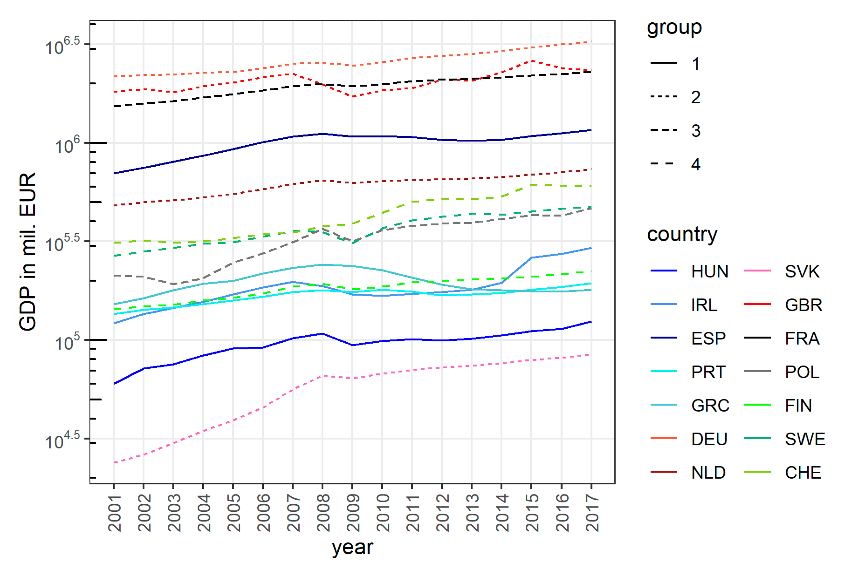
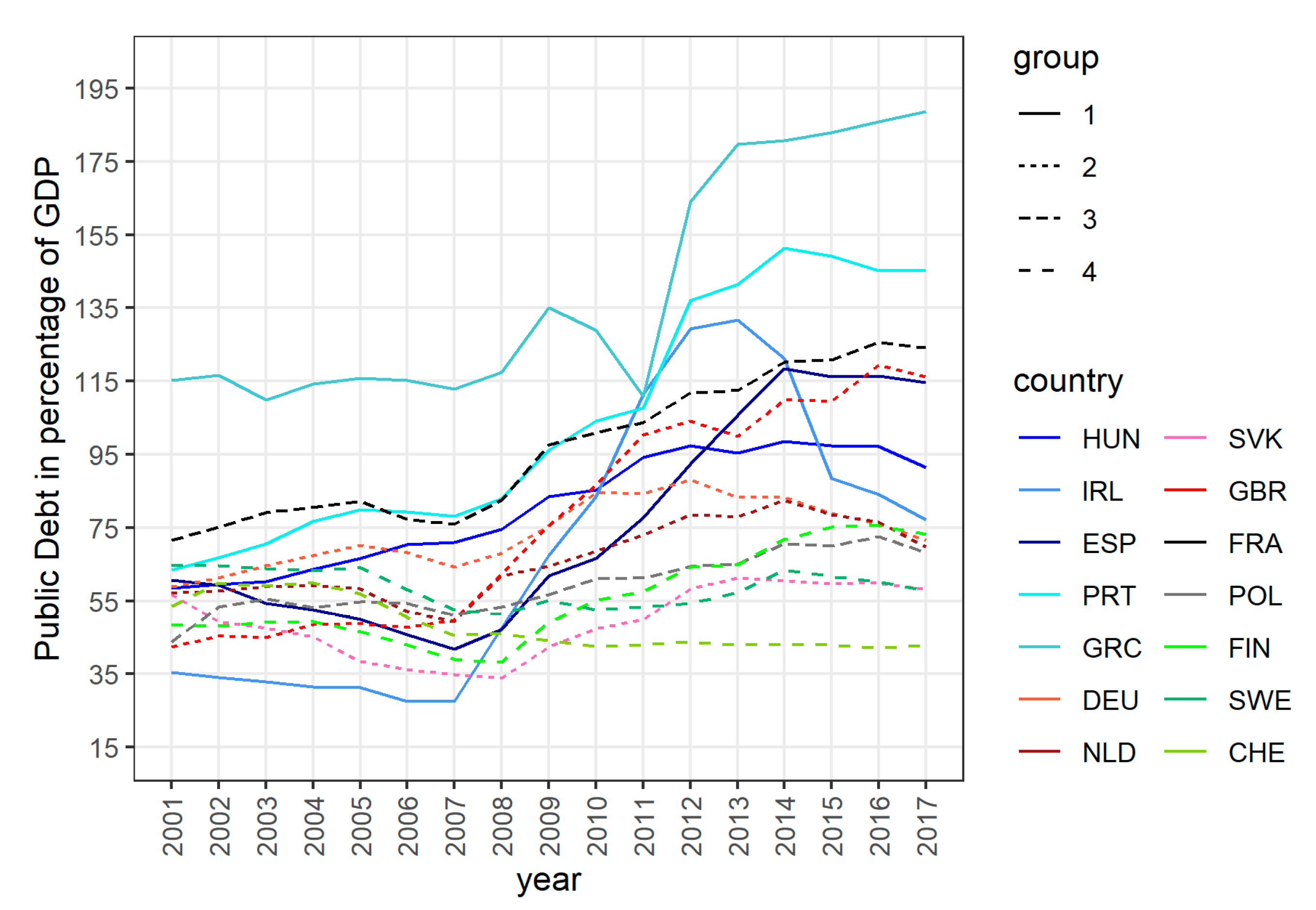
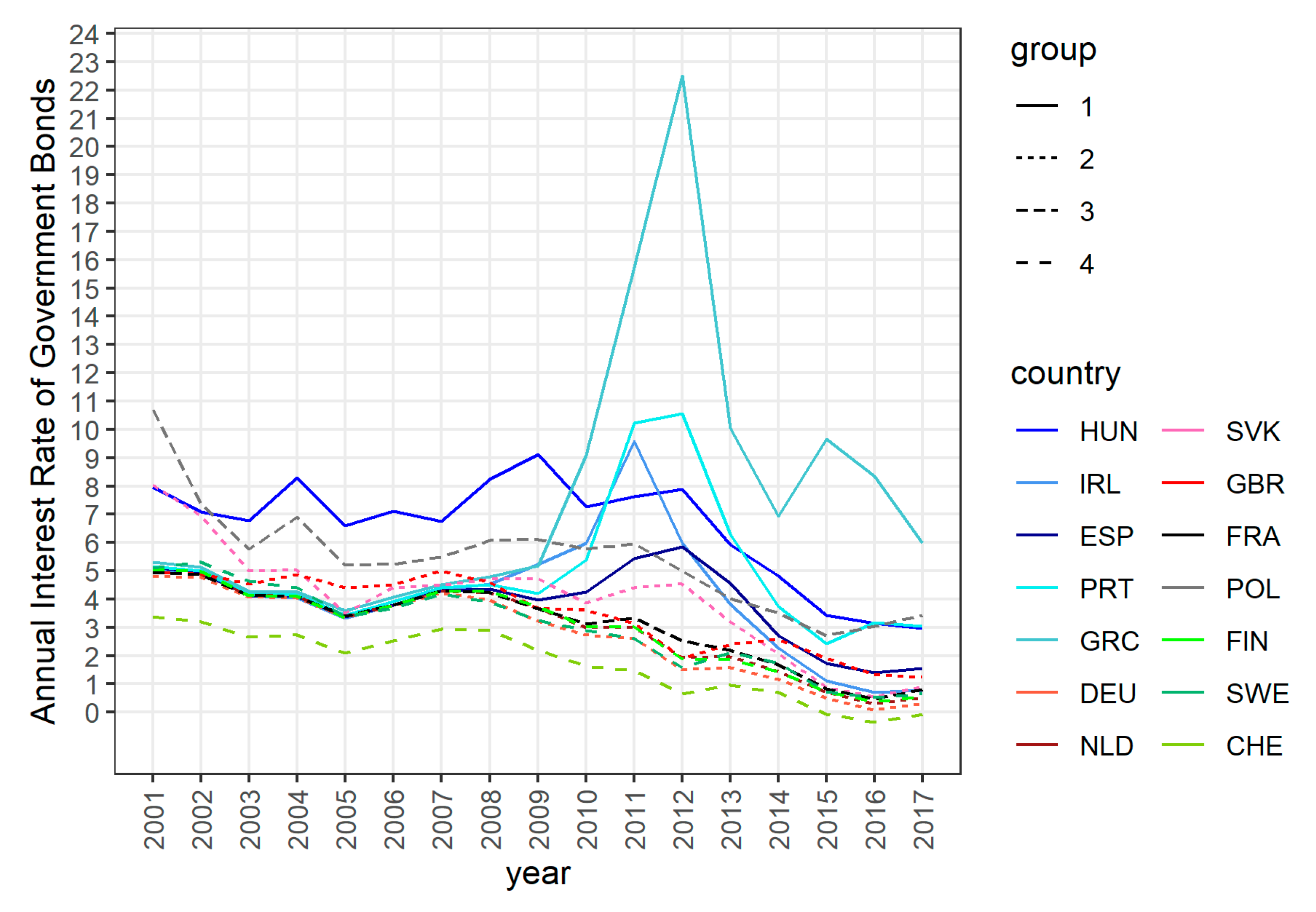
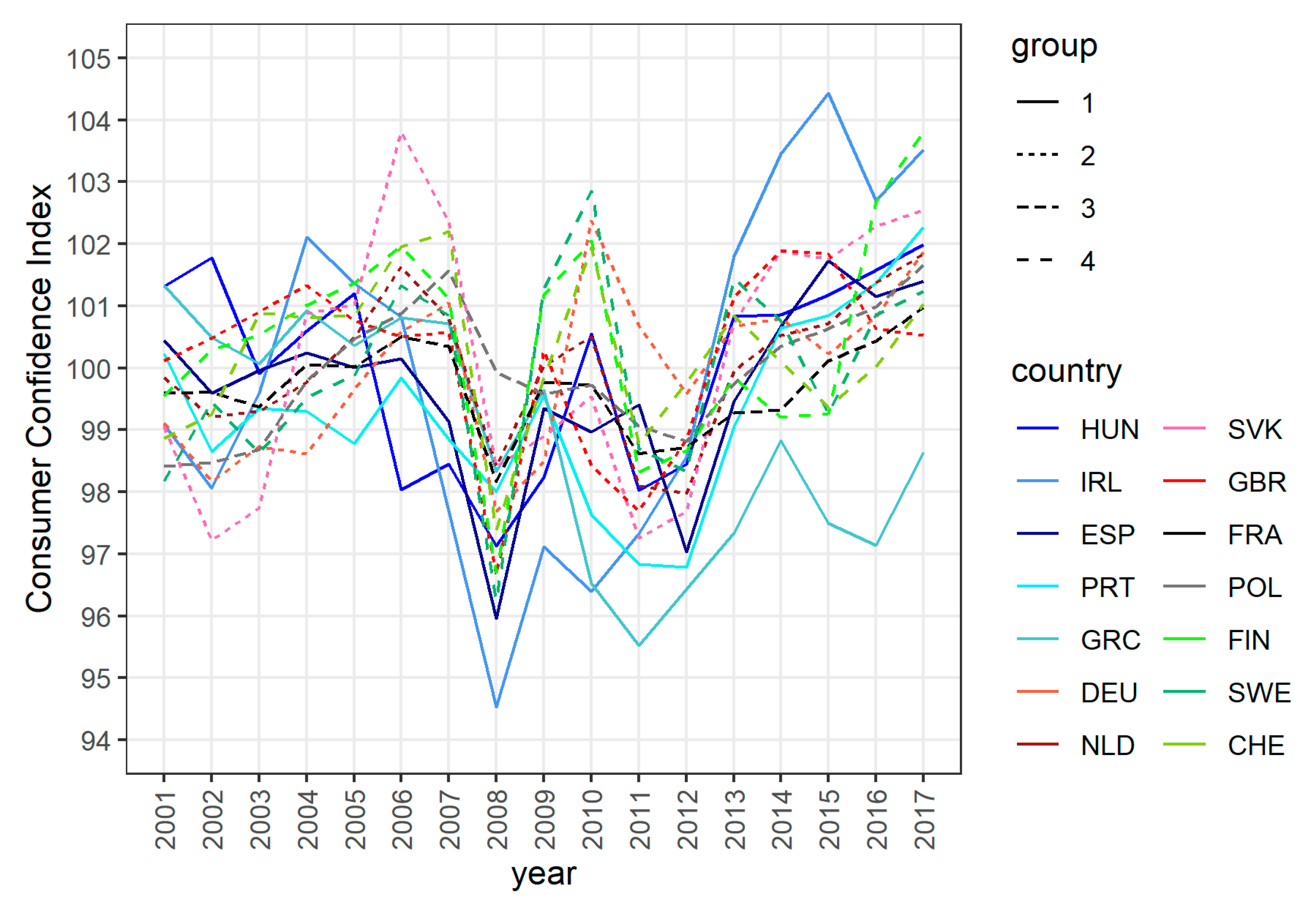
3.1. Economic Indicators Development

An economic crisis entails a decrease in economic performance. Commonly, economic performance is measured by GDP. In Figure 1, the development of the GDP in all analyzed countries is presented. The colors represent individual countries and line type denotes the group in which country belongs. The GDP of all countries has increased during the analyzed period. In all selected countries, the GDP decreased during the global economic crisis, but we can see different reactions among the countries. The first type of reaction is a significant drop in 2009, which was obvious in Hungary, Sweden, Poland, and the United Kingdom. In the case of the United Kingdom, the decrease started in 2008.

The other type of reaction is a moderate decrease with the bottom reached later than in 2009. This was the case for Greece, Portugal, and Spain. The last type was an only insignificant and slight decrease, e.g., in France, Switzerland, and Slovakia. It is important that there is no relationship between the reaction of the economy measured by the development of the GDP and policy applied by countries, which is categorized by their division into groups by the OECD.

To minimize the consequences of the economic crisis, governments increase public expenditures, which has a negative impact on public debt. Countries with low public debt have a larger space to eliminate crisis consequences. It is important to note this, especially in the time of the COVID-19 pandemic when governments need to spend a large amount of money. When we look at Figure 2, only Switzerland’s public debt did not increase in 2009. In all other countries, public debt increased after 2008 and in most of them, the public debt increased rapidly. In the context of the COVID-19 pandemic, it is essential to obtain a comparison of the public debt before the global economic crisis and now. In all analyzed countries, the public debt is higher now than it was before 2009 except for Switzerland and Sweden. This means that governments have not been able to cope with the previous global economic crisis, despite consolidation measures. Due to that fact, countries are currently in a worse position than in 2008 to realize expansive fiscal policy to eliminate crisis consequences and to start economic growth. According to Figure 2, the highest debt as a percentage of GDP was in 2017 in Greece, Portugal, France, the United Kingdom, and Spain. The threat for France, the United Kingdom, and Hungary is still growing public debt with a high probability of the next increase occurring due to the COVID-19 crisis.

The main component of the public debt is the deficit of the state budget, which increased in all countries in 2009. Only Switzerland’s state budget has been in surplus during the economic crisis in 2009. The largest deficit was in Ireland in 2010. This deficit was more than 31 percent of GDP, which is depicted in Figure 3. In the case of the state budget balance, there is an obvious positive trend indicating that the deficit has decreased and that differences among European countries have reduced over the studied period. It is necessary to mention that despite the strict regulations of the EU, most of the analyzed countries have still a deficit in their state budgets. This leads to public debt generation because governments obtain that missing money on the financial markets by selling government bonds.

The economic situation of a country affects investor confidence, which is expressed by the interest rate of that country’s government bonds. The development of the annual interest rates of government bonds during the analyzed period has a positive trend, which means that the government can borrow money more cheaply. The global economic crisis in 2009 did not disrupt that trend in most of the analyzed countries, which is depicted in Figure 4. There are only four countries with significant growth of their interest rates, specifically Greece, Portugal, Ireland, and Spain. On the other hand, there are countries with a low probability of bankruptcy, which were perceived as safe alternatives for investors and therefore their interest rates decreased in the 2008 economic crisis. This was the case for Switzerland, Finland, the United Kingdom, Sweden, and several others. Actual low interest rates provide a good position for governments to borrow money to cover their deficits. It is important to emphasize that financial markets are sensitive to economic stability and therefore interest rates in the case of countries with unstable economic development can grow markedly.

The economic situation also affects consumer behavior. Negative moods among consumers cause them to spend less, which can result in a larger recession. In Figure 5, we can see the development of consumer confidence index (CCI) trends. In countries with larger economic slumps, the CCI decreased more than in countries with better economic development. Sweden was not significantly affected by the global economic crisis but the CCI in Sweden dropped markedly. A similar situation occurred for Finland, Switzerland, and the United Kingdom. In 2017, the highest CCI was in Finland and the second-highest was in Ireland. It seems that consumers in these countries are very sensitive to the economic situation in their country. During the good economic phase, their mood is very positive, but their mood can change rapidly, which occurred in 2008. Especially in these countries, policymakers should use their measures to retain a positive consumer mood.

Taxation is the main source of income in a state’s budget. Countries differ in the tax systems used, but it is possible to generalize them. The first type of tax is private income tax. The share of that tax on GDP depends on the redistribution policy applied in a country. The largest share of this type of tax in the broader taxation base is in Sweden and Finland, which are typically countries with a high redistribution rate. On the other hand, the lowest share is in Slovakia and Poland. A significant decline in taxation caused by the 2008 global economic crisis was seen in Sweden and Spain, which is presented in Figure 6.

According to Figure 7, the share of the corporate income tax revenue on the GDP markedly lower than in the case of private income tax revenue. This is the result of efforts to increase competitiveness. Unlike citizens, companies can change their national residence to optimize their taxes. For corporate tax revenue, the consequences of an economic crisis are more visible. A huge slump occurred in Spain, France, and Hungary. After the 2008 economic crisis, the share of the tax base made up by corporate tax revenue increased in all the analyzed countries. The countries with a low share are Germany, Poland, and Hungary. In contrast, the highest share is in Slovakia, Netherlands, Switzerland, and Portugal.

The third group of taxes consists of property taxes. The share of these taxes varies from 0.5% in Slovakia up to more than 4% in France and the United Kingdom. During the global economic crisis, revenues from property taxes have markedly declined in Spain and Ireland, which can be seen in Figure 8. A significant increase after the economic crisis has occurred in Greece, which is associated with fiscal consolidation to meet European Union requirements. A similar development has been observed in Ireland and Spain. Analyzed countries vary significantly in case of the share of the property tax revenue on GDP.

The last group of taxes consists of indirect taxes, such as Value Added Tax and other consumption taxes. This group of taxes has the highest share of GDP in almost all analyzed countries. The highest share has been during the entire analyzed period in Hungary, followed by Finland and Portugal. The lowest share has been observed in Switzerland in all analyzed years. As is shown in Figure 9, a significant impact of the economic crisis on these indirect taxes has occurred in Spain and Portugal. Since all tax revenues in our analysis are expressed as the share of GDP, this does not mean that if there is no change in share of the tax revenue on the GDP then the economic crisis did not affect them, but rather that GDP and tax revenues change equally.

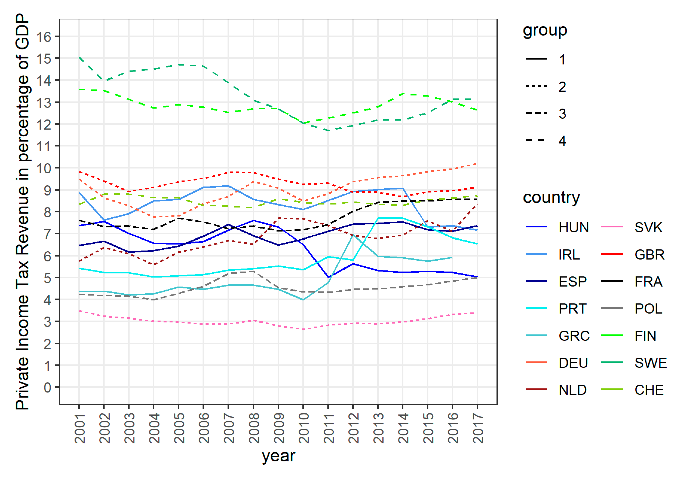
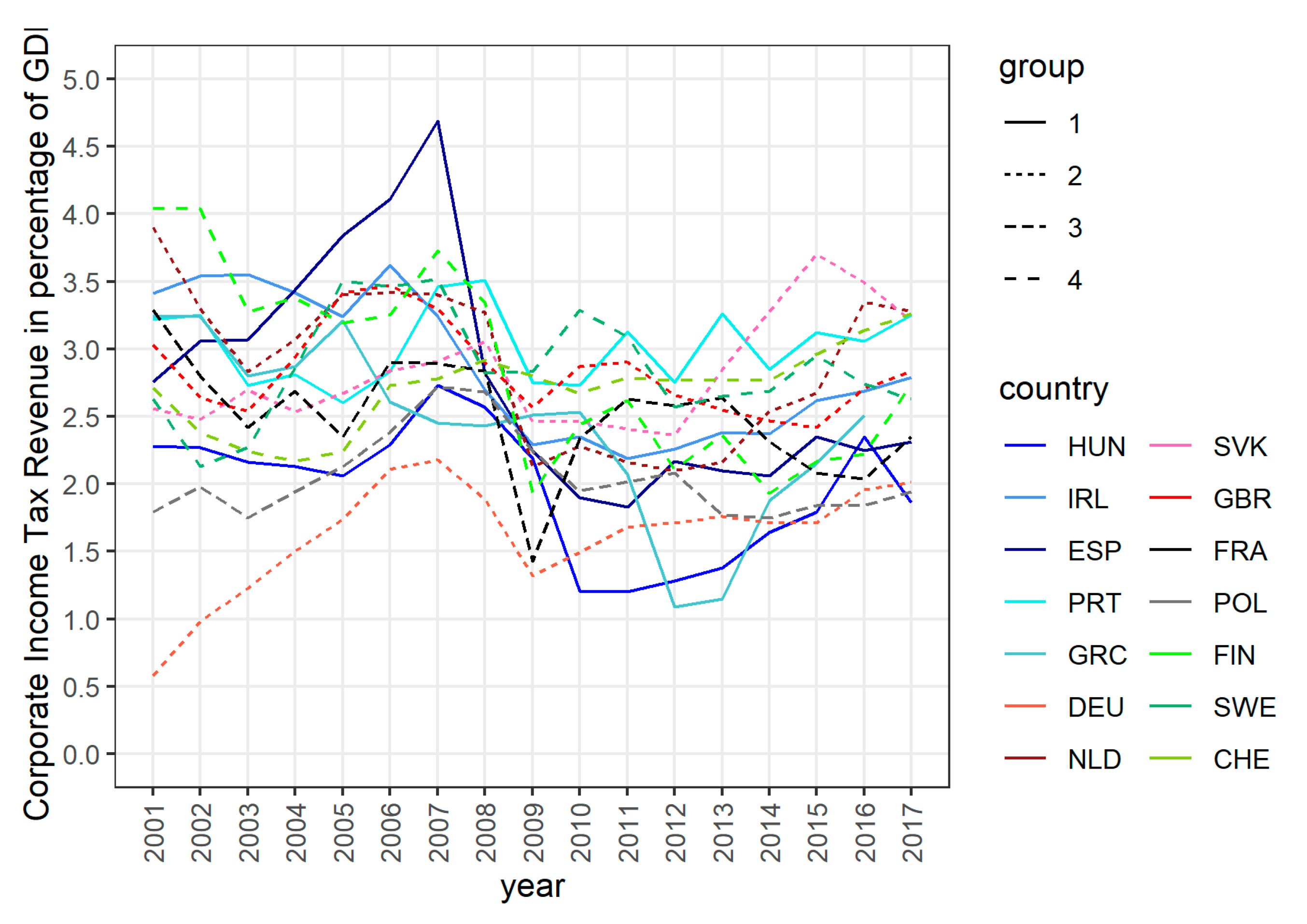
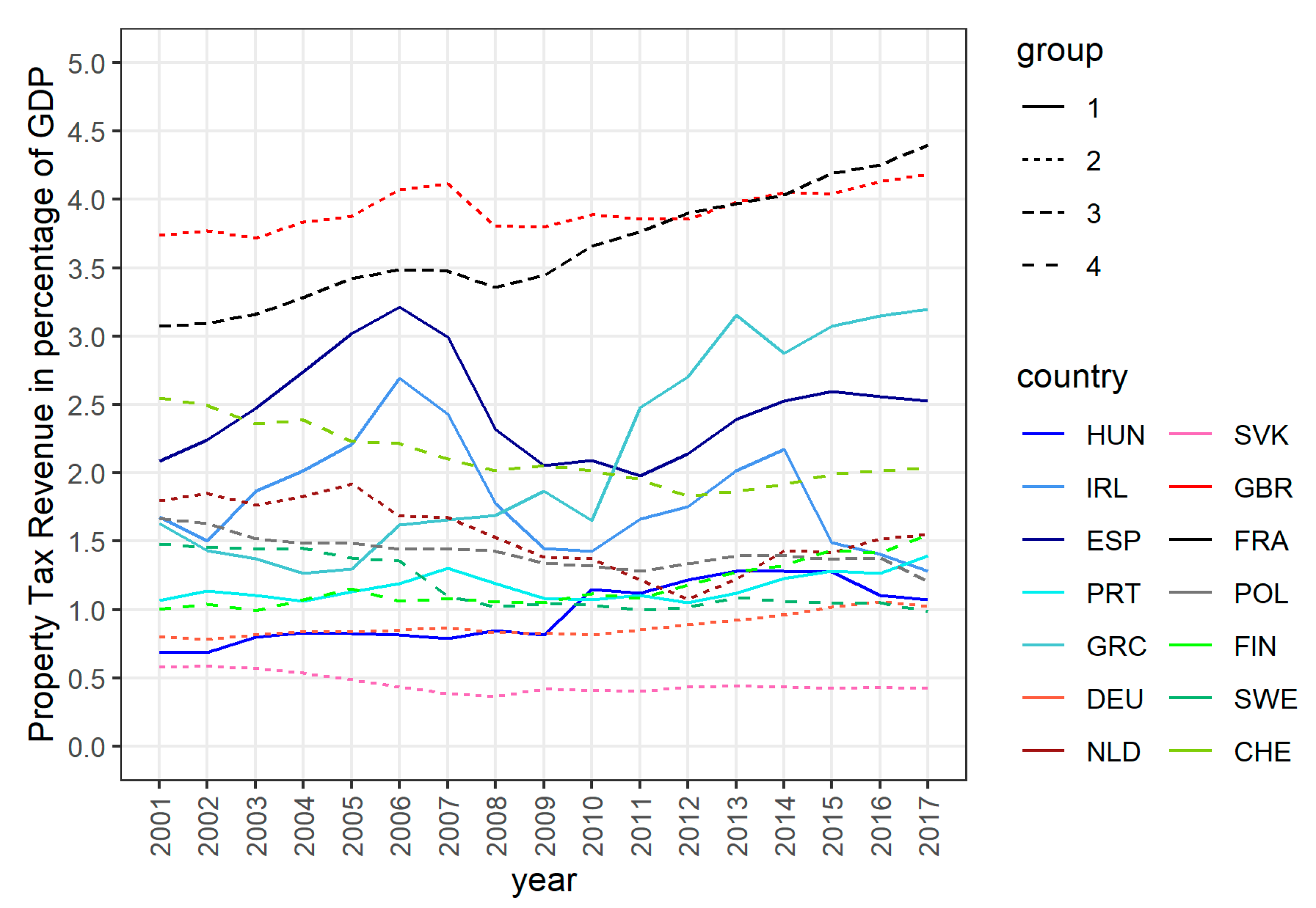
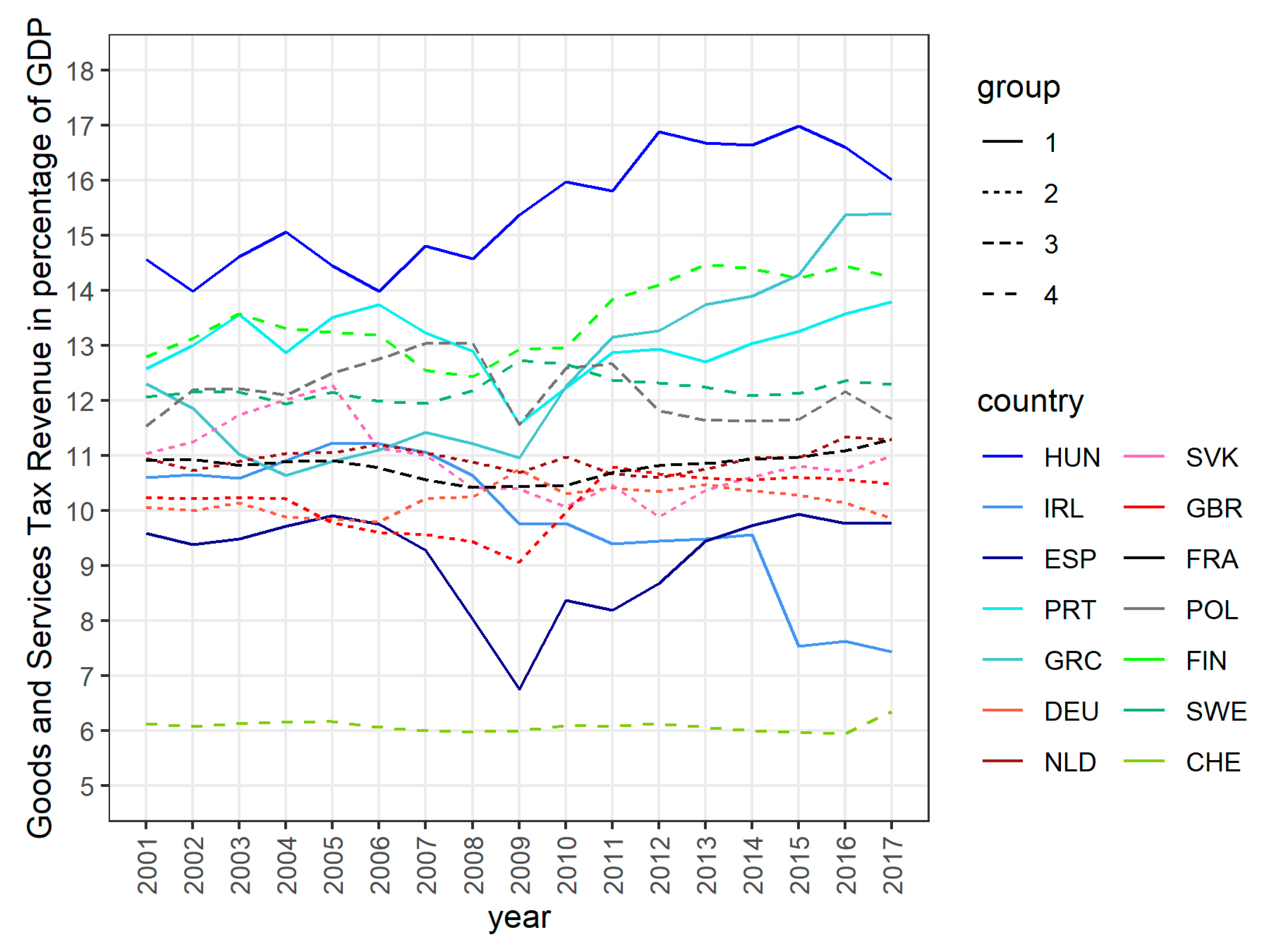
3.2. The Impact of Tax Revenues on the GDP

Changes in economic activity are often associated with tax collections. A decrease in economic activity in the form of lower consumption and investment leads to lower tax collections for the state budget. In the following analysis, we study relationships between tax collections of several types of taxes and GDP. To analyze the impact of tax revenues on the GDP, we developed four linear panel models. For each group described in the methodology, we built models separately.

3.2.1. Group 1

The first group consists of the following countries: Hungary, Ireland, Spain, Portugal, and Greece. According to the Poolability test, the appropriate model is the Fixed effects model (FM). There are only two statistically significant variables: CITR and GTR with significance levels of 10%. The increase of the CITR was by one million. EUR leads to a decrease in the GDP by 28 billion EUR. A similar situation is in the case of the GTR when an increase by one million causes the decrease of the GDP by 37 billion EUR. Other variables are not statistically significant in that model. Estimated coefficients are presented in

Table 1. Estimated models for the first group of countries.

	PM		FM
	Regression Coefficient	p-Value	Regression Coefficient	p-Value
PITR	−46,153.7	0.027	5775.6	0.700
CITR	−144,551	0.002	−28,025.5	0.020
PTR	227,780.3	<0.001	72,750.3	0.113
DEF	9738.6	0.19	94.7	0.959
DEBT	−1384.1	0.11	315.5	0.234
GTR	−70,369.5	<0.001	−37,311.2	0.007
IR	−26,952.9	0.025	−11,077.7	0.203
CCI	−25,030.1	0.187	−8995.2	0.119

Note: PM—Pooling model, FM—fixed effects model, PITR—private income tax revenue, CITR—corporate income tax revenue, PTR—property tax revenue, DEF—the balance of the state budget, DEBT—public debt, GTR—goods and services tax revenue, IR—annual interest rate of government bonds, CCI—consumer confidence index. Based on the Poolability test, the panel model is preferred (F = 11.401, p-value < 0.001). According to the F test, there are statistically significant individual effects (F = 19.465, p-value < 0.001) but statistically insignificant time effects (F = −2.653, p-value = 0.996). The Pearson test confirmed the existence of heteroscedasticity (χ² = 3, p-value = 0.003). The autocorrelation was not identified in the model by the Wooldridge test (χ² = 1.67, p-value = 0.096). Because of the heteroscedasticity, we applied a robust covariance estimation.

.

3.2.2. Group 2

There were the following countries in the second group: Germany, the Netherlands, Slovakia, and the United Kingdom. These countries took preventative measures to stabilize public finances due to the 2008 global financial crisis. For countries in the second group, the statistically significant variables are PITR, PTR, DEF, and GTR. We preferred Fixed effects model (FM) with the Poolability test. Based on the estimated coefficients shown in

Table 2. Estimated models for the second group of countries.

	PM		FM
	Regression Coefficient	p-Value	Regression Coefficient	p-Value
PITR	185,843.7	0.000	136,700.6	0.000
CITR	−516,424.0	0.000	−101,089.0	0.079
PTR	94,962.0	0.275	577,000.1	0.000
DEF	92,066.7	0.001	30,460.0	0.007
DEBT	11,980.6	0.006	4262.9	0.021
GTR	−458,229.0	<0.001	−74,839.1	0.084
IR	67,232.6	0.161	−29,486.8	0.149
CCI	87,290.1	0.019	10,309.4	0.458

Note: PM—Pooling model, FM—fixed effects model, PITR—private income tax revenue, CITR—corporate income tax revenue, PTR—property tax revenue, DEF—the balance of the state budget, DEBT—public debt, GTR—goods and services tax revenue, IR—annual interest rate of government bonds, CCI—consumer confidence index. The Poolability test favors the panel model (F = 4.010, p-value < 0.001). The F test confirmed the existence of individual effects (F = 8.836, p-value < 0.001) but rejected the existence of time effects (F = −1.578, p-value = 0.943). The Pearson test did not confirm the heteroscedasticity in the model (χ² = 1.070, p-value = 0.282), wwhile the autocorrelation was not identified in the model by the Wooldridge test (χ² = 1.26, p-value = 0.210).

, tax revenues from direct taxes (private income tax and property tax) have a positive impact on GDP. An increase in both forms of tax revenue leads to the growth of the GDP. In the case of the PITR, is the increase was by 136,700 and for PTR it was 577,000. The indirect tax GTR has an indirect impact on the GDP. An increase in the GTR by one unit causes the decline of the GDP by 74. The deficit of the state budget (DEF) is also statistically significant and has a positive effect on the GDP.

3.2.3. Group 3

There are only two countries in the third group: France and Poland. These countries did not realize fiscal consolidation although it was needed. Based on the Poolability test, the fixed effects model was more appropriate for these countries. Statistically significant variables on the level of significance of 10% were PITR, PTR, and DEF. All of them had a positive sign, which means that their increase causes an increase in the GDP. Estimated models are shown in

Table 3. Estimated models for the third group of countries.

	PM		FM
	Regression Coefficient	p-Value	Regression Coefficient	p-Value
PITR	185,843.7	0.000	136,700.6	0.000
CITR	−516,424.0	0.000	−101,089.0	0.079
PTR	94,962.0	0.275	577,000.1	0.000
DEF	92,066.7	0.001	30,460.0	0.007
DEBT	11,980.6	0.006	4262.9	0.021
GTR	−458,229.0	<0.001	−74,839.1	0.084
IR	67,232.6	0.161	−29,486.8	0.149
CCI	87,290.1	0.019	10,309.4	0.458

Note: PM—Pooling model, FM—fixed effects model, PITR—private income tax revenue, CITR—corporate income tax revenue, PTR—property tax revenue, DEF—the balance of the state budget, DEBT—public debt, GTR—goods and services tax revenue, IR—annual interest rate of government bonds, CCI—consumer confidence index. The Poolability test shows that the panel model is more appropriate than the pooling model (F = 27.178, p-value < 0.001). The F test rejected the existence of individual effects (F = −0.960, p-value = 0.832) and time effects (F = 0.480, p-value = 0.315). According to the Pearson test, the heteroscedasticity is not presented in the model (χ² = −0.980, p-value = 0.330), while the autocorrelation was not identified in the model by the Wooldridge test (χ² = −1.410, p-value = 0.160).

.

3.2.4. Group 4

Countries in the fourth group did not need fiscal consolidation. These countries are Switzerland, Finland, and Sweden. The Poolability test favors the fixed effects model (FM). On a significance level of 10%, a statistically significant impacts on the GDP were found for PITR, CITR, DEF, DEBT, IR, and CCI. PITR and CITR had a positive impact on the GDP and DEF, while DEBT, IR, and CCI affected the GDP negatively. Estimated coefficients are presented in

Table 4. Estimated models for the fourth group of countries.

	PM		FM
	Regression Coefficient	p-Value	Regression Coefficient	p-Value
PITR	51,884.6	<0.001	25,508.9	0.000
CITR	59,293.7	0.029	38,597.4	0.015
PTR	−263,748	<0.001	−15,579.8	0.697
DEF	−19,901.1	0.009	−13,677.1	0.002
DEBT	1239.6	0.46	−4984.3	0.000
GTR	−88,139.1	<0.001	−21,602.6	0.127
IR	−51,410.8	<0.001	−55,667.6	0.000
CCI	−5,074.2	0.223	−5816.6	0.017

Note: PM—Pooling model, FM—fixed effects model, PITR—private income tax revenue, CITR—corporate income tax revenue, PTR—property tax revenue, DEF—the balance of the state budget, DEBT—public debt, GTR—goods and services tax revenue, IR—annual interest rate of government bonds, CCI—consumer confidence index. The Poolability test shows that the panel model is more appropriate than the pooling model (F = 5.080, p-value < 0.001). The F test confirmed the existence of individual effects (F = 2.690, p-value = 0.004) and rejected the existence of time effects (F = −0.520, p-value = 0.698). According to the Pearson test, the heteroscedasticity is not presented in the model (χ² = 1.240, p-value = 0.215), while the autocorrelation was not identified in the model by the Wooldridge test (χ² = 1.250, p-value = 0.213).

.

4. Discussion

The actual pandemic situation has markedly decreased economic activity, which has led to an economic recession. Government measures to prevent the spread of the COVID-19 have caused a sharp fall in the European economy. GDP of the EU fell by 3.2% in the first quarter of 2020 compared with the last quarter of 2019 (Comisión Europea 2020b). Current forecasts indicate a significant economic slump in 2020 (Fernandes 2020). According to the European Commission (Comisión Europea 2020b), it is assumed that EU annual real GDP growth in 2020 will be −8.3%. Despite the different causes, this resembles the global economic crisis in 2008–2009. In 2009, the annual real GDP growth was −4.3% in the EU, followed by 2.2% growth in 2010 and 1.8% growth in 2011. It is assumed that the COVID-19 crisis should last for a shorter period, but this depends on the epidemiological situation, especially the development of drugs and vaccines. The actual forecast for 2021 is 6.1% growth of real GDP in the EU (Comisión Europea 2020b). The second and next waves of the COVID-19 pose a current threat to economies (Leung et al. 2020). Governments have been forced to take confinement measures to limit the spread of the COVID-19 but also need to warm up the economy. That requires their preparedness to release money into the economy, which depends on how they dealt with the previous global economic crisis. Negative consequences that they have not been able to deal with may pose a risk for eliminating the effects of COVID-19 pandemic.

Our analysis has shown the consequences of the global economic crisis in 2008 on European economies. Significant changes in studied indicators have been observed. The impact of the reduced economic activity due to the economic crisis is seen in the decrease of the GDP (Dimitras et al. 2015). The main consequence of the economic crisis for countries is not only in the fall of the GDP, but also how it affects the indebtedness of the country, due to government efforts to reduce the impacts of the crisis and to relaunch economies. This is obvious from the significant increase in the public debt and deficit of the state budget (Jones 2016). Development after the global economic crisis shows that most of the analyzed countries were not able to reduce their public debt to the level from before the economic crisis. That fact means there is a threat for these countries during the current situation because a high level of indebtedness raises the risk for creditors, which leads to higher interest rates for government bonds. In rare cases, investors will not want to lend them money. That will also cause financial instability in the EU. Data from the first quarter of 2020 show that the general government gross debt of the EU (27) was 79.5% of GDP, which means an increase by almost 2 percentage points compared by the last quarter of 2019. Based on the measures taken, it can be assumed that the indebtedness of European countries will rise. This increase can be mitigated by the agreed recovery plan for Europe proposed by the European Commission, which is based on two parts. The first is called ‘Next generation EU’, which is a new recovery instrument of 750 billion EUR to boost the EU budget. The second part of the plan is a reinforced long-term budget of the EU for 2021–2027, which consists of 1100 billion EUR (Comisión Europea 2020c). The economic consequences of the COVID-19 pandemic will depend not only on the development of the pandemic but also on the process of reopening economies. It consists of several phases depending on the spread of the disease and the state of health care in each country. The US is proposing a three-phase process. In the first phase, social contact is limited and working from home is recommended. In the second phase, it is proposed to open schools. The third phase is approaching normal life as it was before the pandemic (Goldman Sachs 2020). Special attention should be paid to consumer confidence because the negative mood of consumers can deepen the economic crisis, especially in countries with sensitive consumers such as Sweden, Finland, and Switzerland. According to the OECD data, CCI in the EU began to fall in February 2020 and dropped under the 98.5, which was close to the level of the CCI during the global financial crisis (Comisión Europea 2020d). In June 2020, the consumer sentiment improved and CCI slightly increased. In contrast to the global financial crisis, the most significant drop has been observed in the Baltic States and Slovenia. The decline in the Scandinavian countries has been similar to other European countries, but the market drop has been stronger in Switzerland, which is similar to during the global economic crisis.

The economic crisis reduces corporate tax revenues and property tax revenues. Current measures focused on slowing the spread of COVID-19 limited the activity of economic subjects, which will have a negative impact on state budgets. A slight advantage may be the fact that the personal income tax, which has the highest share in GDP, is less sensitive to the economic crisis. Our models show that corporate income tax has a negative impact on GDP, which is in concordance with other studies, e.g., Lee and Gordon (2005). The empirical analysis has shown that the impact of personal income tax on GDP is positive, as also shown by Feld and Kirchgässner (2003). Taxation also affects the investor behaviors which can be applied in the process of restarting the economy (Manganelli et al. 2020). In the future, negative economic developments may require fiscal consolidation not only at the national level but also at the EU level, which is also linked to the issue of tax harmonization within the EU. In the field of environmental taxes, tax harmonization was dealt with by Villar Rubio et al. (2015). They suggest coordination at the European level in order to avoid isolated attempts to internalize external effects. The potential risk for countries is an increase in the unemployment rate due to the oncoming crisis, which could have a negative impact on countries’ GDP. As already mentioned, the risk also represents a decrease in consumer confidence, which may exacerbate this phenomenon.

5. Conclusions

The aim of this paper is to examine the macroeconomic indicators of selected European countries after the end of the 2008 global economic crisis and to assess the risks arising from the current situation caused by COVID-19. Development of economic indicators in the first half of 2020 show that countries are facing the highest recession since World War II. It is assumed that a short sharp recession with significant economic growth in the next year will occur, but much will depend on the spread of COVID-19 in the next few months. The analysis showed that, despite consolidation measures, countries have failed to return to pre-economic levels, which has a negative impact on their readiness to face the impending economic crisis. A particularly significant risk is the high level of indebtedness of countries, which makes it difficult to borrow money to eliminate the consequences of this crisis. The estimated models showed that tax revenues have a statistically significant effect on GDP, as a result of which reduced economic activity may lead to lower tax collections and a decline in GDP.

References

1. Ağca, Şenay, and Deniz Igan. 2019. Fiscal consolidations and the cost of credit. Journal of International Economics 120: 84–108. [Google Scholar] [CrossRef]
2. Alesina, Alberto, Carlo Favero, and Francesco Giavazzi. 2015. The output effect of fiscal consolidation plans. Journal of International Economics 96: S19–S42. [Google Scholar] [CrossRef] [Green Version]
3. Alesina, Alberto, Omar Barbiero, Carlo Favero, Francesco Giavazzi, and Matteo Paradisi. 2017. The Effects of Fiscal Consolidations: Theory and Evidence (No. w23385). Cambridge: National Bureau of Economic Research, Available online: https://www.nber.org/papers/w23385.pdf (accessed on 22 July 2020).
4. Anderson, Derek, Benjamin Hunt, and Stephen Snudden. 2014. Fiscal consolidation in the euro area: How much pain can structural reforms ease? Journal of Policy Modeling 36: 785–99. [Google Scholar] [CrossRef] [Green Version]
5. Antelo, Manel, and David Peón. 2014. Fiscal consolidation and the sustainability of public debt in the GIPSI countries. Cuadernos de Economía 37: 52–71. [Google Scholar] [CrossRef] [Green Version]
6. Attinasi, Maria Grazia, and Luca Metelli. 2017. Is fiscal consolidation self-defeating? A panel-VAR analysis for the Euro area countries. Journal of International Money and Finance 74: 147–64. [Google Scholar] [CrossRef] [Green Version]
7. Banerjee, Ryan, and Fabrizio Zampolli. 2019. What drives the short-run costs of fiscal consolidation? Evidence from OECD countries. Economic Modelling 82: 420–36. [Google Scholar] [CrossRef] [Green Version]
8. Caselli, Paola. 2001. Fiscal consolidation under fixed exchange rates. European Economic Review 45: 425–50. [Google Scholar] [CrossRef]
9. Castro, Vítor. 2017. The impact of fiscal consolidations on the functional components of government expenditures. Economic Modelling 60: 138–50. [Google Scholar] [CrossRef] [Green Version]
10. Cimadomo, Jacopo, Sebastian Hauptmeier, and Tom Zimmermann. 2014. Fiscal consolidations and bank balance sheets. Journal of International Money and Finance 45: 74–90. [Google Scholar] [CrossRef] [Green Version]
11. Comisión Europea. 2020a. European Economic Forescast Spring 2020. Available online: https://ec.europa.eu/info/sites/info/files/economy-finance/ip125_en.pdf (accessed on 22 July 2020).
12. Comisión Europea. 2020b. European Economic Forescast Summer 2020. Available online: https://ec.europa.eu/info/sites/info/files/economy-finance/ip132_en.pdf (accessed on 22 July 2020).
13. Comisión Europea. 2020c. Recovery Plan for Europe. Available online: https://ec.europa.eu/info/live-work-travel-eu/health/coronavirus-response/recovery-plan-europe_en#documents (accessed on 22 July 2020).
14. Comisión Europea. 2020d. Recovery of Euro Area and EU Economic Sentiment Intensifies—Employment Expectations again Up. Available online: https://ec.europa.eu/info/sites/info/files/full_bcs_2020_06_en.pdf (accessed on 22 July 2020).
15. Croissant, Yves, and Giovanni Millo. 2008. Panel Data Econometrics in R: The Plm Package. Journal of Statistical Software 27: 1–43. [Google Scholar] [CrossRef] [Green Version]
16. De Vito, Antonio, and Juan-Pedro Gomez. 2020. Estimating the COVID-19 cash crunch: Global evidence and policy. Journal of Accounting and Public Policy 39: 106741. [Google Scholar] [CrossRef]
17. Dimitras, Augustinos I., Maria I. Kyriakou, and George Iatridis. 2015. Financial crisis, GDP variation and earnings management in Europe. Research in International Business and Finance 34: 338–54. [Google Scholar] [CrossRef]
18. Erceg, Christopher J., and Jesper Lindé. 2013. Fiscal consolidation in a currency union: Spending cuts vs. tax hikes. Journal of Economic Dynamics and Control 37: 422–45. [Google Scholar] [CrossRef] [Green Version]
19. Fatás, Antonio, and Lawrence H. Summers. 2018. The permanent effects of fiscal consolidations. Journal of International Economics 112: 238–50. [Google Scholar] [CrossRef]
20. Feld, Lars P., and Gebhard Kirchgässner. 2003. The impact of corporate and personal income taxes on the location of firms and on employment: Some panel evidence for the Swiss cantons. Journal of Public Economics 87: 129–55. [Google Scholar] [CrossRef] [Green Version]
21. Fernandes, Nuno. 2020. Economic Effects of Coronavirus Outbreak (COVID-19) on the World Economy. Available online: http://www.agoraceg.org/system/files/iese_impact_covid19.pdf (accessed on 22 July 2020).
22. Garrett, Thomas A. 2007. Economic Effects of the 1918 Influenza Pandemic. Available online: http://www.indexinvestor.com/resources/Research-Materials/Disease/Economic_Impact_of_1918_Influenza.pdf (accessed on 22 July 2020).
23. Goldman Sachs. 2020. Reopening the Economy. April 28. Available online: https://www.goldmansachs.com/insights/talks-at-gs/04-30-2020-phasing-in-the-reopening-of-the-economy-f/presentation.pdf (accessed on 22 July 2020).
24. Heylen, Freddy, and Gerdie Everaert. 2000. Success and failure of fiscal consolidation in the OECD: A multivariate analysis. Public Choice 105: 103–24. [Google Scholar] [CrossRef]
25. Honda, Yuzo. 1985. Testing the Error Components Model with Non-Normal Disturbances. The Review of Economic Studies 52: 681–90. [Google Scholar] [CrossRef]
26. Jones, Erik. 2016. Competitiveness and the European financial crisis. In The Political and Economic Dynamics of the Eurozone Crisis. Oxford: Oxford University Press, pp. 79–99. [Google Scholar]
27. Lee, Young, and Roger H. Gordon. 2005. Tax structure and economic growth. Journal of Public Economics 89: 1027–43. [Google Scholar] [CrossRef]
28. Lee, Jong-Wha, and Warwick J. McKibbin. 2004. Estimating the global economic costs of SARS. In Learning from SARS: Preparing for the Next Disease Outbreak: Workshop Summary; Washington, DC: National Academies Press, April, p. 92. Available online: https://www.ncbi.nlm.nih.gov/books/NBK92473/ (accessed on 22 July 2020).
29. Lemoine, Matthieu, and Jesper Lindé. 2016. Fiscal consolidation under imperfect credibility. European Economic Review 88: 108–41. [Google Scholar] [CrossRef] [Green Version]
30. Leung, Kathy, Joseph T. Wu, Di Liu, and Gabriel M. Leung. 2020. First-wave COVID-19 transmissibility and severity in China outside Hubei after control measures, and second-wave scenario planning: A modelling impact assessment. The Lancet 395: 1382–93. [Google Scholar] [CrossRef]
31. Manganelli, Benedetto, Pierluigi Morano, Paolo Rosato, and Pierfrancesco De Paola. 2020. The Effect of Taxation on Investment Demand in the Real Estate Market: The Italian Experience. Buildings 10: 115. [Google Scholar] [CrossRef]
32. Moody’s Analytics. 2020. Europe Economic Outlook: Global Recession. April. Available online: https://www.moodysanalytics.com/-/media/presentation/2020/europe-economic-outlook.pdf (accessed on 22 July 2020).
33. O’Connor, Casey M., Afshin A. Anoushiravani, Matthew R. DiCaprio, William L. Healy, and Richard Iorio. 2020. Economic recovery after the COVID-19 pandemic: Resuming elective orthopedic surgery and total joint arthroplasty. The Journal of Arthroplasty 35: 32–36. [Google Scholar] [CrossRef]
34. OECD. 2011. Fiscal consolidation: Targets, plans and measures. OECD Journal on Budgeting 11: 2. [Google Scholar] [CrossRef]
35. OECD. 2013. Government at a Glance 2013. Paris: OECD Publishing. [Google Scholar] [CrossRef]
36. Plackett, Robin L. 1983. Karl Pearson and the Chi-Squared Test. International Statistical Review/Revue Internationale de Statistique 51: 59–72. [Google Scholar] [CrossRef]
37. Qiu, Wuqi, Cordia Chu, Ayan Mao, and Jing Wu. 2018. The Impacts on Health, Society, and Economy of SARS and H7N9 Outbreaks in China: A Case Comparison Study. Journal of Environmental and Public Health 2018: 1–7. [Google Scholar] [CrossRef] [PubMed]
38. Reicher, Claire. 2014. A set of estimated fiscal rules for a cross-section of countries: Stabilization and consolidation through which instruments? Journal of Macroeconomics 42: 184–98. [Google Scholar] [CrossRef] [Green Version]
39. Standard & Poor’s. 2020. Large Risks to Growth Ahead_European Economic Snapshots, 4th May. Available online: https://www.standardandpoors.com/pt_LA/delegate/getPDF?articleId=2424390&type=COMMENTS&subType (accessed on 22 July 2020).
40. Villar Rubio, Elena, Quesada Rubio, José Manuel, and Valentín Molina Moreno. 2015. Convergence analysis of environmental fiscal pressure across EU-15 countries. Energy & Environment 26: 789–802. [Google Scholar] [CrossRef]
41. Von Hagen, Jürgen, and Rolf R. Strauch. 2001. Fiscal consolidations: Quality, conomic conditions, and success. Public Choice 109: 327–46. [Google Scholar] [CrossRef]
42. White, Halbert. 1980. A Heteroskedasticity-Consistent Covariance Matrix Estimator and a Direct Test for Heteroskedasticity. Econometrica: Journal of the Econometric Society 48: 817–38. Available online: https://econpapers.repec.org/RePEc:ecm:emetrp:v:48:y:1980:i:4:p:817-38 (accessed on 22 July 2020). [CrossRef]
43. Williams, Richard. 2015. Panel Data 4: Fixed Effects vs. Random Effects Models. University of Notre Dame. Available online: https://www3.nd.edu/~rwilliam/stats3/panel04-fixedvsrandom.pdf (accessed on 22 July 2020).
44. Wooldridge, Jeffrey M. 2002. Econometric Analysis of Cross Section and Panel Data. Cambridge: MIT Press, pp. 1–735. Available online: https://jrvargas.files.wordpress.com/2011/01/wooldridge_j-_2002_econometric_analysis_of_cross_section_and_panel_data.pdf (accessed on 22 July 2020).
Figure 1. The development of the GDP in analyzed countries.
Jrfm 13 00179 g001
Figure 2. The development of public debt in analyzed countries.
Jrfm 13 00179 g002
Figure 3. The balance of the deficit of state budgets in analyzed countries.
Jrfm 13 00179 g003
Figure 4. The development of the annual interest rate of government bonds in analyzed countries.
Jrfm 13 00179 g004
Figure 5. The development of the consumer confidence index in analyzed countries.
Jrfm 13 00179 g005
Figure 6. The development of private income tax revenues in analyzed countries.
Jrfm 13 00179 g006
Figure 7. The development of the corporate income tax revenues in analyzed countries.
Jrfm 13 00179 g007
Figure 8. The development of property tax revenues in analyzed countries.
Jrfm 13 00179 g008
Figure 9. The development of the goods and services tax revenues in analyzed countries.
Jrfm 13 00179 g009