Inhomogeneous Transmission and Asynchronic Mixing in the Spread of COVID-19 Epidemics

1 Introduction

First detected in December 2019 in the city of Wuhan in Hubei Province, China, the COVID-19 outbreak, caused by the newly identified coronavirus SARS-CoV-2, has spread around the globe and reached the status of a pandemic on March 11th, 2020. Due to the severity of the damages it may cause to health and its ease of transmission, a number of different strategies have been implemented by the authorities of different countries to block or reduce the spread of the virus. In some cases like China, Italy, or Spain, strict quarantine measures have been adopted [1–3]. However, strict lockdown in many cases has been impossible due to prevailing economic and social factors. In such cases, the authorities aimed for less strict mitigation policies [4], including social distancing and individual non-pharmaceutical interventions [5]. Nonetheless, an accurate description of the progression of an epidemic is of fundamental importance in helping to decide public policies to reduce its impact, especially to stay below a fixed healthcare capacity and delaying the peak of the epidemic so that the healthcare capacity can be expanded to support patients.

In Mexico, the first detected case of COVID-19 was registered on February 27th, 2020 and corresponded to an imported case from Italy. This marks the start of what was called phase 1 of the epidemic, characterized by imported cases only, with no local contagion. Mexican health authorities identified a total of three epidemiological phases, according to the degree of transmission of the disease. Phase 2 of the coronavirus pandemic was characterized by cases of the local contagion between people who have not had contact with foreigners; it was declared on March 24th, and the actions comprised primarily the suspension of certain economic activities, the suspension of lessons at schools, the restriction of mass congregations, and the recommendation of domiciliary protection for the general population. As a consequence of the evolution of confirmed cases and deaths from the disease in the country, on March 30th, a “health emergency due to force majeure” was declared, which led to the execution of additional actions for its prevention and control; the most conspicuous was the generalized voluntary quarantine of the population (the so-called Jornada Nacional de Sana Distancia). Eventually, on April 21st, phase 3, characterized by thousands of cases disseminated in all the country, was declared.

Interventional measures adopted with the intention to mitigate the spread are normally based on estimates of the progression of the outbreak. Mathematical models of infectious diseases are important tools for assessing the threat of a novel pathogen and offer the best information for mitigating an outbreak [6, 7], hence the need for epidemiological models that are able to estimate with some degree of accuracy the evolution of the outbreak to help to evaluate the impact of interventions [2, 8–11]. The paradigmatic approach traditionally used to model the dynamics of an epidemic is the well-known SIR (susceptible, infectious, and removed) compartmental model [12, 13]. In this model, the group S represents individuals who are susceptible to the disease and can become infected, the group I represents individuals who are infectious and can infect susceptible individuals, and the group R represents removed individuals who either gained life-long immunity at recovery or died; in either case, removed individuals cannot infect or be infected anymore. Although this model was successfully applied to describe the spread of an infectious agent in a well-mixed population [14], this same simplifying assumption prevents its successful application in many other cases [15], such as the recent outbreak of COVID-19 which shows an early subexponential growth [16, 17]. In a well-mixed population, a homogeneous distribution of the susceptible-infectious contacts such that any susceptible individual may be infected by any infectious individual in the whole population is assumed. However, pathogens affect populations in an uneven way [18]; there are many heterogeneities in human populations that influence virus transmission [19], for example, variability in the risk experienced by age [20], comorbidities, or other factors (e.g., behavior and nutrition); the presence of individuals that propagates the virus more efficiently (super-spreader individuals) [21]; and the limited transmission between geographically distant populations. Thus, any realistic epidemic model should take them into account to some extent.

Given that the subexponential growth seems to be a generic characteristic of the COVID-19 outbreak, independent of the suppression strategies implemented to mitigate the temporal evolution of the epidemic process, it is suggested that the existence of an underlying mechanism is responsible for this temporal behavior. The purpose of the present study is to show that the inhomogeneous transmission of the epidemics of component subpopulations may be the source of this behavior. It is also shown that the standard SIR model can be extended to include the abovementioned inhomogeneities and that the resulting model correctly captures not only the short time but also the longtime dynamics of the COVID-19 outbreaks.

2 Incorporating Inhomogeneous Transmission in a Susceptible-Infected-Recovered Framework

A natural way to incorporate population heterogeneities or spatial structure into an infectious disease model is by means of metapopulation models [6, 22–24]. Let us assume a cross-coupled metapopulation approach [24] in which the total population is considered as if it were formed by n subpopulations or patches connected to each other with transmission lines, and no explicit mobility among subpopulations is included. In each subpopulation, an infectious agent spread is described by a standard SIR model with coupling terms.

where $s_i\left(t\right)=S_i\left(t\right)/N_i$, $i_i\left(t\right)=I_i\left(t\right)/N_i$, and $r_i\left(t\right)=R_i\left(t\right)/N_i$ are the fractional representations of susceptible, infectious, and removed individuals of subpopulation i that has $N_i$ individuals and satisfies the relationship $s_i\left(t\right)+i_i\left(t\right)+r_i\left(t\right)=1$. No human birth and death rates are being considered, and as stated above, neither the immigration nor emigration effects [2]. Although it is known that COVID-19 has a mean incubation period of about five days [25], in order to maintain the number of parameters and equations to a minimum, we are going to ignore it, and therefore, there is no compartment of exposed individuals. In Eqs 1–3, ${\beta }_{ij}$ represents the elements of a matrix that describes the transmission between and within patches, the recovery rate γ is common to all subpopulations, and, as in traditional SIR, all these quantities are time independent. The transmission rate ${\beta }_{ij}$ captures the rate of flow from group $S_i$ to group $I_j$, while the recovering rate γ indicates that infectious individuals get recovered or die at a fixed average rate γ. If subpopulations are independent from each other, then ${\beta }_{ij}={\beta }_0{\delta }_{ij}$, with ${\delta }_{ij}$ as the Kronecker delta function. The basic reproduction number, $R_0={\beta }_0/\gamma$, captures the average number of secondary infections an infected individual will cause before he or she recovers or is effectively removed from the population; in other words, it measures how many other people an infected individual will infect. However, as the number of susceptible individuals in the population declines due to a growing number of infections, the effective reproduction number over time, $R_{i,t}$, is given by the product of $R_0$, and the fraction of susceptible individuals in the subpopulation i is given by $R_{i,t}=R_0{s}_i\left(t\right)$; in other words, the effective reproduction number is the expected number of new infections caused by an infectious individual in a population where some individuals may no longer be susceptible. During the first few generations of disease transmission, in the absence of control interventions or reactive population behavior changes, the SIR model supports a reproduction number that is essentially invariant, for example, $R_{i,t}\simeq R_0$. Thus, in the classical SIR model with a constant transmission rate, ${\beta }_0$, in a completely susceptible population, $s_i\left(0\right)\simeq 1$, $i_i\left(t\right)$ grows exponentially during the early epidemic phase [26], that is, $i_i\left(t\right)=i_0{e}^{\left({\beta }_0-\gamma \right)t}$.

As mentioned before, it is unusual for a naturally occurring disease emergence to occur simultaneously at many locations and to propagate at a uniform rate. This means that at least during the initial phase of transmission, infectious individuals are clustered [8]. The presence of the subpopulations can be thought as clustered regions in space where a given individual spent most of his time. Clusters exchange pathogens with each other through infected or susceptible individuals traveling among them during the period of infectiousness. Thus, spatial inhomogeneities lead naturally to outbreaks that do not occur simultaneously in all subpopulations. Even if they are governed by the same dynamical equations, they are asynchronic, which means that the onset of the outbreaks in the subpopulations are not necessarily simultaneous [27–29]. In a similar way, different individuals may propagate the pathogen at different rates, and one can also consider groups of individuals with similar transmission rates as distinct subpopulations even if not geographically remote. Adding the corresponding differential equations of all subpopulations, one gets the following equations:

where $s\left(t\right)\equiv S\left(t\right)/N={\displaystyle \sum s_i\left(t\right)/n}$, $i\left(t\right)\equiv I\left(t\right)/N={\displaystyle \sum i_i\left(t\right)/n}$, and $r\left(t\right)\equiv R\left(t\right)/N={\displaystyle \sum r_i\left(t\right)/n}$ are the fractional representations of susceptible, infectious, and removed individuals of the total population with N individuals, and $N=n{N}_i$ relates to the total population with that of each subpopulation $N_i$ which is assumed to be the same for all subpopulations. To obtain the final relations in Eqs (4–6), we have defined a time-dependent transmission rate by the following equation:

with

If all the subpopulations were synchronic and had the same transmission rate, then ${\beta }_{ij}={\beta }_0$, and we can recover the standard SIR result $\beta \left(t\right)={\beta }_0$ and $s_{eff}\left(t\right)=s\left(t\right)$. However, in general, $\beta \left(t\right)<{\beta }_0$ for inhomogeneous systems with a distribution of onset times and transmission rates. This means that $s_{eff}\left(t\right)<s\left(t\right)$. In other words, the fact that the population is not homogeneous (in contrast to the well-mixed assumption of standard SIR) implies that $ds/dt$ is not proportional to the product of the total number of susceptible individuals in the population times the total number of infectious individuals as in the traditional SIR model. On the contrary, these inhomogeneities (the population is not well-mixed) make $ds/dt$ proportional (with the same proportionality constant ${\beta }_0$) to the product of the number of infectious individuals multiplied by a smaller number of susceptible individuals, $s_{eff}\left(t\right)$. Such effective number would represent a subset of the susceptible individuals who are able to mix with the infectious population. The exact expression for $s_i\left(t\right)$ appearing in Eq. (8) in principle could be obtained from the solution of Eqs (1, 2); however, the quantities ${\beta }_{ij}$ are unknown. Here, we propose to approximate $s_i\left(t\right)$ in Eq. (8) by the solution of a standard SIR model, $s_{SIR}\left(t+t_i\right)$, evaluated at time $t+t_i$ that depends on the subpopulation i. The onset times $t=-t_i$ of the local epidemics can be different (they are asynchronic) from one subpopulation to the other, and transmission rates ${\beta }_{ij}$ can also be different. The initial conditions $s_{SIR}\left(0\right)=1-1/N_i$, $i_{SIR}\left(0\right)=1/N_i$, and $r_{SIR}\left(0\right)=0$ are assumed. Then, $s_i\left(t\right)\simeq s_{SIR}\left(t+t_i\right)$ can be directly substituted into Eq. (8) to obtain

Summarizing, inhomogeneous transmission has been incorporated in an SIR framework through a time-dependent transmission rate, $\beta \left(t\right)$. As we will show below, a time-dependent transmission rate may be used to explain the early subexponential growth of the spread, even in the absence of susceptible depletion or interventional measures. Let us stress that other SIR models also consider time-dependent transmission rates, but in those cases, it is introduced externally and mainly to model the reactive behavior of the population in response to containment measures [14, 18, 30, 31]. In contrast, in the present model, $\beta \left(t\right)$ is obtained as part of the solution of the dynamic equations, and its time-dependence appears even if the population contact dynamics is uniform and the depletion of susceptible individuals is negligible.

3 A Time-Dependent Transmission Rate That Describes Correctly the Spread of COVID-19 and Leads to Early Algebraic Growth

The calculation of $s_{eff}\left(t\right)$ in Eq. 9 would depend on the distribution of subpopulation onset times, $-t_i$, and transmission rates, ${\beta }_{ij}$, and is influenced by the amount of contacts among the individuals of different populations. The effective fractional susceptibility $s_{eff}\left(t\right)$ can be thought as a weighted average over subpopulations, with the quantity in square brackets in Eq. 9 playing the role of a weight factor. Assuming that we can transform the average over subpopulations into a time average and making a continuous approximation, we propose to transform Eq. 9 into the following equation:

with $\rho \left(t,t\prime \right)$ as a weight function that plays the role of the quantity in square brackets in Eq. 9. Lacking additional information about the distribution of onset times, population sizes, transmission rates, or mixture rules, here we make the parsimonious assumption that $\rho \left(t-t\prime \right)=\text{Θ}\left(at-t\prime \right)\text{Θ}\left(t\prime -t_0+t\right)$, with $\text{Θ}\left(x\right)$ as the Heaviside step function and a as a constant. In other words, the effective susceptible population, intervening in the transmission rate given by the average in Eq. 10, has been approximated by a set of independent SIR subsystems with a uniform distribution of onset times, between an initial time $t_0-t$ and a final time $at$:

Approximation (Eq. 11), together with Eqs 4–6, pretends to describe the effects that the inhomogeneous transmission between subpopulations have on the epidemic propagation. The lower limit of the integral appearing in Eq. 11 is chosen so that in the average, there will always be contributions from subpopulations that evolve more slowly than the nominal subpopulation, defined as the one with $t\prime =0$, that is, $s_{SIR}\left(t\right)$. On the other hand, the upper limit is chosen to allow subpopulations that evolve more rapidly. More precisely, the interval $\left(t_0,-t\right)$ corresponds to subpopulations that have not started their local outbreaks at time t, as can be the case of segments of the population or regions where the pathogen is not present at time t. The interval $\left(-t,0\right)$ corresponds to subpopulations with delayed outbreaks, and finally, the interval $\left(0,at\right)$ corresponds to outbreaks apparently in advance to the nominal one. Since the upper limit $at$ is chosen to consider subpopulations where the pathogen propagates more rapidly than the average, this would imply that for those subpopulations, their local transmission rates ${\beta }_{ij}$ would be larger than the nominal value ${\beta }_0$ and their evolution equations should be written in terms of those transmission rates. Correspondingly, the number of susceptible individuals at time t has evolved more rapidly than that in subpopulations with smaller values of ${\beta }_{ij}$. Here, however, we have described the evolution of all the subpopulations using the same nominal value ${\beta }_0$ for the transmission rates. This means that the evolution of those populations with ${\beta }_{ij}$ larger than ${\beta }_0$ has been approximated by populations evolving with ${\beta }_0$ but evaluated at latter times ($a>0$). As a consequence of the distribution of transmission rates, the time dispersion of the local outbreaks increases with time. This is reflected in the time dependence of the limits of the integral in Eq. 11. The value of the parameters $t_0$ and a is obtained from the fitting to the data points of the epidemic curve for a given population. The parameter a is a measure of the strength of the asynchronicity in the sense that the larger the distribution of transmission rates, the larger the parameter a.

To examine the validity of the proposed approximation, we apply it to the COVID-19 epidemics in different countries starting with the case of Mexico. Figure 1 (top panel) shows a semilogarithmic plot of $s\left(t\right)$ and $i\left(t\right)$, as obtained from Eqs (4, 5), and compares it with the observed data (by confirmation date) [32] for both the total number of infected (cumulative cases), $1-s\left(t\right)$, and infectious individuals (active cases), $i\left(t\right)$, for the case of Mexico. In practice, active cases correspond to individuals whose symptoms started within the previous 14 days from the day a given data point was released. Let us stress that identifying the measured active cases with the number of infectious individuals is only an approximation. There is some uncertainty on the number of days an infected individual remains infectious, and also, there is some variability in the degree of infectiousness at different days. Nonetheless, here we are going to consider that the active cases correspond to infectious individuals. An initial basic reproduction number $R_0=2.2$ and recovery rate $\gamma =1/6$ were used as parameters for phase 1, that is, before containment measures were adopted. After t = 20 days, once containment measures were adopted and their effects started to be noticeable, the initial reproduction number was changed to $R_0=1.7$. The data have been plotted from March 9th, which corresponds to t = 0, where the data points show the beginning of a regular behavior (see Materials and Methods). The bottom panel shows the empirical new daily cases and the model fit. Remarkably, the model is able to correctly reproduce the empirical infectious cases (yellow line) and the new daily cases data, considering that the fitting was performed only for the total number of infected (blue line), and no independent fittings for each curve were required. We did not exclude the possibility that the other set of parameters (using a different value for γ) corresponds better to real values even if the yellow curve would not be as accurately fit. The inset in the first panel shows that traditional SIR using the same set of parameters fails to reproduce the epidemic curves. The exponential growth and characteristics of traditional SIR makes the comparison with real data, which shows algebraic growth, to eventually differ largely. Figure 2 shows the early growth of the total number of cases. After a first short exponential growth, an algebraic dependence with scaling law $\simeq t^{3.4}$ follows. Let us stress that, in contrast to other approaches [16, 17], this scaling law appears exclusively due to the time-dependence of the transmission rate $\beta \left(t\right)$, arising from the assumption of inhomogeneous transmission even without reactive population behavioral changes and before the susceptible depletion sets in. Figure 3 shows with lines the behavior of $\beta \left(t\right)$ as obtained from the model, Eq. 7 with the approximation given by Eq. 11. The first section of this curve (blue line) corresponds to the beginning of the outbreak, when propagation was free, without containment measures. The second section of the curve (yellow line) corresponds to days after containment measures were implemented. In both cases, the transmission rate decreases with time. The data points are obtained solving for $\beta \left(t\right)$ from Eq. 4, employing real data for Mexico [32]. We used the fact that the measured new daily cases equal $-ds/dt$, that the cumulative cases equal $1-s\left(t\right)$, and that the infectious cases are the measured active cases. The gray vertical line signals the end of the generalized voluntary quarantine (“Jornada Nacional de Sana Distancia”), and mitigation measures started to be released locally, depending on the strength of the epidemic in each state of the country. Accordingly, rebounds are verified after this date. Other approaches [14, 31, 34] attributed the time-dependence of $\beta \left(t\right)$ to the reactive behavior of the population in response to the non-pharmaceutical mitigation measures and are introduced externally to the model. Even if no centralized information is provided about the presence of a disease, the impact of information diffusion, through first-hand observation and word of mouth, on the epidemic propagation can also be incorporated in a time-dependent basic reproductive number [35–37]. In contrast, in the present model, the temporal variation of $\beta \left(t\right)$ is attributed to the inhomogeneous transmission arising from a distribution of transmission rates and of onset times of the local outbreaks, even if the behavior of the population remains unaltered and is obtained from the model dynamical equations. The right axis shows the corresponding values of the time-dependent basic reproduction number defined as [30], $R_0\left(t\right)\equiv \beta \left(t\right)/\gamma$.

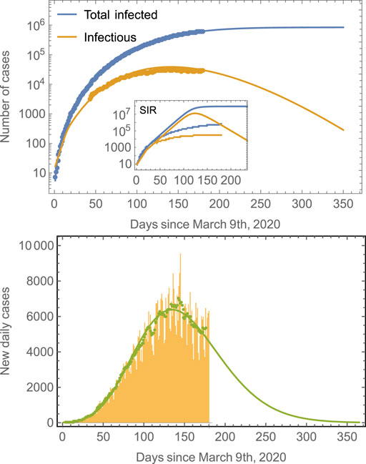
FIGURE 1. Number of cases in Mexico compared to model predictions. The total number of cases (blue line) is obtained from fits of the model defined by Eqs 4–11 to real data for Mexico. The prediction of the number of infectious individuals and of the new daily cases is obtained as a consequence; no independent fittings are required. The model predicts that the peak time for the number of infectious cases is around July 29, 2020, whereas that for the new daily cases is around July 22, 2020. The number of total infected saturates at around 850,000. Note that it is a common trend in epidemiological models to fail longtime predictions [18, 33], and many cases tend to underestimate final observations. Predictions improve as the number of data points considered in the fitting increases. The inset shows the results of a traditional SIR model. The green symbols in the second panel correspond to seven-day averages of the new daily cases data represented by the yellow bars. The green line is the prediction of the model.

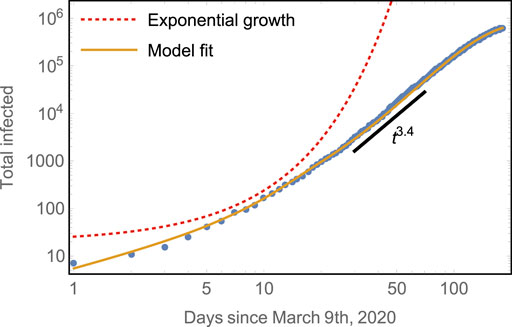
FIGURE 2. Early subexponential growth of the total number of cases compared to model predictions. The model captures both well: the initial exponential rise of total infected and the subsequent algebraic growth with scaling $\simeq t^{3.4}$. An example of exponential growth is shown for comparison.

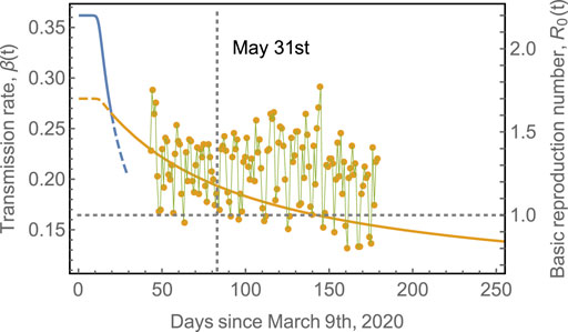
FIGURE 3. Transmission rate, $\beta \left(t\right)$, and time-dependent basic reproduction number $R_0\left(t\right)\equiv \beta \left(t\right)/\gamma$. Two different sections of the transmission rate as a direct consequence of containment policies are obtained. The initial blue section corresponds to a situation in which no specific policy was considered and the spread proceeds without restrictions. The yellow line is the result of the containment measures, consisting in the closure of nonessential activities and the suggestion to stay at home starting from April 1st. The time-dependence of $\beta \left(t\right)$ is not due to the containment policies but is a natural consequence of the asynchronicity of the subpopulation spreads. However, once containment measures were adopted, the basic initial reproduction number decreased from $R_0(t=0)=2.2$ to around $R_0(t=0)\simeq 1.7$. The symbols are obtained from Eq. 4 using real data for Mexico. The dashed vertical line marks the end of the generalized voluntary quarantine of the population on May 31st. The recovery rate was $\gamma =1/6$.

Since the first outbreak of COVID-19 in Mexico remains in progress (at the time of writing this manuscript), it is interesting to evaluate the performance of the model in countries where the first outbreak has nearly ended. We have chosen the eight European countries with the largest number of COVID-19 cases to further validate the model [38]. Figure 4 shows the epidemic curves for Belgium, Italy, France, Germany, Netherlands, Spain, Sweden, and United Kingdom. The model-fits capture the epidemic progression surprisingly well in all cases in spite of the different mitigation strategies applied by each country [39, 40]. Note that the fit starts to fail around $t>80$ particularly in the case of Sweden where a second wave is already apparent. This is due to the fact that we have not taken into consideration the progressive release of the containment measures once the first outbreak has mostly finished. If a larger value for $R_0$ is used around $t=80$, then an increase of the epidemic curve can be obtained again, giving rise to a second wave. In Figure 4, we have used the present model to fit only the first wave in all cases.

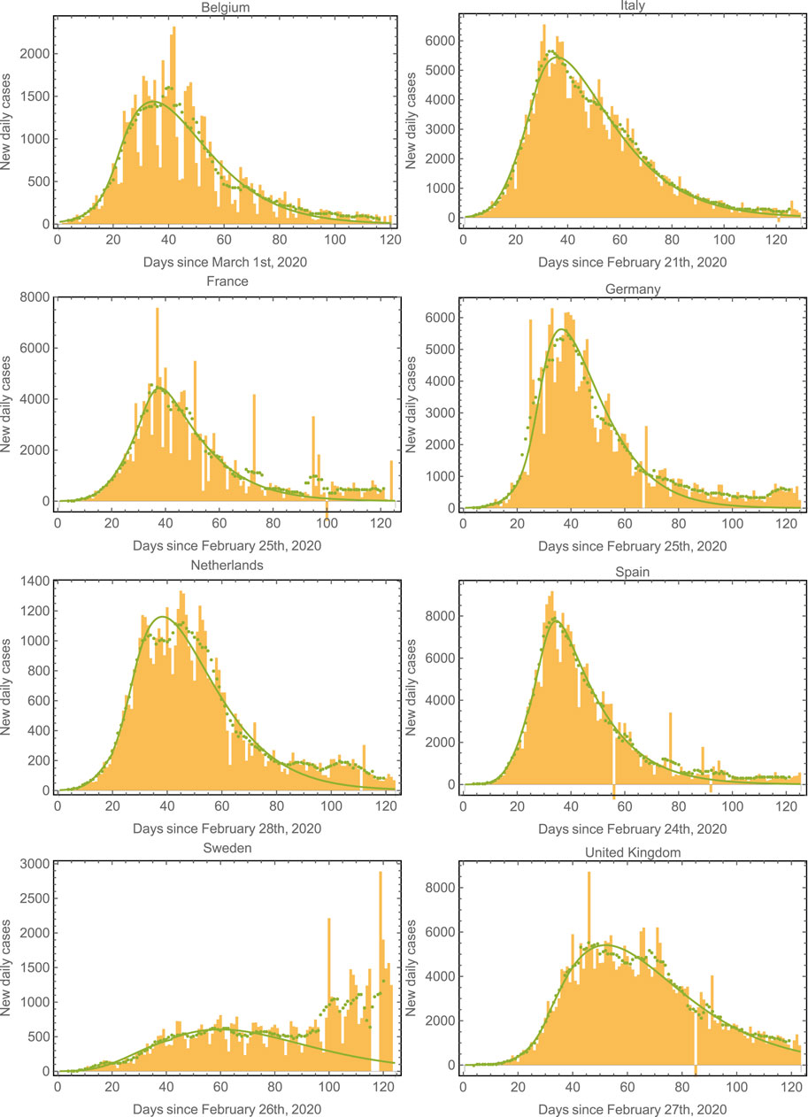
FIGURE 4. Epidemic curves for various countries. We plot the data and model fits for the new daily cases for the eight European countries with the largest number of cases. The model fits correctly capture the epidemic progression in all cases. The green symbols correspond to seven-day averages of the data represented by the yellow bars. Note that the second wave (already apparent in the case of Sweden) could also be fit by considering a third regime with an increased value of $R_0$ due to the gradual release of containment measures starting around $t=80$ days.

Table 1 shows the parameters used to fit the model in Figure 4. In most of these countries, containment measures were taken at about 20–40 days after time $t=0$ days, and thus, the epidemic curve can be divided into two sections, one before and one after the containment measures were adopted. The negative values of $t_0$ found in the first section, before mitigation measures were adopted, reflect the fact that a fraction of the subpopulations whose local outbreaks had not started contributes to the average in Eq. 11. On the other hand, the positive values of $t_0$ in the second section reflect the fact that when confinement measures were adopted, there were already a considerable number of infected individuals. Since the local epidemics in this second section evolve with an assumed attenuated value $R_0$, then, in order to produce the same number of initial cases (which in reality were obtained with the original larger value $R_0$), larger times ($t_0>0$) are needed in the SIR subsystems appearing in Eq. 11. In contrast, the case of Mexico shows a negative value of $t_0$ after the containment measures were adopted, reflecting the fact that the measures were taken very soon in the epidemic progression, when very few cases were present. This is also consistent with the fact that the evolution of the outbreak is taking considerably longer in Mexico than in most of the other countries analyzed. In most cases, the value $\gamma =1/6$ was used as a parameter and the rest of the parameters were obtained by a least-squares fit. We cannot disregard that other choices for the parameter γ could also produce good fits but with different values for the rest of the fit parameters. Additionally, the fact that we are ignoring the incubation time of the disease may give rise to modified fit parameters; thus, they should be considered only as rough estimates.

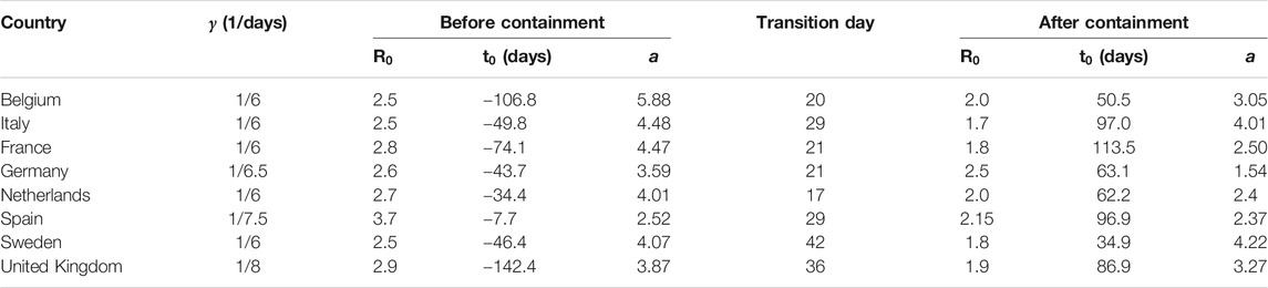
TABLE 1. Fitting parameters used in Figure 4. The effects of containment measures were started to be observed at times $t\simeq 20-40$ days (labeled transition day). Parameters are rough estimates and should not be considered as accurate values.

The effect of the strength of asynchronicity is shown in Figure 5, which shows the evolution of the total number of infected, considering different values for the parameter a, for a given $R_0$. We observe that the longtime total number of infected individuals will be highly dependent on a. The blue line corresponds to the fitted value of a for the case of Mexico, while the yellow and green lines are the predictions for a smaller (smaller a) or a larger (larger a) asynchronicity.

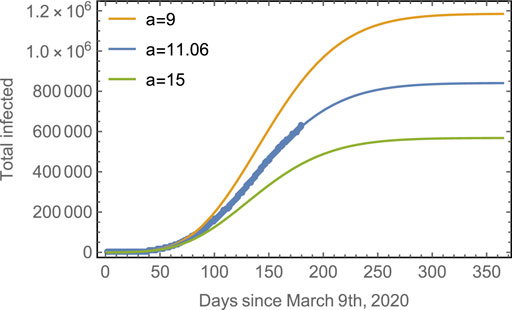
FIGURE 5. Progression of the spread assuming different asynchronicities. Blue line: The observed data points for the total number of cases in Mexico with the fitted model. Yellow line: The predicted evolution for subpopulations with a smaller asynchronicity ($a=9$). Green line: The predicted evolution for subpopulations with a larger asynchronicity ($a=15$). In all cases, $R_0=1.7$ and $\gamma =1/6$.

4 Discussion and Conclusion

Summarizing, we have shown that the spread of the local outbreak onset times and transmission rates can be incorporated in an SIR formulation through the use of a time-dependent basic reproduction number. This quantity is obtained as a solution of the dynamical equations and not introduced externally. Thus, its time-dependence does not arise as a result of changes in the social behavior in response to containment measures or of the depletion of susceptible individuals. Instead, it is the result of an inhomogeneous transmission expressed as a time-dependent average of asynchronic SIR subpopulations (Eq. 11). We have shown that a simple assumption for the distribution of onset times and transmission rates can be at the origin of the algebraic growth observed at the early stages of the COVID-19 outbreak. This contradicts the common assumption that the early growth phase should be exponential in the absence of susceptible depletion or interventional measures. In the present model, containment measures contribute by decreasing the initial reproduction number or equivalently, the initial transmission rate. Other epidemic outbreaks also show early subexponential growth, and a number of potential mechanisms have been proposed to explain it. Among them are the spatial heterogeneity and clustering of contacts arising from the fact that the number of noninfected individuals in the immediate neighborhood of infecting agents is strongly constrained [41, 42]. Reactive population behavior has also been proposed to explain the changes that can gradually mitigate the transmission rate [16, 26, 31, 35–37, 43]. Related to these mechanisms, a range of mechanistic models that can reproduce the subexponential growth dynamics before susceptible depletion sets in have been proposed. These include models with gradually declining contact rate over time [14] and spatially structured models such as household-community networks [26], among others. However, for real epidemics, the underlying mechanisms governing the subexponential growth have been difficult to disentangle, and the matter remains debated [26, 41, 44].

The model predicts a final number of cumulated cases that is substantially smaller than that predicted for homogenous well-mixed populations in agreement with models that predict smaller disease-induced herd immunity when population heterogeneity is taken into account [19].

The present model was validated using the case of the COVID-19 outbreak in different countries, with an emphasis in the case of Mexico. As of the origin of the inhomogeneities in the transmission rates and onset times, one can propose different underlying mechanisms, including the transmission between geographical dispersal subpopulations as individuals travel among them [6, 8, 15]. Another possible source of inhomogeneities is the existence of different social cohorts, with transmission rates between them that are lower than those between individuals of the same cohort [19, 45]. In general, the overall connectivity between subpopulations will determine to a large extent the rate of propagation of the viral agent and the final number of cases. Subpopulations more efficiently connected between them will have smaller dispersion of onset times and transmission rates.

The model is consistent with mitigation strategies, consisting in the design of containment mechanisms oriented to increase inhomogeneities, for example, imposing travel restrictions for long-distance routes, partially isolating subpopulations from each other [46, 47], or by increasing the time an individual takes to move from one subpopulation to the other. Furthermore, travel restrictions could be targeted to highly connected individuals. The reason is that the effective number of susceptible individuals, $s_{eff}\left(t\right)$, that are the responsible for the rate of change of $s\left(t\right)$, decreases with the implementation of such mitigation mechanisms. For countries where a strict quarantine is impracticable, this could be a more realistic alternative. We believe that the insight obtained from the present model may be useful for planning non-pharmaceutical responses to better mitigate or block the overall spread of an epidemic outbreak.

5 Materials and Methods

Identifying the first infectious case is a difficult task, so considering $t=0$ days as the day the first case was reported, does not seem to be appropriate. For this reason, before trying to fit the original data points, we first shifted them in time so that the time $t=0$ days corresponds to the point where a discernible regular behavior starts to appear. This is shown in Supplementary Figure S1 where the data for Mexico that were disregarded for fitting purposes correspond to dates ranging from February 27th, the day of the first detected case, until March 9th. Those data show an irregular behavior probably due to the fewer number of cases and large relative fluctuations.

From a practical point of view, it is numerically easier to approximate $s_{SIR}\left(t\right)$ in Eq. 11 by the function

where the parameters c, q, ν, and τ are obtained from the fitting to the exact form for $s_{SIR}\left(t\right)$ once ${\beta }_0$ and γ are known. The initial conditions $s_{SIR}\left(0\right)=1-1/N_i$, $i_{SIR}\left(0\right)=1/N_i$, and $r_{SIR}\left(0\right)=0$ were assumed. Supplementary Figure S2 shows an example for $s_{SIR}\left(t\right)$ as obtained from the standard SIR model (solid line) and its approximation Eq. 12 (dashed line). By incorporating Eq. 12 into Eq. 11 and the last result into Eqs 4–7, the evolution of $s\left(t\right)$, $i\left(t\right)$, and $r\left(t\right)$ for the whole population is finally obtained.

The fitting of the model to the data, before containment measures were taken, was done choosing the value of a spline function that softens the data taken arbitrarily at time $t=4$ days as an initial condition, as shown in Supplementary Figure S3. In this way, possible misfitting due to fluctuations of the data at the very first data points is minimized. The fitting of the second section of the model, that is, once containment measures were taken at day 20 in the case of Mexico, considered as initial values of the model, the values obtained from the first section evaluated at day 20.

For the case of Mexico, the parameters used were $R_0=2.2$ and $\gamma =1/6$, values generally accepted for the initial regime without containment measures, and $R_0=1.7$ for the second regime after containment measures were adopted. The first fitting process considered the first data points up to $t=20$ days with obtained fitting parameters $t_0\simeq -26.8$ days and $a\simeq 6.5$. Analogously, the fitting for the second regime consisted of data from $t=21$ days to the last data point available. For this second regime, the obtained fitting values were $t_0\simeq -896$ days and $a\simeq 11$. The results were largely insensitive to variations in the exact day of transition between the two regimes.

Data Availability Statement

Publicly available datasets were analyzed in this study. These data can be found here: Mexican Government data files. https://covid19.sinave.gob.mx Our World in Data. https://ourworldindata.org/coronavirus.

Author Contributions

CM conceived the research, developed the mathematical model, wrote the manuscript, and approved the submitted version.

Funding

Partial financial support was provided by DGAPA-UNAM through grant DGAPA IN-103419.

Conflict of Interest

The author declares that the research was conducted in the absence of any commercial or financial relationships that could be construed as a potential conflict of interest.

Acknowledgments

The author thanks Oleg Kogan, David Reguera, and Juan Adrián Reyes for their fruitful discussions and helpful comments.

Supplementary Material

The Supplementary Material for this article can be found online at: https://www.frontiersin.org/articles/10.3389/fphy.2021.683364/full#supplementary-material

References

1. Tian H, Liu Y, Li Y, Wu C-H, Chen B, Kraemer MUG, et al. An Investigation of Transmission Control Measures during the First 50 Days of the COVID-19 Epidemic in China. Science (2020) 368:638. doi:10.1126/science.abb6105
2. Sun G-Q, Wang S-F, Li M-T, Li L, Zhang J, Zhang W, et al. Transmission Dynamics of COVID-19 in Wuhan, China: Effects of Lockdown and Medical Resources. Nonlinear Dyn (2020) 101:1981. doi:10.1007/s11071-020-05770-9
3. Giordano G, Blanchini F, Bruno R, Colaneri P, Di Filippo A, Di Matteo A, et al. Modelling the COVID-19 Epidemic and Implementation of Population-wide Interventions in Italy. Nat Med (2020) 26:855. doi:10.1038/s41591-020-0883-7
4. Walker PGT, Whittaker C, Watson OJ, Baguelin M, Winskill P, Hamlet A, et al. The Impact of COVID-19 and Strategies for Mitigation and Suppression in Low- and Middle-Income Countries. Science (2020) 369:413. doi:10.1126/science.abc0035
5. López L, Rodó X. The End of Social Confinement and COVID-19 Re-emergence Risk. Nat Hum Behav (2020) 4:746. doi:10.1038/s41562-020-0908-8
6. Danon L, House T, Keeling MJ. The Role of Routine versus Random Movements on the Spread of Disease in Great Britain. Epidemics (2009) 1:250. doi:10.1016/j.epidem.2009.11.002
7. Fitzpatrick MC, Bauch CT, Townsend JP, Galvani AP. Modelling Microbial Infection to Address Global Health Challenges. Nat Microbiol (2019) 4:1612. doi:10.1038/s41564-019-0565-8
8. Riley S. Large-Scale Spatial-Transmission Models of Infectious Disease. Science (2007) 316:1298. doi:10.1126/science.1134695
9. Chinazzi M, Davis JT, Ajelli M, Gioannini C, Litvinova M, Merler S, et al. The Effect of Travel Restrictions on the Spread of the 2019 Novel Coronavirus (COVID-19) Outbreak. Science (2020) 368:395. doi:10.1126/science.aba9757
10. Koo JR, Cook AR, Park M, Sun Y, Sun H, Lim JT, et al. Interventions to Mitigate Early Spread of SARS-CoV-2 in Singapore: a Modeling Study. Lancet Infect Dis (2020) 20:678. doi:10.1016/s1473-3099(20)30162-6
11. Nimmagadda V, Kogan O, Khain E. Path-dependent Course of Epidemic: Are Two Phases of Quarantine Better Than One? EPL (Europhysics Letters) (2020) 132:28003. doi:10.1209/0295-5075/132/28003
12. Kermack WO, McKendrick AG. Contributions to the Mathematical Theory of Epidemics–I. 1927. Bull Math Biol (1991) 53:33. doi:10.1016/s0092-8240(05)80040-0
13. Siettos CI, Russo L. Mathematical Modeling of Infectious Disease Dynamics. Virulence (2013) 4:295. doi:10.4161/viru.24041
14. Chowell G, Sattenspiel L, Bansal S, Viboud C. Mathematical Models to Characterize Early Epidemic Growth: A Review. Phys Life Rev (2016) 18:66. doi:10.1016/j.plrev.2016.07.005
15. Hufnagel L, Brockmann D, Geisel T. Forecast and Control of Epidemics in a Globalized World. PNAS (2004) 101:15124. doi:10.1073/pnas.0308344101
16. Maier BF, Brockmann D. Effective Containment Explains Subexponential Growth in Recent Confirmed COVID-19 Cases in China. Science (2020) 368:742. doi:10.1126/science.abb4557
17. Blasius B. Power-law Distribution in the Number of Confirmed COVID-19 Cases. Chaos (2020) 30:093123. doi:10.1063/5.0013031
18. Mena RH, Velasco-Hernandez JX, Mantilla-Beniers NB, Carranco-Sapiéns GA, Benet L, Boyer D, et al. Using Posterior Predictive Distributions to Analyse Epidemic Models: COVID-19 in Mexico City. Phys Biol (2020) 17:065001. doi:10.1088/1478-3975/abb115
19. Britton T, Ball F, Trapman P. A Mathematical Model Reveals the Influence of Population Heterogeneity on Herd Immunity to SARS-CoV-2. Science (2020) 369:846. doi:10.1126/science.abc6810
20. Blyuss KB, Kyrychko YN. Effects of Latency and Age Structure on the Dynamics and Containment of COVID-19. J Theor Biol (2021) 513:110587. doi:10.1016/j.jtbi.2021.110587
21. Ndaïrou F, Area I, Nieto JJ, Torres DFM. Mathematical Modeling of COVID-19 Transmission Dynamics with a Case Study of Wuhan, Chaos, Solitons & Fractals (2020) 135: 109846. Corrigendum Chaos, Solitons & Fractals (2020) 141:110311. doi:10.1016/j.chaos.2020.110311
22. Ajelli M, Fumanelli L, Manfredi P, Merler S. Spatiotemporal Dynamics of Viral Hepatitis A in Italy. Theor Popul Biol (2011) 79:1. doi:10.1016/j.tpb.2010.09.003
23. Sattenspiel L. The Geographic Spread of Infectious Diseases: Models and Applications. New Jersey: Princeton University Press (2009).
24. Ball F, Britton T, House T, Isham V, Mollison D, Pellis L, et al. Seven Challenges for Metapopulation Models of Epidemics, Includinghouseholds Models. Epidemics (2015) 10:63. doi:10.1016/j.epidem.2014.08.001
25. Li Q, Guan X, Wu P, Wang X, Zhou L, Tong Y, et al. Early Transmission Dynamics inWuhan, China, of Novel Coronavirus-Infected Pneumonia. The New Engl J Med a (2020) 382:1199. doi:10.1056/nejmoa2001316
26. Chowell G, Viboud C, Simonsen L, Moghadas SM. Characterizing the Reproduction Number of Epidemics with Early Subexponential Growth Dynamics. J R Soc Interf (2016) 13:20160659. doi:10.1098/rsif.2016.0659
27. Lloyd AL, May RM. Spatial Heterogeneity in Epidemic Models. J Theor Biol (1996) 179:1. doi:10.1006/jtbi.1996.0042
28. Keeling MJ, Rohani P. Estimating Spatial Coupling in Epidemiological Systems: a Mechanistic Approach. Ecol Lett (2002) 5:20. doi:10.1046/j.1461-0248.2002.00268.x
29. Lloyd AL, Jansen VAA. Spatiotemporal Dynamics of Epidemics: Synchrony in Metapopulation Models. Math Biosciences (2004) 188:1. doi:10.1016/j.mbs.2003.09.003
30. Chen Y-C, Lu P-E, Chang C-S, Liu T-H. A Time-dependent SIR Model for COVID-19 with Undetectable Infected Persons. IEEE Trans Netw Sci Eng (2020) 7:3279. doi:10.1109/tnse.2020.3024723
31. Caccavo D. Chinese and Italian COVID-19 Outbreaks Can Be Correctly Described by a Modified SIRD Model. New Haven: Yale University (2020). doi:10.1101/2020.03.19.20039388
32.Mexican Government data files. https://covid19.sinave.gob.mx
33. Castro M, Ares S, Cuesta JA, Manrubia S. The Turning point and End of an Expanding Epidemic Cannot Be Precisely Forecast. PNAS (2020) 117:26190. doi:10.1073/pnas.2007868117
34. Li ML, Overview of DELPHI Model V2.0. (2020) https://www.covidanalytics.io/DELPHI_documentation_pdf
35. Funka S, Gilad E, Watkins C, Jansen VAA. The Spread of Awareness and its Impact on Epidemic Outbreaks. Proc Natl Acad Sci (2009) 106:6872. doi:10.1073/pnas.0810762106
36. Wang Z, Guo Q, Sun S, Xia C. The Impact of Awareness Diffusion on SIR-like Epidemics in Multiplex Networks. Appl Math Comput (2019) 349:134. doi:10.1016/j.amc.2018.12.045
37. Wang Z, Xia C, Chen Z, Chen G. Epidemic Propagation with Positive and Negative Preventive Information in Multiplex Networks. IEEE Trans Cybernetics (2021) 51:1454. doi:10.1109/tcyb.2019.2960605
38.Our World in Data. https://ourworldindata.org/coronavirus
39. Flaxman S, Mishra S, Gandy A, Unwin HJT, Mellan TA, Coupland H, et al. Estimating the Effects of Non-pharmaceutical Interventions on COVID-19 in Europe. Nature (2020) 584:257. doi:10.1038/s41586-020-2405-7
40. Cheng C, Barceló J, Hartnett AS, Kubinec R, Messerschmidt L. COVID-19 Government Response Event Dataset (CoronaNet v.1.0). Nat Hum Behav (2020) 4:756. doi:10.1038/s41562-020-0909-7
41. Kiskowski M, Chowell G. Modeling Household and Community Transmission of Ebola Virus Disease: Epidemic Growth, Spatial Dynamics and Insights for Epidemic Control. Virulence (2016) 7:163. doi:10.1080/21505594.2015.1076613
42. Szendrói B, Csányi G. Polynomial Epidemics and Clustering in Contact Networks. Proc R Soc Lond B (Suppl (2004) 271:S364. doi:10.1098/rsbl.2004.0188
43. Viboud C, Simonsen L, Chowell G. A Generalized-Growth Model to Characterize the Early Ascending Phase of Infectious Disease Outbreaks. Epidemics (2016) 15:27. doi:10.1016/j.epidem.2016.01.002
44. Chowell G, Viboud C, Hyman JM, Simonsen L, The Western Africa Ebola Virus Disease Epidemic Exhibits Both Global Exponential and Local Polynomial Growth Rates, PLoS Currents Outbreaks Jan 21, 1 (2015). doi:10.1371/currents.outbreaks.8b55f4bad99ac5c5db3663e916803261
45. Khain E. Two-level Modeling of Quarantine. Phys Rev E (2020) 102:022313. doi:10.1103/PhysRevE.102.022313
46. Li M-T, Sun G-Q, Zhang J, Zhao Y, Pei X, Li L, et al. Analysis of COVID-19 Transmission in Shanxi Province with Discrete Time Imported Cases. Math Biosciences Engeneering (2020) 17:3710. doi:10.3934/mbe.2020208
Keywords: COVID-19, SARS-CoV-2, mathematical modeling, compartmental models, susceptible-infected-recovered model, forecasting
Citation: Mendoza CI (2021) Inhomogeneous Transmission and Asynchronic Mixing in the Spread of COVID-19 Epidemics. Front. Phys. 9:683364. doi: 10.3389/fphy.2021.683364
Received: 20 March 2021; Accepted: 24 May 2021;
Published: 15 June 2021.
Edited by:
Hui-Jia Li, Beijing University of Posts and Telecommunications (BUPT), ChinaReviewed by:
Chengyi Xia, Tianjin University of Technology, ChinaGui-Quan Sun, North University of China, China
Copyright © 2021 Mendoza. This is an open-access article distributed under the terms of the Creative Commons Attribution License (CC BY). The use, distribution or reproduction in other forums is permitted, provided the original author(s) and the copyright owner(s) are credited and that the original publication in this journal is cited, in accordance with accepted academic practice. No use, distribution or reproduction is permitted which does not comply with these terms.
*Correspondence: Carlos I. Mendoza, cmendoza@materiales.unam.mx