2.1 Site and instrumentation

Field measurements were conducted at the Dianshan Lake (DSL) site (31.096^∘ N, 120.988^∘ E; 14 m a.g.l. – meters above ground level) at the junction of the Shanghai, Zhejiang, and Jiangsu provinces of the Yangtze River Delta (YRD) region of China (Fig. S1 in the Supplement). It represents a rural setting and the regional-scale air pollution characteristics of the YRD region. A detailed description of the site can be found in our previous works (Qin et al., 2019, 2020).

Ambient GEM concentration was measured by an automated mercury vapor analyzer (Tekran 2537B/1130/1135 system; Tekran Instruments Corporation, Canada) at a 5 min time resolution. More details on this instrument can be found elsewhere (Qin et al., 2019). Water-soluble ions in PM_2.5 (SO${}_{\mathrm{4}}^{\mathrm{2}-}$, NO${}_{\mathrm{3}}^{-}$, NH${}_{\mathrm{4}}^{+}$, Cl⁻, Na⁺, K⁺, Mg²⁺, and Ca²⁺) and water-soluble gases (NH₃ and SO₂) were continuously measured by the Monitor for AeRosols and Gases in ambient Air (MARGA) at a flow rate of 16.7 L min⁻¹, with a time resolution of 1 h (Wang et al., 2022b; Xu et al., 2020). Heavy metals in PM_2.5 (Pb, Fe, Ba, Cr, Se, Cd, Ag, Ca, Mn, Cu, As, Ni, Zn, and V) were determined hourly by a multi-metal monitor (Xact^™ 625; Cooper Environmental Services, LLC, USA; Wang et al., 2022a). Black carbon in PM_2.5 was continuously measured by a multi-wavelength Aethalometer (AE33, Magee Scientific, USA; Li et al., 2021). Organic carbon (OC) and elemental carbon (EC) in PM_2.5 were measured by an in situ semi-continuous organic carbon and elemental carbon aerosol analyzer (RT-3195; Sunset Laboratory Inc., Beaverton, Oregon, USA; Xu et al., 2018). SO₂, CO, O₃, and PM_2.5 were determined by Thermo Scientific models 43i, 48i-TLE, 49i, and 1405-F, respectively. Meteorological parameters, including air temperature, relative humidity, wind speed, and wind direction, were collected by using a series of Vaisala weather sensors (WXT530 Weather Transmitter Series; Vaisala, Vantaa, Finland) with a time resolution of 10 min.

The air pollutants, including CO, NO₂, and PM_2.5 at other ground monitoring stations in the YRD region were obtained from the public database of the China National Environmental Monitoring Center.

The data of the planetary boundary layer (PBL) height were obtained from the U.S. National Oceanic and Atmospheric Administration (https://www.ready.noaa.gov/archives.php, last access: 31 August 2022). The 3 d air mass backward trajectories were calculated by applying the Hybrid Single-Particle Lagrangian Integrated Trajectory (HYSPLIT) model (https://www.ready.noaa.gov/HYSPLIT.php, last access: 31 August 2022), and MeteoInfo software was used to perform cluster analysis of backward trajectories.

2.2 Machine learning model

The artificial neural network (ANN) model was used to simulate the GEM concentration at the DSL site during the study period. An artificial neural network is a mathematical model based on the basic principles of neural networks in biology. The network structure consists of the input layer, hidden layer, and output layer of neurons. The process of obtaining an ANN model is that the neurons of input layer pass through each hidden layer and then reach the output layer. If the expected results are not obtained in the output layer, then the errors are propagated back, and the neuron weights of each hidden layer are iteratively updated to minimize them. In this study, the long-term observational air pollutants (SO₂, CO, O₃, NO₂, and PM_2.5) and meteorological data (air temperature, relative humidity, and wind speed) in Shanghai from 1 March 2015 to 28 February 2019 were chosen as input variables for training. These variables were directly or indirectly related to the emissions (both anthropogenic and natural sources), transport, and removal processes of GEM. For example, the main sources of SO₂, CO, and NO₂ were fossil fuel combustions, which were also the largest anthropogenic sources of GEM (Zhang et al., 2016a; Streets et al., 2011). The natural sources of GEM were mainly from the release of land and sea surfaces, which were closely related to temperature, relative humidity, and wind speed (Wang et al., 2014; Moore and Carpi, 2005).

The detailed training and validation of this model can be found in our previous study (Qin et al., 2022). We have established an ANN model through training the long-term observational data of GEM and other auxiliary environmental parameters at DSL. The long-term observational GEM (hourly data from 1 March 2015 to 28 February 2019; n=17 532) in Shanghai was the target variable for training, and the corresponding air pollutants (SO₂, CO, O₃, NO₂, and PM_2.5) and meteorological data (air temperature, relative humidity, and wind speed) were chosen as input variables for training. The data sets were randomly divided into three parts, i.e., 70 % for training, 15 % for validation, and 15 % for testing. We chose the neural network containing a hidden layer with 20 nodes, and the training algorithm was the Levenberg–Marquardt. The performance of the model was evaluated with the mean square error (MSE) and correlation coefficient (R² value). To verify the accuracy of the trained neural network model, we compared the observed (not included in the training data set) and simulated GEM concentrations of DSL from 1 January to 26 February 2020 and found that they exhibited a reasonably good correlation with the correlation coefficient (R²) of 0.67. To test the applicability of the model on the regional scale, we compared the observed and simulated GEM concentrations in Suzhou, Ningbo, Nanjing, and Hefei (Fig. S2). In Nanjing and Suzhou, the observed and simulated daily GEM were consistent, with R² values of 0.52 and 0.71, respectively. In Ningbo, the observed and simulated GEM in summer and winter were also consistent, with R² values of 0.64 and 0.65, respectively. A low bias was derived between the observed and simulated seasonal GEM in Hefei. This suggested that it was feasible to use the trained ANN model to simulate the GEM concentrations in Shanghai and even the Yangtze River Delta region.

2.3 SHapley Additive exPlanations (SHAP) approach

The SHAP approach was applied in this study to explain the ANN model simulation results. This approach constructs a distribution scheme based on the coalitional game theory that comprehensively considers the requirements of the conflicting parties, so as to ensure the fairness of the distribution (Lundberg et al., 2018, 2020; Hou et al., 2022). In the game theory, the Shapley value of a player represents the average contribution of the player in a cooperative game, which is a fair distribution of the total gain generated by individual players (Lundberg and Lee, 2017). In the context of machine learning prediction, the Shapley value of a feature at a query point represents the contribution of that feature to the prediction (response for regression or score of each class for classification) at a particular query point (Aas et al., 2021). The Shapley value corresponds to the deviation between the prediction for the query point and the average prediction caused by the feature, and the sum of the Shapley values for all features for specific query point corresponds to the total deviation of the prediction from the average (Kumar et al., 2020). The Shapley value of the ith feature for the query point x is defined by the value function v as follows:

where N is the number of all features, ω is the set of all features, |S| is the cardinality of the set S or the number of elements in the set S, and v_x is the value function of the features in a set S for the query point x. The value of the function indicates the expected contribution of the features in S to the prediction for the query point x.

2.4 Positive matrix factorization (PMF)

The PMF model has proven to be a useful tool for obtaining source profiles and quantifying source contributions of complex air pollution (Gibson et al., 2015). The basic principle of PMF is that the concentration of the sample is determined by the source profiles with different contributions, which can be described as follows:

where X_ij represents the concentration of the jth species in the ith sample, g_ik is the contribution of the kth factor in the ith sample, f_kj provides the information about the mass fraction of the jth species in the kth factor, e_ij is the residual for specific measurement, and P represents the number of factors. The number of factors being from three to eight was explored, with the optimal solutions determined by the slope of the Q value versus the number of factors. The Q value is the sum of the square of the difference between the measured and modeled concentrations weighted by the concentration uncertainties and needs to be minimized before the PMF modeled determines the optimal nonnegative factor profiles and contributions (Cheng et al., 2015).

where X_ij represents the concentration of the jth contamination in the ith sample, m is the total number of the pollutants, and n is the total number of samples. A_ik represents the contribution of the kth factor on the ith sample, and F_kj represents the mass fraction of the j pollutant in the kth factor. S_ij is the uncertainty in the jth pollutant on the ith factor, and P is the number of factors. For each run in this study, the stability and reliability of the outputs were assessed by referring to the Q value, residual analysis, and correlation coefficients between observed and predicted concentrations. Finally, we found that a six-factor solution showed the most stable results and gave the most reasonable interpretation. A detailed description can be seen in previous studies (Qin et al., 2020, 2019).

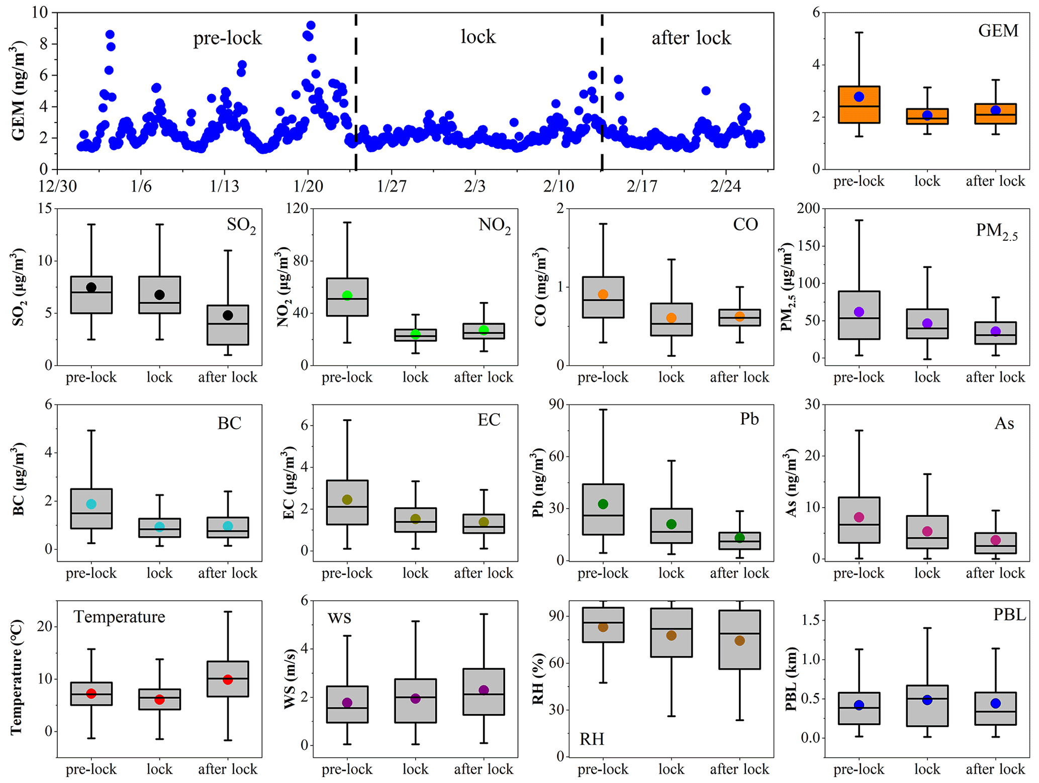
Figure 1Hourly variations in GEM concentrations from 1 January to 26 February 2020. Box plots of GEM, SO₂, NO₂, CO, PM_2.5, BC, EC, Pb, As, and meteorological parameters (temperature, wind speed, relative humidity, and planetary boundary layer height) before, during, and after the lockdown are also shown.

Download

3.1 Changes in GEM concentrations during the lockdown

Figure 1 shows the time series of hourly GEM concentrations during 1 January to 26 February 2020. Three periods were defined, i.e., 1 to 23 January before the lockdown, 24 January to 14 February during the lockdown, and 15 to 26 February after the lockdown. Before the lockdown, hourly GEM showed strong fluctuations, with frequent extreme concentrations higher than 5 ng m⁻³. In contrast, the diurnal variation in GEM was significantly weakened, with hourly concentrations all lower than 4 ng m⁻³ during the lockdown. After the lockdown, GEM concentration was slightly higher than that of during the lockdown. On average, GEM declined sharply from 2.78 ng m⁻³ before the lockdown to 2.06 ng m⁻³ during the lockdown and then rose slightly to 2.26 ng m⁻³ after the lockdown. Figure 1 also shows that typical gaseous pollutants, such as sulfur dioxide (SO₂), nitrogen dioxide (NO₂), and carbon monoxide (CO), behaved similarly to GEM, in addition to the PM_2.5 and its components such as black carbon (BC), elemental carbon (EC), lead (Pb), and arsenic (As). This temporal pattern was expected, as the nationwide reduction in automotive mobility and energy consumption due to the COVID-19 lockdown would certainly have lead to drops in primary pollutants emissions. As shown in Fig. S3, the levels of CO, NO₂, and PM_2.5 in the Yangtze River Delta (YRD) declined sharply during the lockdown by 26 %, 61 %, and 27 %, respectively, which was consistent with emissions estimates based on up-to-date activity levels in eastern China (Huang et al., 2021). For anthropogenic Hg emissions, one study in the Beijing–Tianjin–Hebei region estimated a decline of approximately 22 % during the lockdown, which was mainly due to the reduction in cement clinker production, coal-fired power plants, and residential coal combustion (Wu et al., 2021). We compared the meteorological factors (including air temperature, wind speed, relative humidity, and planetary boundary layer height) before, during, and after the lockdown (Table S1). No significant changes in the meteorological factors were observed before and during the lockdown. In addition, the 3 d backward trajectory cluster analysis indicated that the transport patterns differed little between these two periods (Fig. S4). This suggested that the significant decline in GEM concentrations during the lockdown was mainly due to the reduced mercury emissions, rather than changes in synoptic conditions.

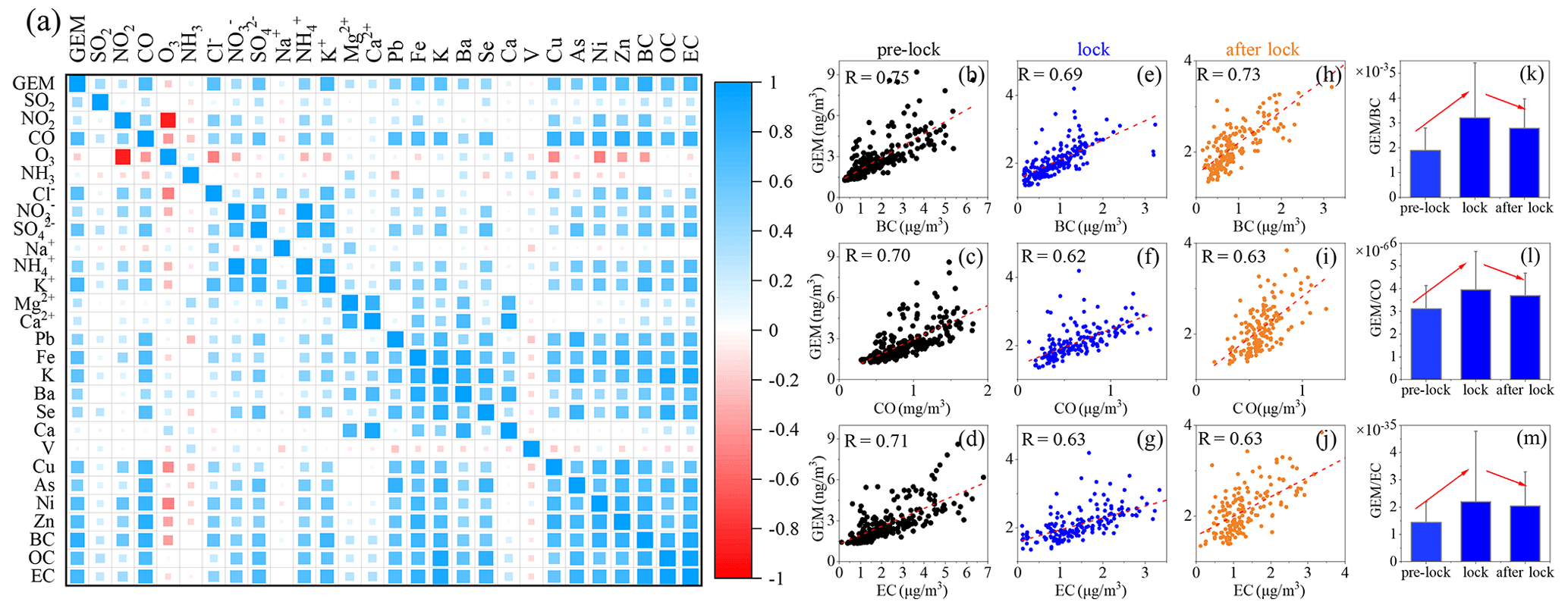
Figure 2(a) Correlation coefficient matrix among GEM and PM_2.5 components and gaseous pollutants during the whole study period. Relationship between GEM and BC, CO, and EC (b–d) before, (e–g) during, and (h–j) after the lockdown. (k–m) The change in $\mathrm{GEM}/\mathrm{BC}$, $\mathrm{GEM}/\mathrm{CO}$, and $\mathrm{GEM}/\mathrm{EC}$ ratios before, during, and after the lockdown.

Download

3.2 Observational evidences of enhanced effects of natural sources on GEM

Table S2 further shows that the reduction rates of gaseous pollutants SO₂, NO₂, NO, and CO during the lockdown were 9 %, 56 %, 64 %, and 33 %, respectively, compared to those before the lockdown, while O₃ showed an almost 1-fold increase due to the strongly depressed titration effect from substantial reduced NO_x emissions during the lockdown (Huang et al., 2021; Yang et al., 2021). As for the primary trace elements such as Pb, Fe, Cr, Se, Ca, Mn, As, Ni, and Zn, their reduction rates ranged from 34 % to 73 %. As for the main chemical components in PM_2.5, NO${}_{\mathrm{3}}^{-}$, NH${}_{\mathrm{4}}^{+}$, and BC were strongly reduced by 58 %, 45 %, and 51 %, while SO${}_{\mathrm{4}}^{\mathrm{2}-}$ and OC were less reduced by 20 % and 16 %, respectively. Except for SO₂, SO${}_{\mathrm{4}}^{\mathrm{2}-}$, and OC, GEM presented a lower reduction rate than the other air pollutants, probably indicating the discrepancy in key sources for different air pollutants. In order to probe the dynamic variation in GEM sources across the observational period, we first investigated the correlations among GEM and main components of PM_2.5 and gaseous pollutants (Fig. 2a). GEM was found to be significantly correlated with the primary air pollutants such as CO, K⁺, BC, and EC, with the correlation coefficients (R) above 0.7. This suggested that the main anthropogenic sources of GEM might be coal combustion and biomass burning in Shanghai, which was consistent with the previous studies in the Yangtze River Delta (Qin et al., 2019; Tang et al., 2018).

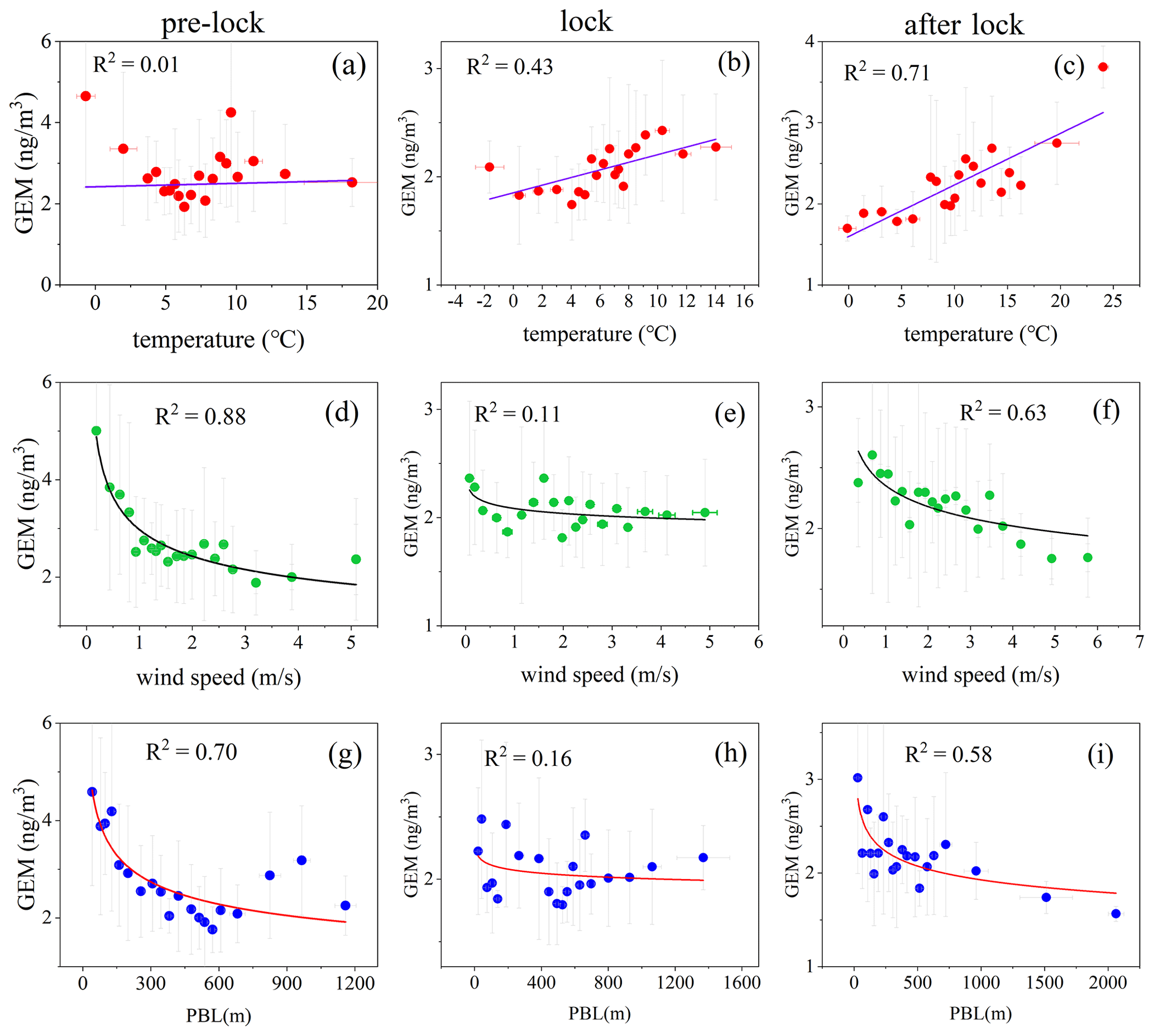
Figure 3Relationship between GEM concentration and (a–c) temperature, (d–f) wind speed, and (g–i) PBL height before, during, and after the lockdown.

Download

BC, EC, and CO are mainly from fossil fuels combustion and biomass burning and can be used as indicators of the main anthropogenic sources of GEM. In order to explore the changes in the sources of GEM, we further investigated the relationship between GEM and BC/EC/CO before, during, and after the lockdown. As shown in Fig. 2, R between GEM and BC, GEM and CO, and GEM and EC during and after the lockdown were lower than that before the lockdown, suggesting the influence of anthropogenic sources on GEM was weakened during the lockdown. Different from BC, CO, and EC, which are overwhelmingly derived from anthropogenic sources, natural sources such as surface emission and ocean release also contribute significantly to GEM (Obrist et al., 2018). Hence, the ratio of $\mathrm{GEM}/\mathrm{BC}$, $\mathrm{GEM}/\mathrm{CO}$, and $\mathrm{GEM}/\mathrm{EC}$ can be simply applied as indicators to reveal the relative importance of anthropogenic versus natural sources. A higher $\mathrm{GEM}/\mathrm{BC}$, $\mathrm{GEM}/\mathrm{CO}$, and $\mathrm{GEM}/\mathrm{EC}$ ratio indicated the greater importance of natural sources, and vice versa. As shown in Fig. 2k–m, the $\mathrm{GEM}/\mathrm{BC}$ ratio significantly increased from $\mathrm{1.9}\times {\mathrm{10}}^{-\mathrm{3}}$ before the lockdown to $\mathrm{3.2}\times {\mathrm{10}}^{-\mathrm{3}}$ during the lockdown, the $\mathrm{GEM}/\mathrm{CO}$ ratio significantly increased from $\mathrm{3.1}\times {\mathrm{10}}^{-\mathrm{6}}$ to $\mathrm{4.0}\times {\mathrm{10}}^{-\mathrm{6}}$, and the $\mathrm{GEM}/\mathrm{EC}$ ratio significantly increased from $\mathrm{1.4}\times {\mathrm{10}}^{-\mathrm{3}}$ to $\mathrm{2.2}\times {\mathrm{10}}^{-\mathrm{3}}$. The $\mathrm{GEM}/\mathrm{CO}$ ratio has been used to analyze the sources of GEM in many studies. In this study, the $\mathrm{GEM}/\mathrm{CO}$ ratio during the lockdown period was $\mathrm{4.0}\times {\mathrm{10}}^{-\mathrm{6}}$, which was significantly higher than the anthropogenic $\mathrm{GEM}/\mathrm{CO}$ emission ratio in mainland China, South Asia, and the Southeast Asian peninsula, whose values were 2.7, 2.6, and $\mathrm{1.5}\times {\mathrm{10}}^{-\mathrm{6}}$, respectively (Fu et al., 2015). These values were also higher than the $\mathrm{GEM}/\mathrm{CO}$ ratio observed in Nanjing ($\mathrm{3.1}\times {\mathrm{10}}^{-\mathrm{6}})$ and Beijing ($\mathrm{1.5}\times {\mathrm{10}}^{-\mathrm{6}})$ in winter (Zhang et al., 2013; Zhu et al., 2012). This corroborated that the impact of natural sources on GEM could be more outstanding during the lockdown than before and after the lockdown.

Previous studies have demonstrated the strong dependence of natural surface emissions on meteorological factors such as temperature, wind speed, and relative humidity (Pannu et al., 2014; Lindberg et al., 2007; Gustin et al., 2005). We compared the relationship between GEM and meteorological parameters before, during, and after the lockdown to investigate the changes in natural sources of mercury. As shown in Fig. 3a–c, there was no clear correlation between GEM and temperature before the lockdown, while moderately high correlations during and after the lockdown emerged with the correlation coefficients (R²) of 0.43 and 0.71, respectively. This might indicate the enhanced role of natural sources on GEM concentrations due to the lockdown control measures. For wind speed (Fig. 3d–f), strongly negative correlations were observed with GEM before and after the lockdown but not during the lockdown. On the one hand, the high wind speed was beneficial to the diffusion of air pollutants in the atmosphere, which explained the negative correlation between GEM and wind speed. On the other hand, the high wind speed promoted the natural surface release of mercury, partially canceling out the diffusion effect of the wind speed, which induced the ambiguous relationship between GEM and wind speed during the lockdown. The relationship between GEM and PBL height was similar to that of wind speed, showing strongly negative correlations before and after the lockdown while having weak correlations during the lockdown (Fig. 3g–i). The increase in PBL height was beneficial to the diffusion of GEM. While the increase in PBL height usually occurred in the daytime when temperature was high, which was conducive to the natural surface release of mercury. Therefore, ambient GEM did not decrease significantly with the increase in PBL height during the lockdown.

Overall, all the observational evidence possibly suggested that the role of natural emissions on GEM was more manifested due to the lockdown. However, all the results were based on qualitative data analysis. In the following sections, the machine learning and source apportionment methods will be applied to quantify the contribution of anthropogenic and natural sources to GEM during the three defined periods.

3.3 Understanding the drivers of GEM variation by explainable machine learning

We further conducted machine learning simulations using the trained artificial neural network (ANN), which has already been established by training the long-term (2015–2019) observational data of GEM and other necessary environmental parameters (including SO₂, NO₂, CO, O₃, PM_2.5, temperature, relative humidity, and wind speed) at the Dianshan Lake site (Qin et al., 2022). Figure 4a–b show the comparison of ANN simulated and observed GEM concentrations during the whole study period and found that their correlation coefficient is acceptable (R²=0.67). As shown in Fig. S5, we examined the performance of the ANN model before, during, and after the lockdown. The correlations between ANN simulated and observed GEM concentrations were also acceptable, with correlation coefficients of 0.67, 0.59, and 0.63, respectively. Then we applied the SHapley Additive exPlanations (SHAP) approach to uncover the mystery of the machine learning “black box” model (see the methods in Sect. 2.3). This approach has the potential to quantify the global and local impacts of input features on model predictions (Lundberg and Lee, 2017), which has been used in various fields (Mangalathu et al., 2020; Hou et al., 2022; Lundberg et al., 2018; Zhong et al., 2021; Wang et al., 2021).

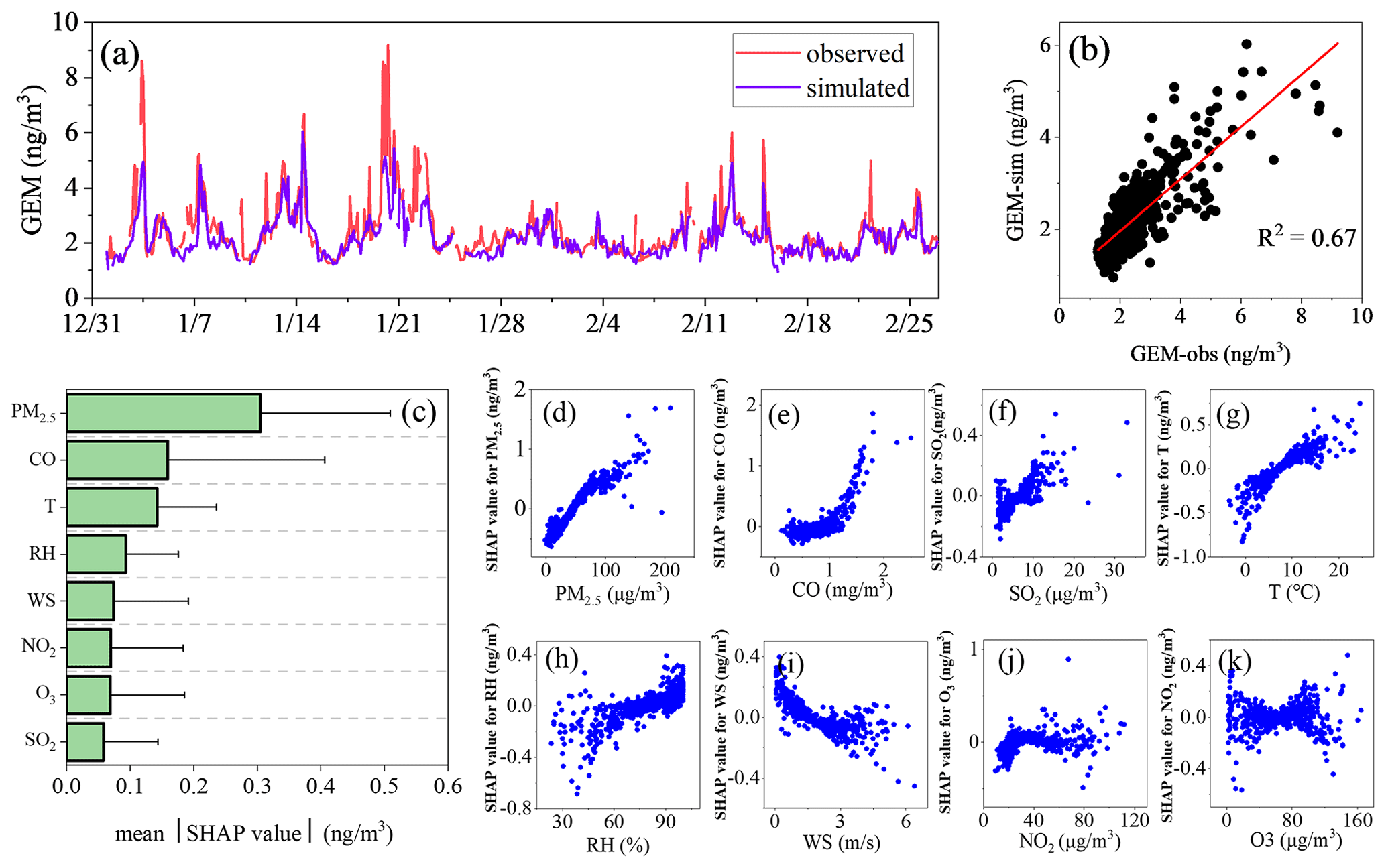
Figure 4(a) Time series of ANN simulated and observed GEM concentrations during the study period. (b) Linear correlation between observed and ANN simulated GEM concentrations. (c) The ranking of input features calculated via the SHAP algorithm. (d–k) Relationship between the SHAP value and the corresponding concentration of each feature.

Download

We calculated the SHAP value of each feature to represent the global importance of the feature, which can be used to indicate the general impact of various features across all samples. As shown in Fig. 4c, by comparing the average absolute SHAP values, PM_2.5 ranked as the most important feature, which changed the simulated GEM concentrations by 0.30±0.20 ng m⁻³, followed by CO and temperature with the SHAP values of 0.16±0.25 and 0.14±0.09 ng m⁻³, respectively. The average values of the remaining factors were less than 0.1 ng m⁻³. We further investigated the relationship between the SHAP value of each feature and its concentration. As shown in Fig. 4d–f, with the increase in PM_2.5, CO, and SO₂ concentrations, their corresponding SHAP values increased accordingly. Previous studies have shown that GEM, PM_2.5, CO, and SO₂ shared common anthropogenic sources, such as the combustion of fossil fuels and biomass (Chong et al., 2019; Fu et al., 2015), thus interpreting the positive effect of various anthropogenic emission sources on GEM. A similar relationship was also found for temperature and relative humidity with their corresponding SHAP values (Fig. 4g–h). Since temperature and relative humidity are important factors affecting the natural release of GEM from natural surfaces (Pannu et al., 2014; Wang et al., 2016), the positive influence of natural surface emissions on GEM was expected. In contrast, the SHAP value of wind speed negatively correlated with the magnitude of wind speed (Fig. 4i), thus indicating the diffusion/accumulation effect of wind speed on GEM. The SHAP values of NO₂ and O₃ did not show obvious correlations with their concentrations (Fig. 4j–k). One of the main sources of NO₂ was vehicle emissions, which contributed little to GEM. As for O₃, its oxidation on GEM was also limited. Thus, neither NO₂ nor O₃ exhibited considerable effects on regulating the GEM variation.

To more explicitly identify the drivers to the dynamic variation in GEM, a process analysis of GEM pollution episodes was conducted. One pollution episode was defined as having its average GEM concentration for more than 35 % of the day before the episode and lasting for more than 3 d. Based on this criterion, two pollution episodes (PE1 and PE2) before the lockdown, one pollution episode (PE3) during the lockdown, and one pollution episode (PE4) after the lockdown were selected (Fig. S6). As shown in Fig. 5, the drivers of the first two pollution episodes were significantly different from the last two. The main influencing factors in PE1 were PM_2.5 and CO, which represented anthropogenic sources, contributing 0.65 and 0.51 ng m⁻³ to the GEM variation, respectively. Similar to PE1, PM_2.5 and CO in PE2 contributed the most to the GEM variation in 0.35 and 0.12 ng m⁻³, respectively. This indicated that the two mercury pollution episodes before the lockdown were mainly driven by anthropogenic sources. In contrast, in PE3 and PE4, temperature ranked the first among all the variables, with a contribution to GEM of 0.10 and 0.14 ng m⁻³, respectively. This suggested that these two pollution episodes during and after the lockdown occurred under the dominance of natural sources.

In addition, we found that there was a tradeoff between the SHAP value of temperature and the SHAP value of PM_2.5 and CO. As shown in Fig. 5b–c, the SHAP value of temperature decreased with the increase in the SHAP value of PM_2.5 and CO throughout the study period. This probably suggests that the increase in anthropogenic GEM emissions may inhibit the release of natural sources to some extent, which will be discussed later.

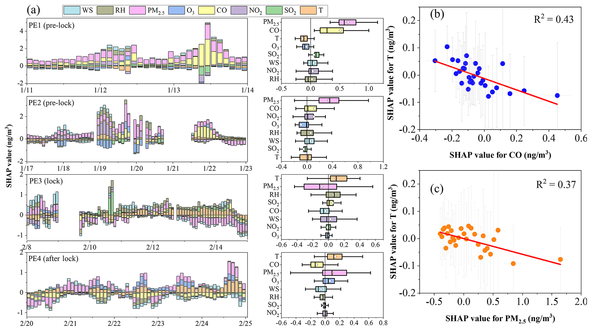
Figure 5(a) Time series and box plots of each feature's SHAP value during the four mercury pollution episodes. (b–c) Relationship between the SHAP value of temperature and SHAP value of CO and PM_2.5 during the whole study period.

Download

3.4 Response of natural release of GEM to the lockdown

To quantify the changes in the contribution of different sources to GEM, we applied the PMF model to analyze the sources of GEM during the whole study period. Figure S7 shows the resolved factors and factor loadings, which were similar to the results by previous study at the same site (Qin et al., 2020). A total of six sources were resolved, namely coal combustion, with high loadings of SO${}_{\mathrm{4}}^{\mathrm{2}-}$, Pb, K⁺, As, and Se, natural surface emissions, with high loadings of temperature and NH₃, vehicle emissions, with high loadings of NO, ship emissions, with high loading of Ni, iron and steel production, with high loadings of Fe, Cr, and Mn, and cement production, with high loading of Ca. The mean contributions of the six factors above to GEM were 55 %, 28 %, 7 %, 5 %, 3 %, and 3 %, respectively (Fig. S7). To evaluate the uncertainty in the PMF results, the Fpeak model run at the strength of 0.5, −0.5, 1, and −1 were conducted by using the rotation tools in PMF. The changes in Q value (dQ) due to the Fpeak rotation were less than 1 % of the base run Q (robust) value (Table S3), which is less than the benchmark value of 5 %. The profiles and contributions of each source were also examined, and there were no significant differences between the factor contributions of the base run and rotation results, especially for coal combustion and natural surface emissions. Hence, the base run results were used in this study.

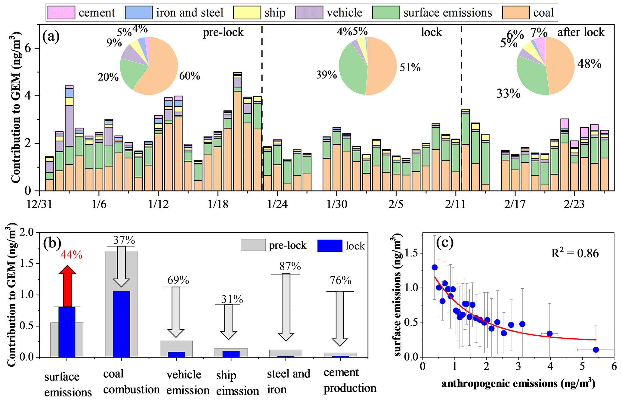
Figure 6(a) Daily average concentrations of apportioned GEM from six sources based on PMF modeling. Pie charts represent the relative contribution of the six sources to GEM during three periods. (b) Changes in the absolute contribution of natural and anthropogenic sources to GEM before and during the lockdown. (c) Relationship between absolute contribution of natural surface emissions and anthropogenic sources to GEM during the whole study period.

Download

Figure 6a shows the time series of apportioned GEM concentrations and relative contributions from six sources during three periods. Significant changes in the sources of GEM were observed due to the lockdown. The contribution of coal combustion fell from 60 % before the lockdown to 51 % during the lockdown and 48 % after the lockdown. On the contrary, the relative contribution of natural surface emissions rose significantly from 20 % before the lockdown to 39 % during the lockdown, and then dropped slightly to 33 % after the lockdown. In addition to the increased relative contribution of natural surface emissions, its absolute contribution to the GEM concentration increased significantly from 0.55 ng m⁻³ before the lockdown to 0.80 ng m⁻³ during the lockdown, i.e., a 44 % increase (Fig. 6b). Considering that the synoptic conditions varied little before and during the lockdown, both increases in the absolute and relative contribution of natural surface emissions to GEM during the lockdown should be stimulated by the significant reduction in anthropogenic mercury emissions. Indeed, Fig. 6c shows that the absolute contribution of natural surface emissions to GEM and the contribution of anthropogenic sources exhibited a significant negative correlation throughout the study period (R²=0.86). This indicated that the significant reduction in the anthropogenic emissions would lead to a significant decrease in the GEM concentration, thereby disrupting the exchange balance of mercury between the natural surfaces (including soil, vegetation, and waterbodies, etc.) and the atmosphere, resulting in an increase in natural surface release to compensate for the decrease in GEM concentration in the atmosphere.