
Novel Method for Estimating Time-Varying COVID-19 Transmission Rate


Faculty of Finance, City University of Macau, Macau 999078, China
*
Author to whom correspondence should be addressed.
Mathematics 2023, 11(10), 2383; https://doi.org/10.3390/math11102383
Submission received: 29 April 2023
/
Revised: 16 May 2023
/
Accepted: 18 May 2023
/
Published: 20 May 2023
Abstract
:The transmission rate is an important indicator for characterizing a virus and estimating the risk of its outbreak in a certain area, but it is hard to measure. COVID-19, for instance, has greatly affected the world for more than 3 years since early 2020, but scholars have not yet found an effective method to obtain its timely transmission rate due to the fact that the value of COVID-19 transmission rate is not constant but dynamic, always changing over time and places. Therefore, in order to estimate the timely dynamic transmission rate of COVID-19, we performed the following: first, we utilized a rolling time series to construct a time-varying transmission rate model and, based on the model, managed to obtain the dynamic value of COVID-19 transmission rate in mainland China; second, to verify the result, we used the obtained COVID-19 transmission rate as the explanatory variable to conduct empirical research on the impact of the COVID-19 pandemic on China’s stock markets. Eventually, the result revealed that the COVID-19 transmission rate had a significant negative impact on China’s stock markets, which, to some extent, confirms the validity of the used measurement method in this paper. Notably, the model constructed in this paper, combined with local conditions, can not only be used to estimate the COVID-19 transmission rate in mainland China but also in other affected countries or regions and would be applicable to calculate the transmission rate of other pathogens, not limited to COVID-19, which coincidently fills the gaps in the research. Furthermore, the research based on this model might play a part in regulating anti-pandemic governmental policies and could also help investors and stakeholders to make decisions in a pandemic setting.
MSC:
62P101. Introduction
1.1. Background and Significance
From early-2020 to early-2023, almost every country or region in the world was affected by a virus, COVID-19, which also hit China, a country with a population of over 1.4 billion. The COVID-19 pandemic had a significant impact on China’s sustained, stable, and rapid economic development over the past three years.
In late 2019, pneumonia caused by an unknown virus was discovered in China, which subsequently rapidly spread from Wuhan, Hubei Province to other parts of the country [1]. The World Health Organization (WHO) later named it the COVID-19 pandemic. On 30 January 2020, the WHO declared it a Public Health Emergency of International Concern (PHEIC) [2]. As of 23 September 2022, China reported a cumulative number of 234,182 confirmed COVID-19 cases, with particularly severe outbreaks taking place earlier in Wuhan and later in Shanghai.
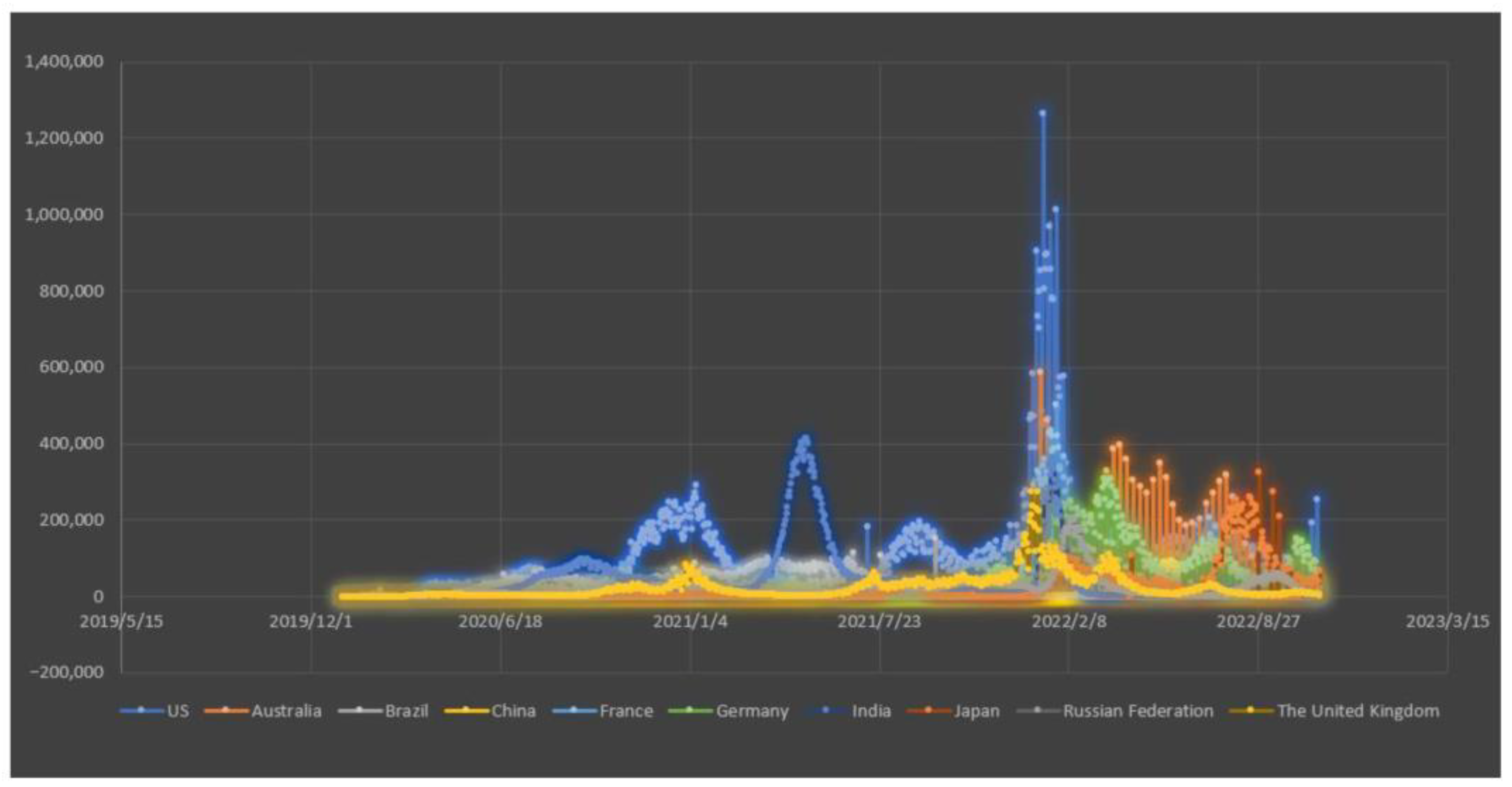
During almost the entire COVID-19 pandemic period, the Chinese government implemented a dynamic zeroing-out policy (The ‘dynamic zeroing-out’ policy is an epidemic prevention policy used to combat infectious diseases, particularly severe acute respiratory syndrome. When a confirmed case is identified, epidemiological investigations are carried out simultaneously with medical treatment measures. All persons who may have come into contact with the virus are quarantined, and the spread of the virus is controlled in order to reduce the number of cases. In response to the outbreak of the COVID-19 pandemic in early 2019, mainland China, as well as Australia, New Zealand, and other regions, adopted this policy to prevent the collapse of their healthcare system and reduce the number of severe cases and deaths.) (Up until the end of 2022, the Chinese government began to shift its dynamic zeroing-out policy to the precise prevention and control policy, following which, the number of daily new-added COVID-19 confirmed cases increased rapidly, with medical protective equipment and drugs for treating COVID-19, such as masks and antipyretics, being out of stock.) to contain the spread of COVID-19 [3], which was highly effective in suppressing the spread of the virus, as shown in Figure 1. From the end of 2019 to the end of 2022, the daily increase in COVID-19 confirmed cases in China was significantly lower than those of other major countries in the world, which was indeed attributed to China’s strict implementation of the dynamic zeroing-out policy.
With the emergence and spread of COVID-19 and its impact on all sectors of society, relevant research has been carried out gradually. Currently, the basic reproduction number R0 [4] is used to signify the transmissibility of a virus (the basic reproduction number (R0) is the number of cases directly caused by an infected individual throughout his infectious period. R0 is used to determine the ability of a disease to spread within a given population. The reproduction number (R0) represents the transmissibility of a disease.) in the Science of Public Health, and the changes in R0 are supposed to reflect the situation of virus mutations and the effectiveness of governmental virus-containment policies. Therefore, R0 is thought to be an important indicator for governments to adjust virus-containment policies in a pandemic setting, and it is crucial to measure the value of R0 in time and in an accurate way. However, during the COVID-19 pandemic, more attention was paid to the daily increase in confirmed cases rather than the changes in R0 due to the difficulties that come with its measurement. In another word, the traditional method used to estimate R0 can only obtain a constant value in a certain period of time. However, as a matter of fact, R0 for COVID-19 varied over time and places, and it is not a constant value but a time-varying sequence.
So far, there are few methods that have been used to quantify the virus transmission rate that are related to a time-varying sequence on daily data of an outbreak in affected areas, meaning that the changes in COVID-19 transmission rate, as well as the effectiveness of governmental measures for containing the spread of COVID-19, are hard to reflect in a timely and dynamic manner. Hence, this paper aims to fill this gap by constructing a model that can help to estimate the dynamic COVID-19 transmission rate. To achieve this, we used a rolling time series to construct a model and calculated the COVID-19 transmission rate in mainland China.
Additionally, to verify the validity of this measurement method, after estimating the dynamic COVID-19 transmission rate, the daily returns of stock markets in China were used as explained variables to explore the impact of the COVID-19 transmission rate on stock markets, and the results revealed that the COVID-19 transmission rate had a significantly negative impact on stock markets, which, to some extent, confirms the validity of this method and provides evidence that proves the long-term impact of the COVID-19 pandemic on stock markets.
These things considered, this paper chose mainland China as a research sample based on the following two reasons: First, mainland China implemented a dynamic zeroing-out policy to contain COVID-19, which resulted in a rather long period when the daily increase in COVID-19 confirmed cases remained below 10, inhibiting the use of the traditional methods of estimating virus transmission rates to obtain the specific value of R0 that could reflect the true epidemic situation in mainland China. Second, due to the dynamic zeroing-out policy, the data regarding daily increases in confirmed cases of COVID-19 in mainland China were relatively accurate, which ensured that, when using these data to estimate COVID-19 transmission rate, there would be no need to worry about missed, delayed, mistaken, or false reports.
Moreover, the method developed in this paper is not only applicable to the COVID-19 pandemic but also to other global or regional epidemics that have occurred or may occur, and it is also applicable to determine the dynamic transmission rate of other pathogens, including but not limited to viruses spreading among human beings. At the same time, the findings of this paper can also provide some insights that could inform the anti-epidemic work of governments, for instance, regulating the intensity of anti-epidemic measures to keep a better balance between virus-containing efforts, the free movement of the population, and economic development. Last but not least, it can also provide a reference for investors and stakeholders to make decisions when they need to change their business strategies in pandemic settings.
This paper consists of three main parts, namely, Method for the Measurement of COVID-19 Transmission Rate, COVID-19 Transmission Rate and its Impact on Stock Markets, and conclusions and prospects. First, the rolling time series model was employed and used to estimate the COVID-19 transmission rate in mainland China. Second, the obtained values for the COVID-19 transmission rate were used as explanatory variables and China’s stock indices as explained variables for regression analysis to investigate the impact of the COVID-19 transmission rate on China’s stock markets, and the obtained results showed a significant negative correlation between the COVID-19 transmission rate and China’s stock indices. Finally, further discussions and analyses were made regarding the above content, and relevant opinions were given to policymakers and stock investors.
1.2. Literature Review
1.2.1. Definition and Calculation of Basic Reproductive Number R0
In epidemiology, the basic reproduction number, denoted with R0, is used to define the transmission rate of a virus. However, R0 is a theoretical value with limited practical utility in the real word. On the other hand, R0, referred to as the basic reproductive number, is a fundamental metric used to measure the potential spread of a virus. It specifically represents the expected number of secondary infected cases that result from a single infected one in a population where all individuals are susceptible to infection.
This metric is an important predictor of disease transmission dynamics and serves as a critical tool for informing public health policies aimed at controlling disease outbreaks [5,6], with the presupposition that there will be no infection or immunization among individuals, whether acquired or through vaccination. Some other definitions, such as the one put forth by the Australian Department of Health, also incorporate the requirement that there be no deliberate interference with disease transmission [7].
Siegel E believed R0 is a dimensionless quantity that represents the number of individuals who might be infected by an infected one, which should not be confused with time rate. The time rate has units of time−1 such as doubling time. This kind of distinction is important when considering the spread and control of infectious diseases [8].
Various methods have been developed to calculate R0, such as the survival function, the manipulation of the dominant eigenvalue of the Jacobian matrix, the next-generation method [9], the evaluation of intrinsic growth rate [10], the analysis of endemic equilibrium, the estimation of the number of susceptible individuals at the endemic equilibrium, the determination of the average age of infection [11], and the final size equation [12]. However, Li, Blakeley, and Smith supposed that there be little consensus among these methods, with significant disagreement even when analyzing the same system of differential equations [13]. Furthermore, Heffernan, Smith, and Wahl believed that only a small subset of these methods were capable of calculating the average number of secondary infections. The particular problem is that R0 can seldom be directly observed in real-world settings and must be estimated through a mathematical model instead, which thereby reduces its practical applicability [14].
The value of R0 is solely determined by the characteristics of the virus itself and does not change with any external environmental factors [15]. For example, the R0 value of COVID-19 (Alpha variant) is 4–5 [16]; the R0 value of COVID-19 (ancestral strain) is 2.9 (2.4−3.4) [16]; the R0 value of COVID-19 (Delta variant) is 5.1 [17]; and the R0 value of COVID-19 (Omicron variant) is 9.5 [18]. In order to let R0 reflect the transmission rate in the real world, this paper uses a time series method to measure the dynamic COVID-19 transmission rate to calculate the actual dynamic R0 so as to reflect the dynamic COVID-19 transmission rate in the real world.
1.2.2. Measurement of COVID-19 Transmission Rate
Nowadays, there is also a growing focus on COVID-19 transmission rate in the real world as it is an important indicator used to characterize a virus capable of causing an epidemic. Johnson et al. investigated whether public green spaces would decrease COVID-19 transmission rate by building a baseline transmission model and using variables, i.e., the changes in mobility, baseline health, and population density, to explore the effect of green spaces on COVID-19 transmission rate [19], while Carleton and Meng employed a relatively simple method to study the effect of temperature on the COVID-19 transmission rate by establishing a model in which the logarithm of the daily increased number of COVID-19 confirmed cases was used as an explained variable [20]. Furthermore, Mahmoudi et al. compared different COVID-19 transmission rates in high-risk countries such as the United States, Germany, the United Kingdom, and Italy via a fuzzy clustering method using artificial intelligence [21]. However, the COVID-19 transmission rate was not specifically calculated in these studies.
Samui, Mondal, and Khajanchi developed the SAIU (susceptible or uninfected-asymptomatic-reported symptomatic infectious-unreported symptomatic infectious) model system to analyze the COVID-19 transmission rate in India and accurately predicted the transmission process of COVID-19 in India for the next 60 days [22]. In their study, the researchers noted that the COVID-19 transmission rate in India was not a constant value but a dynamic sequence that was changing over time, which provided a foundation for subsequent research by Mbuvha and Marwala [23].
Mbuvha and Marwala conducted an analysis of the COVID-19 transmission rate in South Africa using the SEIR (susceptible-exposed-infectious-recovered) and SIR (classical susceptible-infectious-removed) models and proposed that the COVID-19 transmission rate was not constant but a time-varying sequence [24]. Subsequently, they used MCMC and publicly available data to perform Bayesian parameter inference on the SIR and SEIR model. The estimated results of the parameters were consistent with the mean baseline R0 prior to governmental intervention, the mean latency, and the mean infection in the existing literature.
The existing literature relevant to this study mainly focused on predicting the increase in confirmed COVID-19 cases in the days that followed without demonstrating methods to calculate the COVID-19 transmission rate based on the daily increase in confirmed COVID-19 cases. As a matter of fact, in characterizing a virus that capable of causing an epidemic, the transmission rate is superior to the number of daily increases in confirmed cases because the daily increased number of confirmed cases is influenced by that of the previous day, with which the immediate epidemic situation cannot be reflected in an apparent way due to scholars and researchers having to take their time and wait for accumulated effects. Instead, the transmission rate can solve this problem. Take China for an example, the government implemented lockdown measures on 23 January 2020, but the daily increase in COVID-19 confirmed cases lasted until almost 10 days after lockdown. This means that the number of daily increases in confirmed cases had a lag response to the anti-epidemic policies, which is the weakness of using the number of confirmed cases to measure an epidemic. Therefore, we managed to solve this problem by calculating the COVID-19 transmission rate based on the time series method to avoid that kind of lag effect (Suppose that at time ta, the number of daily increase in confirmed cases is 50, and at ta+1 it is 100; while at time tb the number of daily increase in confirmed cases is 500, and at tb+1 it is 550. The difference in the number of the increase in confirmed cases between time ta and tb is 50, but the ability of infected people to transmit the virus at time tb is significantly lower than at time ta.).
1.2.3. Impact of COVID-19 on Stock Markets
Currently, many researchers have analyzed the impact of COVID-19 on stock markets. Al-Awadhi et al. conducted an empirical analysis on the Hang Seng Index and the Shanghai Composite Index, concluding that the number of confirmed cases and deaths from COVID-19 have had a negative impact on China’s stock markets [25,26]. Ashraf further analyzed the impact of daily increases in confirmed COVID-19 cases and deaths on stock markets with data obtained from 64 countries. He established an OLS model for analysis and revealed that the negative impact of the increases in confirmed COVID-19 cases on stock markets was greater than that of deaths and that the COVID-19 pandemic had the greatest impact on stock markets between the 40th and 60th days after COVID-19 broke out [27]. Phan and Narayan carried out further research based on Ashraf’s study using descriptive statistics. They observed the performance of stock markets in 25 countries after the pandemic occurred and found that, when the number of COVID-19 confirmed cases reached 100,000 or the number of deaths reached 100 in a country, 50% of stocks would rise due to potential correction effects caused by the impact of the pandemic on markets [28].
The current mainstream beliefs in the academic field state that the COVID-19 pandemic only had short-term effects on stock markets. However, Xe et al. found a long-term and significant causal relationship between the Shanghai Composite Index and the number of confirmed cases and deaths from COVID-19 [29]. Huang and Liu found that the impact of the COVID-19 pandemic on the stock prices of China’s energy companies still existed within three months after its outbreak, indicating a mid- and long-term impact on stock markets [30]. Yousfi et al. provided some new evidence for such an impact, and they found that the first and second waves of COVID-19 in the United States enhanced stock-market uncertainty and that the second wave had a greater impact than the first [31].
Therefore, this paper believes that COVID-19 pandemic objectively has a long-term impact on stock markets. However, using the daily increase in confirmed cases or deaths of COVID-19 as an explanatory variable is hard to reveal such a long-term impact on stock markets. Therefore, this paper attempts to use COVID-19 transmission rate as an explanatory variable to study the long-term impact of COVID-19 on China’s stock markets.
2. Method for Measurement of COVID-19 Transmission Rate
2.1. Definition of COVID-19 Transmission Rate
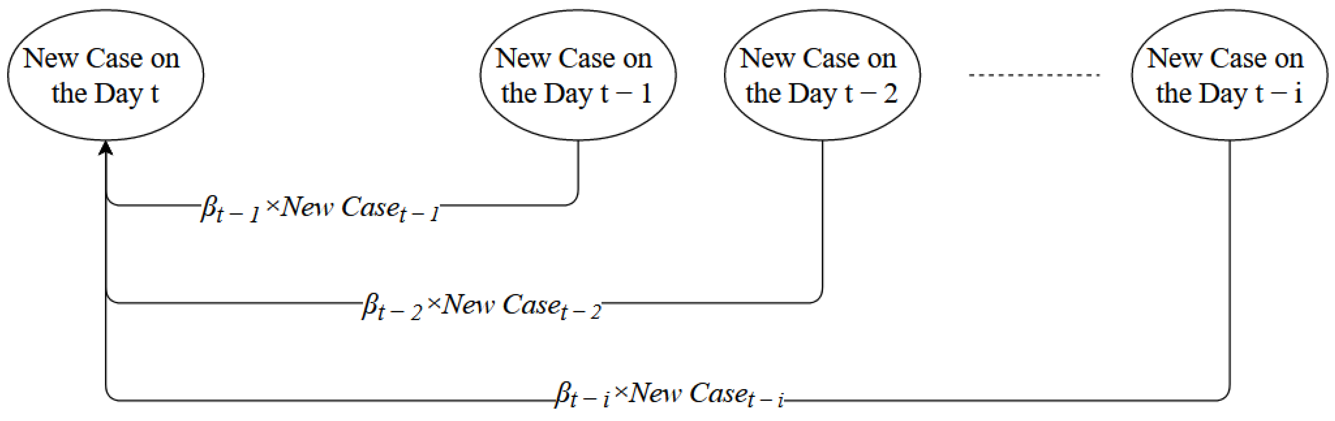
COVID-19 is mainly transmitted from person to person [30]. The number of newly added confirmed COVID-19 cases on Day t is regarded as the patients who were infected with COVID-19 during the days from Day t − 1 to Day t − i, and they transmitted the virus to the people who were tested positive on Day t. This process is shown in Figure 2. Following Figure 2, let the number of COVID-19 confirmed cases on Day t be New Cases, and then let the COVID-19 transmission rate on Day t − i be βt−i.
Then, Equation (1) is written as follows:
βt−i is a 1 × i column vector, and New Caset−i is a i × 1 row vector. New Caset−i represents the number of newly added confirmed COVID-19 cases on Day t − i, and βt−i × New Caset−i represents the number of newly added confirmed COVID-19 cases during the days from Day t − 1 to Day t − i who were infected and tested positive on Day t. The value of i represents the time window during which someone infected with COVID-19 is capable of transmitting the virus, and those infected are considered to lose the ability to transmit the virus when they recover or are quarantined from others.
For this paper, data covering the days from 19 January 2020 to 28 October 2022 in mainland China (excluding Hong Kong, Macau, and Taiwan) were selected. All of the data were obtained from the database of the National Health Commission of the People’s Republic of China (Data source: http://www.nhc.gov.cn/, accessed on 28 October 2022)
The reason for choosing mainland China as the research object is because mainland China implemented a dynamic zeroing-out policy during the COVID-19 pandemic. According to the dynamic zeroing-out policy in mainland China, positive COVID-19 cases would be immediately isolated from the others just after testing positive for infection, that is, the time of free movement for COVID-19 patients in mainland China should not exceed 1 day, so set i = 1. Then, Equation (2) can be obtained as follows:
Due to the fact that COVID-19 testing is not 100% accurate, false positives and negatives have to be taken into consideration. Therefore, εt(2) is used to represent the number of false positive or negative cases. According to information released on the official website of the Yunnan Provincial People’s Government (Information source: https://www.yn.gov.cn/, accessed on 16 May 2023), the accuracy of COVID-19 testing was more than 95%, but there were still cases of false positives or negatives. False positives were counted as newly added cases every day, while false negative cases were considered to possess a high probability of transmitting the disease to others for more than 24 h.
2.2. Measurement of COVID-19 Transmission Rate
As a matter of fact, the daily newly added confirmed COVID-19 cases in mainland China had been in single digits for quite a long period during the COVID-19 pandemic due to the dynamic zeroing-out policy implemented by the government. Here, in order to check the above calculation method, take a certain COVID-19 period in mainland China as an example, i.e., on Day tk−1, mainland China had one newly added confirmed COVID-19 case; on Day tk, mainland China had five newly added confirmed COVID-19 cases; on Day tk+1, mainland China had nine newly added confirmed COVID-19 cases; and on Day tk+2, mainland China had five newly added confirmed COVID-19 cases. Then, based on the equation βt−1 = (New Caset − εt(2))/New Caset−1, the calculated results are shown as βt(k−1) = 500%, βt(k) = 180%, and βt(k+1) = 0.55%. It can be seen that these four days all involve the changes of only four cases, but the value of βt−1 obtained through the equation of βt−1 = (New Caset−εt(2))/New Caset−1 drastically fluctuates. Therefore, using this method to estimate the COVID-19 transmission rate in mainland China is not suitable.
In order to ensure that the value of βt−1 does not fluctuate too much and that it reflects the COVID-19 transmission rate in mainland China more objectively and accurately, this paper selected a time series method.
Equation (2) is similar in form to an Auto-regressive Model, but unlike an AR(1) model, where the value of α1 in xt = α1xt−1 + εtn is constant, the value of βt−1 in Equation (2) is a time-varying sequence. In order to obtain the time-varying sequence of βt−1, this paper selected an AR(1) model and employed a rolling time series to estimate βt−1.
When estimating the COVID-19 transmission rate using a rolling time series, the prerequisite is that the COVID-19 transmission rate is constant within the selected time window, and theoretically, the shorter the selected time window, the closer the estimated result approaches the true value. Furthermore, based on the central limit theorem, when a certain condition is met for a random variable, its sample mean would follow a normal distribution, and when the sample size is greater than 30, the normal distribution would better approximate the sample mean distribution [32,33]. This paper selected the duration of 30 days, 40 days, 50 days, and 60 days as the time windows to estimate the COVID-19 transmission rate, as is shown in Figure 3. The results with a time window of 30 days are of a stable fluctuation, with main data fluctuating around 1, without outliers, which is consistent with the actual situation of COVID-19 transmission in mainland China. Therefore, a time window of 30 days was chosen for this paper.
Concretely, a rolling time series model was used to calculate the COVID-19 transmission rate in mainland China. By taking 30 days as the time window to obtain the data of daily newly added confirmed COVID-19 cases between 19 January 2020 and 18 February 2020 and inserting these data into Equation (2), the corresponding value of βt−1 is obtained, which is considered as the COVID-19 transmission rate in mainland China on 19 January 2020. Using the same method to obtain the data of daily newly added confirmed COVID-19 cases between 20 January 2020 and 19 February 2020, and inserting the data into Equation (2), the corresponding βt−1 value is obtained, which is considered as the COVID-19 transmission rate in mainland China on 20 January 2020. If βt−1 is greater than 1, it can be considered that COVID-19 is spreading in mainland China; if βt−1 is smaller than 1 but greater than 0, it can be considered that COVID-19 is effectively contained in mainland China.
2.3. Processing Methods and Explanations for Non-Stationary Time Series
This paper utilized the data involving daily newly added confirmed COVID-19 cases between 19 January 2020 and 28 October 2022, including 985 observations in total. ADF(Augmented Dickey–Fuller) test was conducted on each of them, and some of the results exhibited unit roots while others did not. After applying first-order difference, all the time series that previously exhibited unit roots passed the ADF test, and then none had unit roots.
For the series with the unit root, the model is modified to Equation (3).
Rearrange Equation (3) to Equation (4).
In Equation (4), (β* + 1) represents the COVID-19 transmission rate of Day t − 1 on Day t, while −β* represents the COVID-19 transmission rate of Day t − 2 on Day t. If β* < 0, then −β* > 0, suggesting that on Day t, the number of daily newly added confirmed COVID-19 cases from both Day t − 1 and Day t − 2 have the ability to transmit the virus, indicating a weakening detection and a risk of potential outbreak during this period, but not necessarily guaranteeing that an outbreak will occur. However, if β* > 0, it signifies a more complex situation that requires further analysis.
Rearrange Equation (4) to Equation (5),
When New Caset−1 > New Caset−2 and β* > 0, it can be inferred that the virus is in the outbreak phase. Specifically, on Day t, the number of newly added confirmed COVID-19 cases increases by β* × (New Caset−1-New Caset−2) on the base of the number of newly added confirmed COVID-19 cases on Day t − 1. Conversely, when New Caset−1 < New Caset−2, the virus is deemed to be under control, indicating that, on Day t, the number of newly added confirmed COVID-19 cases decreases by β* × (New Caset−1 − New Caset−2) on the base of the number of newly added confirmed COVID-19 cases on Day t − 1.
To recap, there are three coefficients of COVID-19 transmission rate: βt−1, (β* + 1), and β*. The former two indicate the transmission rate on Day t − 1, while the latter indicates the transmission rate on Day t − 2.
2.4. Determination of p in AR(p) and Diagnosis of Residuals
This paper chose an AR(1) model for regression. Based on the value of AIC and BIC, an AR(1) model was considered most applicable to the situation of mainland China. Then, we conducted the White Noise Test on the residuals of each time series to check whether the model employed in this paper was correct or not, and the results indicated that the residuals passed the test. This suggested that they were independent and identically distributed. In Section 2.1, we discussed that the residual is caused by the occurrence of false positive and negative cases in regard to COVID-19 testing. If false negative cases can cause widespread transmission, an ARMA model should be constructed. However, under the dynamic zeroing-out policy, the false negative cases do not have the opportunity for widespread transmission. Therefore, we believe that MA(q) does not need to be added to the model.
In addition, during the research period, the Chinese government implemented the dynamic zeroing-out policy. The policy requested residents to undergo COVID-19 testing every day to identify positive cases and those who needed to isolate at once. Residents without negative test results within the last 24 h were not allowed to enter any public places, such as schools, shops, hospitals, etc. For residents who tested positive, they were requested to go directly to designated hospitals for isolation and treatment. Daily newly added cases were reported every day by the testing departments of the National Health Commission of the People’s Republic of China. Therefore, there was a lower probability of missed, delayed, and false reporting, etc., ensuring the accuracy of the daily new-added data. Additionally, the Chinese government requested people from abroad (foreign countries, Hong Kong, Macao, Taiwan) to undergo 21 days of quarantine and take no less than three tests during the quarantine period to ensure that few cases were imported into mainland China. Based on this, AR(1) is suitable for the conditions of mainland China.
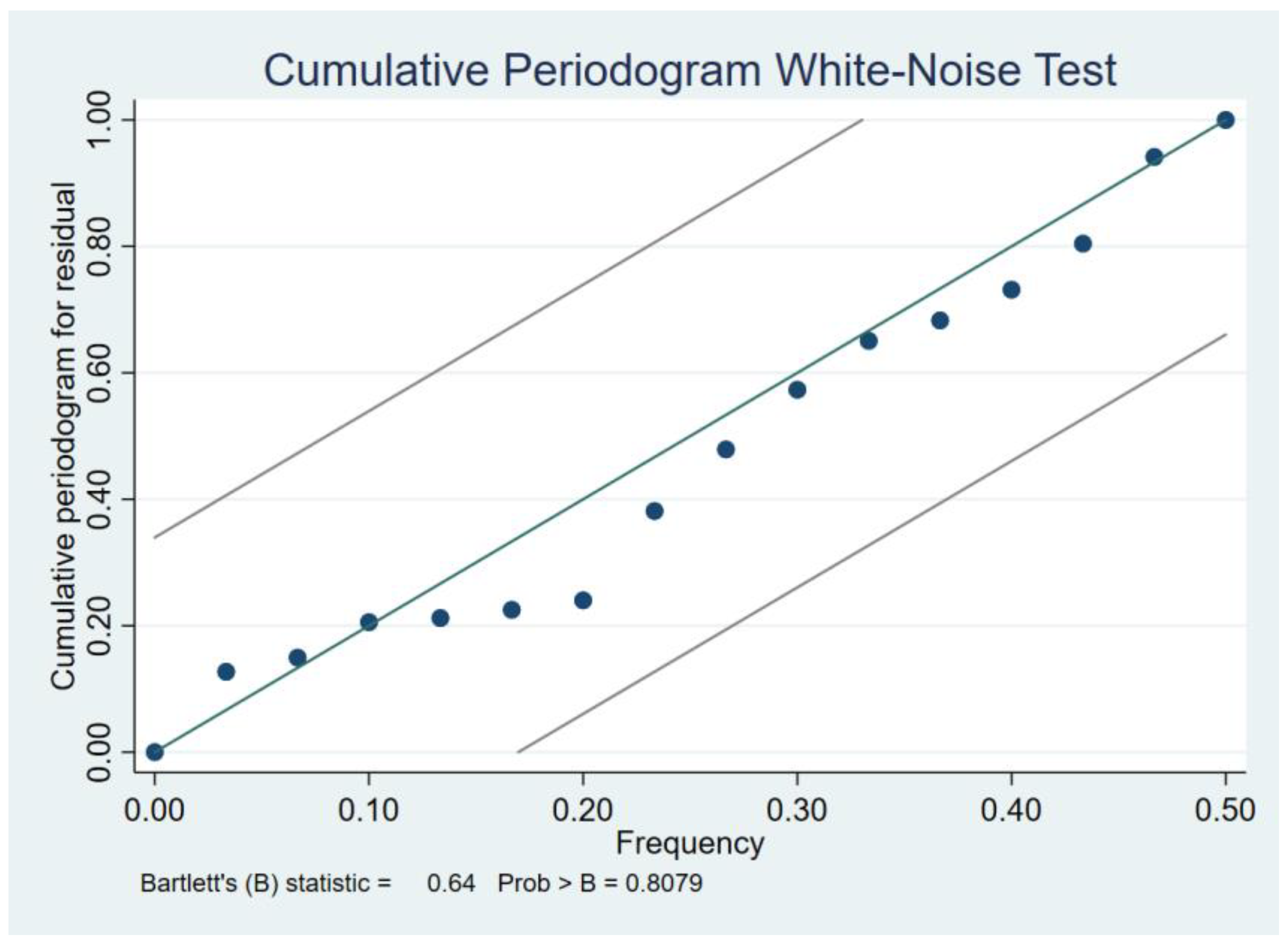
In order to test whether the residuals of AR(1) regressions were white noise or not, White Noise Tests were conducted on 985 time series, and the outcome of the first time window, which is displayed in Figure 4, showed that all points were within the detection line range and that the p-value for the test was 0.8079 (significantly greater than 0.05), which indicated that the residuals could be considered as white noise. Furthermore, the results of other time windows are consistent with the first time window, though they are not displayed one by one in the paper.
3. COVID-19 Transmission Rate and Its Impact on Stock Market
3.1. Estimated Results of COVID-19 Transmission Rate
The data regarding COVID-19 were obtained from the National Health Commission of the People’s Republic of China Database. The sample period ranged from 19 January 2020 to 28 October 2022, including 985 observations in total. The estimated results are shown in Figure 5.
Based on Section 2.3, the COVID-19 transmission rate of Day t − 1 is βt−1 or (β* + 1) and that of Day t − 2 is −β* or 0. The average of the COVID-19 transmission rate of Day t − 1 is 0.811, which is smaller than 1, indicating that COVID-19 in mainland China is under control. However, the maximum value of the COVID-19 transmission rate of Day t − 1 is 1.445, indicating that there is still a period of COVID-19 outbreak in mainland China.
As shown in Figure 5, the value of the COVID-19 transmission rate of the first day is basically below 1, while the value of the second day often accompanies a decrease in that of the first day, which indicates that the dynamic zeroing-out policy has effectively contained the spread of COVID-19 and eliminated potential COVID-19 outbreaks.
Figure 5 shows that it is apparent that, in the first half of COVID-19 pandemic, roughly until the middle of 2021, the fluctuations in the COVID-19 transmission rate in mainland China were relatively small compared with the latter half. Additionally, the data regarding the COVID-19 transmission rate of the first day were always smaller than 1, and those of the second day were mostly 0. This indicates that the spread of COVID-19 was effectively controlled during this period under the dynamic zeroing-out policy implemented by the Chinese government. After mid-2021, the COVID-19 transmission rate in mainland China fluctuated more intensely. The transmission rate of the first day was greater than 1, accompanied by that of the second day, which was greater than 0 at times, indicating that COVID-19 had broke out in parts of mainland China during those periods, which is mainly related to several factors. Firstly, the Chinese government attempted to alleviate the impact of COVID-19 on economic development by relaxing the COVID-19 containment policy. Secondly, the mutation of COVID-19 has made in-time detection more difficult. Lastly, the continued implementation of the zeroing-out policy was not so strict as it used to be.
3.2. Impact of COVID-19 Transmission Rate on China’s Stock Markets
To verify the accuracy and practicality of the method developed in this paper, the COVID-19 transmission rate estimated in previous sections was taken as the explanatory variable, and the daily returns of the Hang Seng China Enterprises Index (HSCEI), SSE Composite Index (SSE), and Shenzhen Component Index (SZSE) stock indices as explained variables to conduct an empirical analysis, exploring the long-term impact of the COVID-19 transmission rate on China’s stock markets.
3.2.1. Model Specification
This paper takes Hang Seng China Enterprises Index (HSCEI), SSE Composite Index (SSE), and Shenzhen Component Index (SZSE) as research objects. The return of the index is represented by Ri,t, and the logarithm of the index is represented by log(Indexi,t), both of which are utilized in constructing a panel data model, with the COVID-19 transmission rate serving as an explanatory variable and Ri,t as the explained variable.
Drawing on the works of Ashraf and Feng, GDP, CPI, and Long-term Policy Interest Rate are chosen as control variables [27,34]. To further capture the impact of RMB exchange rate and monetary policy on stock markets, M2 and CFETS RMB Exchange Rate Index are also included as control variables. Moreover, in order to mitigate the effects of the stock markets in the US and Singapore on China’s stock markets, the S&P 500 Index, NASDAQ Composite Index, and FTSE Singapore STI Index are added as control variables as well, and the log returns of stock indices for these control variables are also calculated. The definition of the variables is shown in Table 1.
ADF tests were conducted on the explained variables, explanatory variables, and control variables, and the results indicate that the null hypothesis is rejected at a 5% significance level. This suggests that there are no unit roots for any of the variables and that the conditions for co-integration tests have been met.
A co-integration test was conducted to determine whether there exists a long-term equilibrium relationship among the endogenous variables in the model. The Kao ADF method was employed for this purpose, and the results indicate that the null hypothesis is rejected at a 5% significance level, signifying the presence of a co-integration relationship among the variables, thus enabling regression analysis to be performed on them.
After conducting the F-test, it was found that there existed an individual fixed effect but no time fixed effects. Therefore, an individual fixed effect model was established and the model is shown in Equation (7).
The COVID-19 transmission rate, denoted by xit, is represented as a 2 × 1 vector, comprising the transmission rate on the first day and second day, which were obtained in Section 2.3. Meanwhile, δit represents control variables and is an 8 × 1 vector. μi represents the individual fixed difference that does not change over time, cit is the constant, and εit is residual.
3.2.2. Data Sources and Descriptive Statistics
Hang Seng China Enterprises Index (HSCEI), SSE Composite Index (SSE), and Shenzhen Component Index (SZSE) were sourced from the Wind database. The COVID-19 transmission rate was used as the explanatory variable, and the data were obtained from the National Health Commission of the People’s Republic of China Database. The sample period ranged from 19 January 2020 to 28 October 2022. Control variables included NASDAQ Composite Index (IXIC.GI), S&P 500 Index (SPX.GI), FTSE Singapore STI Index (STI.GI), long-term policy interest rate of the People’s Bank of China, CFETS RMB exchange rate index, CPI of China, real GDP of China, and M2 of China, with all data obtained from the Wind database.
Since the data frequencies of the explained variable, explanatory variables, and control variables are inconsistent, this paper converted all these variables into 7-day weekly data. Eviews 12 was used to convert quarterly and monthly data. For missing stock index data, the data from the previous day were used. In other words, if the data for log(indext+1,i) were missing, then log(indext+1,i) would be set equal to log(indext,i).
Table 2 shows descriptive statistics, which display statistical features of the data involved in the model.
It can be seen in Table 2 that the mean of the first-day COVID-19 transmission rate is 0.811 (smaller than 1), which indicates that the dynamic zeroing-out policy effectively contained the overall spread of COVID-19. However, the maximum value is 1.45 (significantly greater than 1), which suggests that, even under the dynamic zeroing-out policy, there were still some brief outbreaks of COVID-19. The average (0.128) and the maximum (0.792) value of the second-day COVID-19 transmission rate are both significantly smaller than 1, and the median (p50) is 0, which indicates that, although the dynamic zeroing-out policy could not completely contain the spread of COVID-19, it still had strong error-correction capabilities and could ensure that the epidemic did not grow in scope to a large-scale, long-term one.
Table 2 also shows that the daily returns of HSCEI, SSZ, and SZSE are relatively stable from 19 January 2020 to 28 October 2022. Their mean returns are all close to 0, indicating that the three indices are relatively stable during the selected sample period. However, the returns of all three indices have a minimum value between −1.86% and −3.49% and a maximum value between 2.41% and 5.12%, indicating that the returns of the three indices are stable in the long term but that there are fluctuations in the short term.
3.2.3. Estimation Results
This paper selected an OLS model, mixed regression model, and fixed effect model to investigate the effect of the COVID-19 transmission rate on stock market indices in China, and the obtained results are shown in Table 3.
The results show a correlation between the COVID-19 transmission rate and stock market volatility. Concretely speaking, there was a negative impact of COVID-19 transmission rate on China’s stock markets. That is, the larger the COVID-19 transmission rate, the greater the negative impact on stock markets.
In detail, the regression coefficient for the first-day COVID-19 transmission rate is −0.00538, at 1% significance level. Numerically, for each-unit increase in the first-day COVID-19 transmission rate, i.e., a confirmed COVID-19 case infecting one healthy person to two healthy ones, the returns of the stock index decrease by 0.538%. Meanwhile, the regression coefficient for the second-day COVID-19 transmission rate is also negative, at 5% significance level, indicating that, during that outbreak period, the decline in the stock index was greater than 0.538%.
The COVID-19 transmission rate had an impact on China’s stock markets throughout the COVID-19 pandemic period, and the impact would last for a long period, which is inconsistent with the studies in the literature, which suggest that the impact of the COVID-19 pandemic on China’s stock markets was short-term.
3.2.4. Robustness Test
In order to further verify the relationship between the COVID-19 transmission rate and stock index return, using an OLS model, this paper conducted a regression for the daily return of HSCEI, SSZ, and SZSE, respectively. The results are shown in Table 4.
Based on the regression results in Table 4, the COVID-19 transmission rate negatively correlates with the daily returns of HSCEI. Numerically, for each-unit increase in the first-day COVID-19 transmission rate, i.e., a confirmed COVID-19 case infecting one healthy person to two healthy ones, the returns of HSCEI decrease by 0.797%. Meanwhile, the coefficient of the second-day COVID-19 transmission rate is also negative, indicating that, during the phase whereby COVID-19 rapidly spread, the returns of HSCEI decreased fast.
The one-period-lagged first-day COVID-19 transmission rate has a significant negative effect on the daily returns of SSE. Numerically, when the COVID-19 transmission rate increases by one unit, i.e., a confirmed COVID-19 case transmitting the virus from one healthy person to two healthy ones, the returns of SSE decrease by 0.390%.
The two-period-lagged first-day COVID-19 transmission rate has a significant negative effect on the daily returns of SZSE. Numerically, each-unit increase in the COVID-19 transmission rate, i.e., one confirmed COVID-19 case infecting one healthy person to two healthy ones, leads to a decrease of 0.648% in the returns of SZSE.
In conclusion, the empirical results suggest that the COVID-19 transmission rate has a negative impact on the returns of stock markets in China, and the result passed the robustness test. Moreover, the result of the robustness test indicates that the efficiencies of different stock markets vary from one another, with HSCEI being more sensitive to the changes in the COVID-19 transmission rate compared to SSE and SZSE. This implies that the Hong Kong stock market is closer to the efficient market than the other two markets in China. However, SSE and SESZ have a greater ability to withstand the impact of the changes in the COVID-19 transmission rate compared to HSCEI. In particular, SSE has a change of less than 0.5% in the returns corresponding to a unit change in the transmission rate of COVID-19, indicating that the Shanghai stock market has the strongest ability to resist uncertainty and risks.
4. Discussion and Prospects
This paper used the rolling time series to method construct a model to calculate the COVID-19 transmission rate, successfully obtained the COVID-19 transmission rate in mainland China, and then explored the impact of the COVID-19 transmission rate on China’s stock markets. Eventually, the results demonstrated that the change in the COVID-19 transmission rate had a significant and long-term impact on China’s stock indices; the increase in the COVID-19 transmission rate had a negative impact on China’s stock market, which is consistent with the existing literature.
In order to enable the model to be used in different countries or regions, some conditions should be taken into consideration. Firstly, to estimate the COVID-19 transmission rate using this method, the researchers need to identify the days when confirmed cases can move around freely in a specific country or region and then determine the value of p in an AR(p) model. The value of p depends on the specific situation of a country or region. Secondly, due to the dynamic zeroing-out policy implemented by the Chinese government, the accuracy of daily newly added confirmed COVID-19 cases can be ensured, while for most other countries, there are difficulties with collecting the data, namely, missed or delayed reporting, which may lead to inaccuracies in the number of daily newly added confirmed cases. Thirdly, based on the dynamic zeroing-out policy, China avoided the possibility of COVID-19 transmission from overseas, while, for countries, without implementing a strict testing and quarantine system, the levels of virus transmission from imported cases need to be considered. Therefore, using the ARMA (p, q) model may be more appropriate. Specifically, AR (p) represents the rate of COVID-19 transmission in the country, while MA (q) represents the rate of COVID-19 transmission from imported cases. Therefore, there are still many challenges in determining the values of p and q in the ARMA (p, q) model.
Although, in specific scenarios, this method requires solving certain data issues based on each country’s unique situation before estimating the COVID-19 transmission rate, the method provided in this paper still has universal applicability for estimating the COVID-19 transmission rate, as well as the transmission rate of other similar virus.
5. Conclusions
This paper used the rolling time series method to construct a COVID-19 transmission rate model, quantified the COVID-19 transmission rate in mainland China, and subsequently investigated the impact of COVID-19 transmission rate on the returns of HSCEI, SSE, and SESZ. The empirical results showed that the COVID-19 transmission rate had a negative impact on China’s stock markets, and this impact persisted throughout the pandemic period. The faster COVID-19 was transmitted, the greater the losses for stock market investors.
The response of different stock markets to changes in the COVID-19 transmission rate was also different. HSCEI had the fastest response, suggesting that the Hong Kong stock market was more timely in information processing than the other two stock markets of China and closer to the efficient market. SSE had the smallest variation in terms of returns, suggesting that the Shanghai stock market was more risk resistant than the other two markets.
In theory, using the model constructed in this paper, the dynamic transmission rate of a virus can be estimated. Additionally, in practice, there is a necessity to consider national situations and the features of the data related to the daily increase in confirmed cases when determining the period during which the infected individuals can freely spread the virus.
In this paper, mainland China was chosen as the research object because its efficiently implemented dynamic zeroing-out policy, which simplified the process of estimating the COVID-19 transmission rate. Therefore, we hope that future researchers would optimize the model for use in different countries or regions. At the same time, the method developed in this paper could also provide insights for governments to regulate and adjust anti-epidemic policies in a similar outbreak in the future, and the results may help investors to make decisions.
Author Contributions
H.X.: Conceptualization, methodology, software, formal analysis, writing—original draft preparation; D.L.: Writing—review, methodology, supervision; S.L.: Data curation and validation. All authors have read and agreed to the published version of the manuscript.
Funding
This research received no external funding.
Data Availability Statement
The data presented in this study are available upon request.
Acknowledgments
The authors wish to express their sincere thanks to the City University of Macau for its support and assistance in this study.
Conflicts of Interest
The authors declare no conflict of interest.
References
- Sohrabi, C.; Alsafi, Z.; O’Neill, N.; Khan, M.; Kerwan, A.; Al-Jabir, A.; Iosifidis, C.; Agha, R. World Health Organization declares global emergency: A review of the 2019 novel coronavirus (COVID-19). Int. J. Surg. 2020, 76, 71–76. [Google Scholar] [CrossRef] [PubMed]
- Yi, H.; Li, C.; Wang, P.; Cui, Z.; Xia, J.; Dai, S.; Liang, X. Global strategies for early prevention and control of the COVID-19 pneumonia outbreak. Chin. J. Prev. Med. 2020, 32, 325–329. Available online: https://kns.cnki.net/kcms2/article/abstract?v=3uoqIhG8C44YLTlOAiTRKibYlV5Vjs7i8oRR1PAr7RxjuAJk4dHXopF7w6tXxpKcEdsZdJXatnJHav6Cu5NT6GQVq_tBYwXI&uniplatform=NZKPT (accessed on 19 April 2023).
- Yang, Y.; Peng, F.; Wang, R.; Guan, K.; Jiang, T.; Xu, G.; Sun, J.; Chang, C. The deadly coronaviruses: The 2003 SARS pandemic and the 2020 novel coronavirus epidemic in China. J. Autoimmun. 2020, 109, 102434. [Google Scholar] [CrossRef] [PubMed]
- Dharmaratne, S.; Sudaraka, S.; Abeyagunawardena, I.; Katulanda, P.; Kariyawasam, J. Estimation of the basic reproduction number (R0) for the novel coronavirus disease in Sri Lanka. Virol. J. 2020, 17, 144. [Google Scholar] [CrossRef] [PubMed]
- Milligan, G.N.; Barrett, A.D. Chichester Vaccinology: An Essential Guide; Wiley Blackwell: West Sussex, UK, 2015; p. 310. [Google Scholar]
- Fraser, C.; Donnelly, C.A.; Cauchemez, S.; Hanage, W.P.; Van Kerkhove, M.D.; Hollingsworth, T.D.; Griffin, J.; Baggaley, R.F.; Jenkins, H.E.; Lyons, E.J.; et al. Pandemic potential of a strain of influenza A (H1N1): Early findings. Science 2009, 324, 1557–1561. [Google Scholar] [CrossRef]
- Becker, N.G.; Glass, K.; Barnes, B.; Caley, P.; Philp, D.; McCaw, J.M.; McVernon, J.; Wood, J. The reproduction number. In Using Mathematical Models to Assess Responses to an Outbreak of an Emerged Viral Respiratory Disease; National Centre for Epidemiology and Population Health: Acton, Australia, 2020; ISBN 1-74186-357-0. [Google Scholar]
- Siegel, E. Why ‘Exponential Growth’ Is So Scary For The COVID-19 Coronavirus. 2020. Available online: https://www.forbes.com/sites/startswithabang/2020/03/17/why-exponential-growth-is-so-scary-for-the-covid-19-coronavirus/ (accessed on 27 April 2023).
- Jones, J.H. Notes on R0; Stanford University: Stanford, CA, USA, 2007. [Google Scholar]
- Chowell, G.; Hengartner, N.W.; Castillo-Chavez, C.; Fenimore, P.W.; Hyman, J.M. The basic reproductive number of Ebola and the effects of public health measures: The cases of Congo and Uganda. J. Theor. Biol. 2004, 229, 119–126. [Google Scholar] [CrossRef]
- Ajelli, M.; Iannelli, M.; Manfredi, P.; Ciofidegli Atti, M.L. Basic mathematical models for the temporal dynamics of HAV in medium-endemicity Italian areas. Vaccine 2007, 26, 1697–1707. [Google Scholar] [CrossRef]
- Csefalvay, C. Simple compartmental models: The bedrock of mathematical epidemiology. In Computational Modeling of Infectious Disease; Academic Press: Cambridge, MA, USA, 2023; pp. 19–91. ISBN 9780323953894. [Google Scholar] [CrossRef]
- Li, J.; Blakeley, D.; Smith, R.J. The failure of R0. Comput. Math. Methods Med. 2011, 2021, 527610. [Google Scholar] [CrossRef]
- Heffernan, J.M.; Smith, R.J.; Wahl, L.M. Perspectives on the basic reproductive ratio. J. R. Soc. 2005, 2, 281–293. [Google Scholar] [CrossRef]
- Prather, K.A.; Marr, L.C.; Schooley, R.T.; McDiarmid, M.A.; Wilson, M.E.; Milton, D.K. Airborne transmission of SARS-CoV-2. Science 2020, 370, 303–304. [Google Scholar] [CrossRef]
- James, G. Covid: Is There a Limit to How Much Worse Variants Can Get? BBC News, 12 June 2021.
- Billah, A.; Miah, M.; Khan, N. Reproductive number of coronavirus: A systematic review and meta-analysis based on global level evidence. PLoS ONE 2020, 15, e0242128. [Google Scholar] [CrossRef]
- Liu, Y.; Rocklöv, J. The reproductive number of the Delta variant of SARS-CoV-2 is far higher compared to the ancestral SARS-CoV-2 virus. J. Travel Med. 2021, 28, taab124. [Google Scholar] [CrossRef] [PubMed]
- Johnson, T.F.; Hordley, L.A.; Greenwell, M.P.; Evans, L.C. Associations between COVID-19 transmission rates, park use, and landscape structure. Sci. Total Environ. 2021, 789, 148123. [Google Scholar] [CrossRef]
- Carleton, T.; Meng, K.C. Causal empirical estimates suggest COVID-19 transmission rates are highly seasonal. MedRxiv, 2020. [Google Scholar] [CrossRef]
- Mahmoudi, M.R.; Baleanu, D.; Mansor, Z.; Tuan, B.A.; Pho, K.H. Fuzzy clustering method to compare the spread rate of COVID-19 in the high risks countries. Chaos Solitons Fractals 2020, 140, 110230. [Google Scholar] [CrossRef] [PubMed]
- Samui, P.; Mondal, J.; Khajanchi, S. A mathematical model for COVID-19 transmission dynamics with a case study of India. Chaos Solitons Fractals 2020, 140, 110173. [Google Scholar] [CrossRef] [PubMed]
- Mbuvha, R.; Marwala, T. Bayesian inference of COVID-19 spreading rates in South Africa. PLoS ONE 2020, 15, e0237126. [Google Scholar] [CrossRef] [PubMed]
- Liu, Y. The effective reproductive number of the Omicron variant of SARS-CoV-2 is several times relative to Delta. J. Travel Med. 2022, 29, taac037. [Google Scholar] [CrossRef]
- Al-Awadhi, A.M.; Alsaifi, K.; Alhammadi, S. Death and contagious infectious diseases: Impact of the COVID-19 virus on stock market returns. J. Behav. Exp. Financ. 2020, 27, 100326. [Google Scholar] [CrossRef]
- Álvarez Aldeán, J.; Aristegui, J.; López-Belmonte, J.L.; Pedrós, M.; Sicilia, J.G. Economic and psychosocial impact of rotavirus infection in Spain: A literature review. Vaccine 2014, 32, 3740–3751. [Google Scholar] [CrossRef]
- Ashraf, B.N. Stock markets’ reaction to COVID-19: Cases or fatalities? Res. Int. Bus. Financ. 2020, 54, 101249. [Google Scholar] [CrossRef]
- Phan, D.H.B.; Narayan, P.K. Country responses and the reaction of the stock market to COVID-19—A preliminary exposition. Emerg. Mark. Financ. Trade 2020, 56, 2138–2150. [Google Scholar] [CrossRef]
- Xu, Y.; Zhao, Y.; Liu, M.; Xie, C. Research on risk contagion among financial submarkets in China based on complex networks. Entropy 2022, 24, 1120. [Google Scholar] [CrossRef] [PubMed]
- Huang, S.; Liu, H. Impact of COVID-19 on stock price crash risk: Evidence from Chinese energy firms. Energy Econ. 2021, 101, 105431. [Google Scholar] [CrossRef]
- Yousfi, M.; Zaied, Y.B.; Cheikh, N.B.; Lahouel, B.B.; Bouzgarrou, H. Effects of the COVID-19 pandemic on the US stock market and uncertainty: A comparative assessment between the first and second waves. Technol. Forecast. Soc. Chang. 2021, 167, 120710. [Google Scholar] [CrossRef] [PubMed]
- Fischer, H. A History of the Central Limit Theorem: From Classical to Modern Probability Theory; Springer: New York, NY, USA, 2011; pp. 1–10. [Google Scholar]
- Montgomery, D.C.; Runger, G.C. Applied Statistics and Probability for Engineers, 6th ed.; John Wiley & Sons: Hoboken, NJ, USA, 2014; p. 241. [Google Scholar]
- Feng, G.F.; Yang, H.C.; Gong, Q.; Chang, C.P. What is the exchange rate volatility response to COVID-19 and government interventions? Econ. Anal. Policy 2021, 69, 705–719. [Google Scholar] [CrossRef]
Figure 1.
Daily new confirmed cases of COVID-19 in different countries. Data are sourced from the World Health Organization official website. https://covid19.who.int/ (accessed on 31 October 2022).
Figure 1.
Daily new confirmed cases of COVID-19 in different countries. Data are sourced from the World Health Organization official website. https://covid19.who.int/ (accessed on 31 October 2022).

Figure 2.
Process of COVID-19 Transmission.

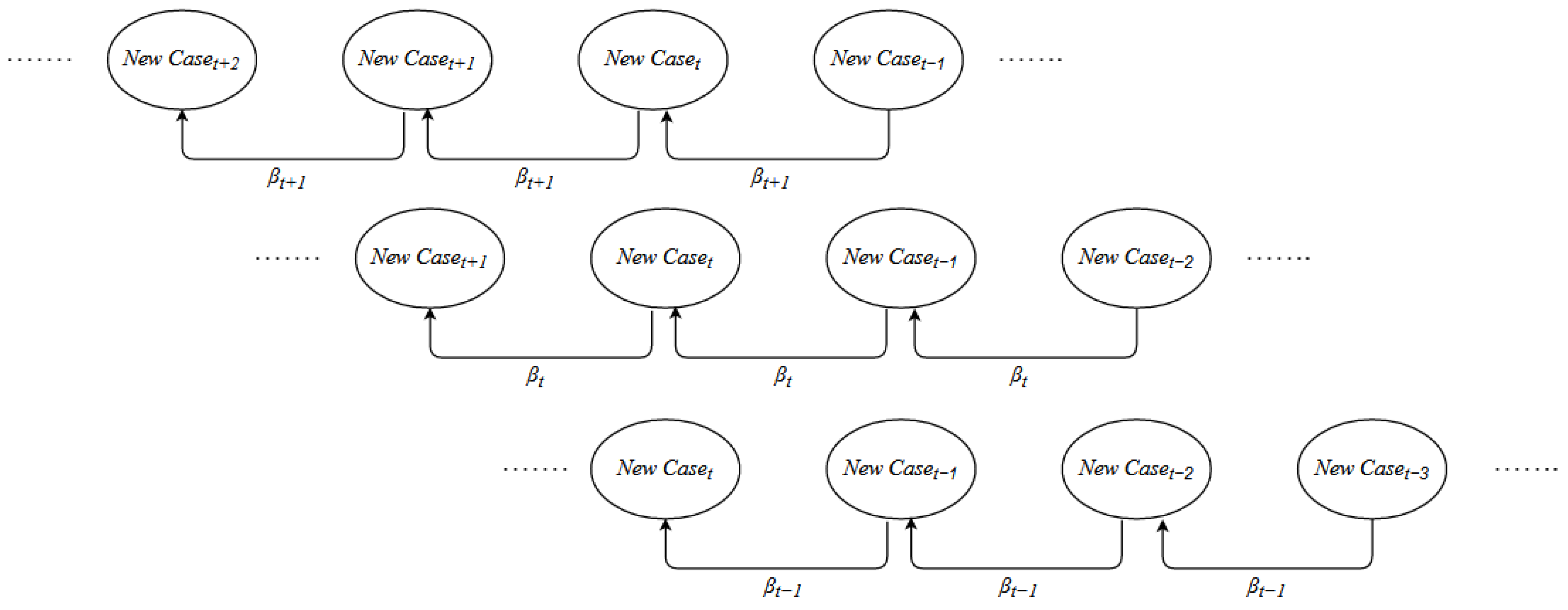
Figure 3.
COVID-19 transmission process diagram based on AR(1) model.

Figure 4.
White Noise Test results of residuals of the model. (The points never appear outside the confidence bands, the area between two black lines. The test statistic has a p-value of 0.8079, so we conclude that the process is not different from white noise).
Figure 4.
White Noise Test results of residuals of the model. (The points never appear outside the confidence bands, the area between two black lines. The test statistic has a p-value of 0.8079, so we conclude that the process is not different from white noise).

Figure 5.
COVID-19 Transmission Rate Calculated by the Model.


Table 1.
Definition of variables.
| Variable Type | Variable | Abbreviation |
|---|---|---|
| Explained variables | Hang Seng China Enterprises Index | HSCEI |
| SSE Composite Index | SSE | |
| Shenzhen Component Index | SZSE | |
| Explanatory variables | First-day COVID-19 Transmission Rate | NA |
| Second-day COVID-19 Transmission Rate | NA | |
| Control variables | Log(Gross Domestic Product of mainland China) | Log(GDP) |
| Log (money supply of mainland China) | logM2 | |
| Long-term Policy Interest Rate of The People’s Bank Of China | NA | |
| China Foreign Exchange Trading Center RMB Exchange Rate Index | CFETS RMB Exchange Rate Index | |
| Consumer Price Index of mainland China | CPI | |
| S&P 500 Index | SPX.GI | |
| NASDAQ Composite Index | IXIC.GI | |
| FTSE Singapore STI Index | STI.GI |
Table 2.
Descriptive statistics of variables in the model.
| Variable | N | Mean | SD | Max | Min | p50 | p95 | p5 |
|---|---|---|---|---|---|---|---|---|
| HSCEI | 985 | −2.90 × 10⁻⁴ | 7.35 × 10⁻³ | 5.12 × 10⁻² | −3.22 × 10⁻² | −1.46 × 10⁻⁴ | 1.11 × 10⁻² | −1.19 × 10⁻² |
| SSE | 985 | −9.70 × 10⁻⁵ | 4.96 × 10⁻³ | 2.41 × 10⁻² | −3.49 × 10⁻² | 1.28 × 10⁻⁴ | 7.39 × 10⁻³ | −8.55 × 10⁻³ |
| SZSE | 985 | 1.03 × 10⁻⁴ | 7.92 × 10⁻³ | 3.83 × 10⁻² | −1.86 × 10⁻² | −5.34 × 10⁻⁴ | 1.33 × 10⁻² | −1.14 × 10⁻² |
| First-day COVID-19 Transmission Rate | 985 | 8.11 × 10⁻¹ | 1.65 × 10⁻¹ | 1.45 | 2.08 × 10⁻¹ | 8.79 × 10⁻¹ | 9.859 × 10⁻¹ | 5.03 × 10⁻¹ |
| Second-day COVID-19 Transmission Rate | 985 | 1.28 × 10⁻¹ | 1.91 × 10⁻¹ | 7.92 × 10⁻¹ | −4.45 × 10⁻¹ | 0.00 | 4.97 × 10⁻¹ | 0,00 |
| LogGDP | 985 | 3.44 | 5.86 × 10⁻¹ | 3.54 | 3.29 | 3.45 | 3.53 | 3.30 |
| LogM2 | 985 | 4.36 | 1.16 × 10⁻¹ | 4.38 | 4.34 | 4.36 | 4.38 | 4.34 |
| Long-term Policy Interest Rate of The People’s Bank Of China | 985 | 1.95 | 3.82 × 10⁻¹ | 2.97 | 9.04 × 10⁻¹ | 1.94 | 2.65 | 1.26 |
| CFETS RMB Exchange Rate Index | 985 | 97.90 | 3.96 | 106.80 | 91.42 | 97.62 | 104.50 | 92.08 |
| CPI | 985 | 5.93 × 10⁻² | 4.81 × 10⁻² | 1.90 × 10⁻¹ | −1.88 × 10⁻² | 5.22 × 10⁻² | 1.68 × 10⁻¹ | −1.06 × 10⁻² |
| S&P 500 Index | 985 | 1.09 × 10⁻⁴ | 6.90 × 10⁻³ | 3.89 × 10⁻² | −5.54 × 10⁻² | 5.06 × 10⁻⁴ | 9.47 × 10⁻³ | −1.07 × 10⁻² |
| NASDAQ Composite Index | 985 | −9.40 × 10⁻⁵ | 4.50 × 10⁻³ | 2.56 × 10⁻² | −3.32 × 10⁻² | 5.40 × 10⁻⁵ | 6.12 × 10⁻³ | −6.78 × 10⁻³ |
| FTSE Singapore STI Index | 985 | 5.10 × 10⁻⁵ | 7.91 × 10⁻³ | 3.88 × 10⁻² | −5.71 × 10⁻² | 6.16 × 10⁻⁴ | 1.10 × 10⁻² | −1.25 × 10⁻² |
Table 3.
Results of panel data regression.
| OLS | Mixture Regression Model | Fixed Effects Model | |
|---|---|---|---|
| First-day COVID-19 Transmission Rate (t − 1) | −0.00538 *** | −0.00538 *** | −0.00538 *** |
| (−2.75) | (−2.75) | (−2.75) | |
| Second-day COVID-19 Transmission Rate (t − 2) | −0.00395 ** | −0.00395 ** | −0.00395 ** |
| (−2.24) | (−2.24) | (−2.24) | |
| Log(Real GDP) | 0.00779 * | 0.00779 * | 0.00779 * |
| (1.85) | (1.85) | (1.85) | |
| Log(M2) | 0.0762 * | 0.0762 * | 0.0762 * |
| (1.81) | (1.81) | (1.81) | |
| Long-term Policy Interest Rate | 0.000761 | 0.000761 | 0.000761 |
| (1.47) | (1.47) | (1.47) | |
| CFETS RMB Exchange Rate index | −0.000199 * | −0.000199 * | −0.000199 * |
| (−1.87) | (−1.87) | (−1.87) | |
| CPI | 0.0186 *** | 0.0186 *** | 0.0186 *** |
| (3.12) | (3.12) | (3.12) | |
| S&P 500 index | −0.0515 | −0.0515 | −0.0515 |
| (−0.92) | (−0.92) | (−0.92) | |
| NASDAQ Composite index | 0.0383 | 0.0383 | 0.0383 |
| (0.79) | (0.79) | (0.79) | |
| FTSE Singapore STI index | 0.458 *** | 0.458 *** | 0.458 *** |
| (16.37) | (16.37) | (16.37) | |
| 1.id | 0 | ||
| (.) | |||
| 2.id | −0.000393 | ||
| (−1.33) | |||
| 3.id | −0.000200 | ||
| (−0.68) | |||
| _cons | −0.337 * | −0.337 * | −0.337 * |
| (−1.93) | (−1.93) | (−1.93) | |
| N | 2955 | 2955 | 2955 |
t statistics in parentheses * p < 0.1, ** p < 0.05, *** p < 0.01.
Table 4.
Results of robustness test.
| HSCEI | SSE | SZSE | |
|---|---|---|---|
| First-day COVID-19 Transmission Rate (t − 1) | −0.00797 ** | ||
| (−2.48) | |||
| Second-day COVID-19 Transmission Rate(t−2) | −0.00636 ** | ||
| (−2.19) | |||
| L.First-day COVID-19 Transmission Rate (t − 1) | −0.00390 * | ||
| (−1.66) | |||
| L.Second-day COVID-19 Transmission Rate (t − 2) | −0.00187 | ||
| (−0.88) | |||
| L2.First-day COVID-19 Transmission Rate (t − 1) | −0.00648 * | ||
| (−1.68) | |||
| L2.Second-day COVID-19 Transmission Rate (t − 2) | −0.00502 | ||
| (−1.44) | |||
| Log(Real GDP) | −0.000472 | −0.0206 *** | 0.0387 *** |
| (−0.07) | (−4.03) | (4.58) | |
| Log(M2) | 0.265 *** | 0.180 *** | −0.187 ** |
| (3.84) | (3.57) | (−2.26) | |
| Long-term Policy Interest Rate | 0.00204 ** | 0.00140 ** | −0.000877 |
| (2.39) | (2.24) | (−0.86) | |
| CFETS RMB Exchange Rate Index | −0.000598 *** | −0.000225 * | 0.000243 |
| (−3.43) | (−1.77) | (1.16) | |
| CPI | 0.0380 *** | 0.00989 | 0.00798 |
| (3.89) | (1.38) | (0.68) | |
| S&P 500 Index | −0.323 *** | −0.0654 | 0.246 ** |
| (−3.50) | (−0.97) | (2.23) | |
| NASDAQ Composite Index | 0.358 *** | 0.0960 * | −0.348 *** |
| (4.50) | (1.65) | (−3.65) | |
| FTSE Singapore STI Index | 0.840 *** | 0.366 *** | 0.159 *** |
| (18.29) | (10.90) | (2.90) | |
| _cons | −1.095 *** | −0.693 *** | 0.665 * |
| (−3.80) | (−3.29) | (1.93) | |
| N | 985 | 984 | 983 |
t statistics in parentheses * p < 0.1, ** p < 0.05, *** p < 0.01.
Disclaimer/Publisher’s Note: The statements, opinions and data contained in all publications are solely those of the individual author(s) and contributor(s) and not of MDPI and/or the editor(s). MDPI and/or the editor(s) disclaim responsibility for any injury to people or property resulting from any ideas, methods, instructions or products referred to in the content. |
© 2023 by the authors. Licensee MDPI, Basel, Switzerland. This article is an open access article distributed under the terms and conditions of the Creative Commons Attribution (CC BY) license (https://creativecommons.org/licenses/by/4.0/).
Share and Cite
MDPI and ACS Style
Xiao, H.; Lin, D.; Li, S. Novel Method for Estimating Time-Varying COVID-19 Transmission Rate. Mathematics 2023, 11, 2383. https://doi.org/10.3390/math11102383
AMA Style
Xiao H, Lin D, Li S. Novel Method for Estimating Time-Varying COVID-19 Transmission Rate. Mathematics. 2023; 11(10):2383. https://doi.org/10.3390/math11102383
Chicago/Turabian StyleXiao, Hongfei, Deqin Lin, and Shiyu Li. 2023. "Novel Method for Estimating Time-Varying COVID-19 Transmission Rate" Mathematics 11, no. 10: 2383. https://doi.org/10.3390/math11102383
Note that from the first issue of 2016, this journal uses article numbers instead of page numbers. See further details here.