
An Adaptive Strategy for Medium-Term Electricity Consumption Forecasting for Highly Unpredictable Scenarios: Case Study Quito, Ecuador during the Two First Years of COVID-19


Abstract
:1. Introduction
Organization
2. Methodology
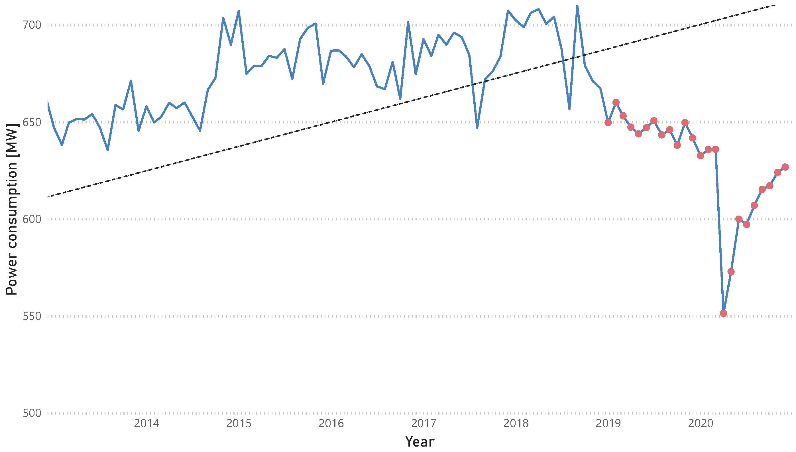
2.1. Case Study
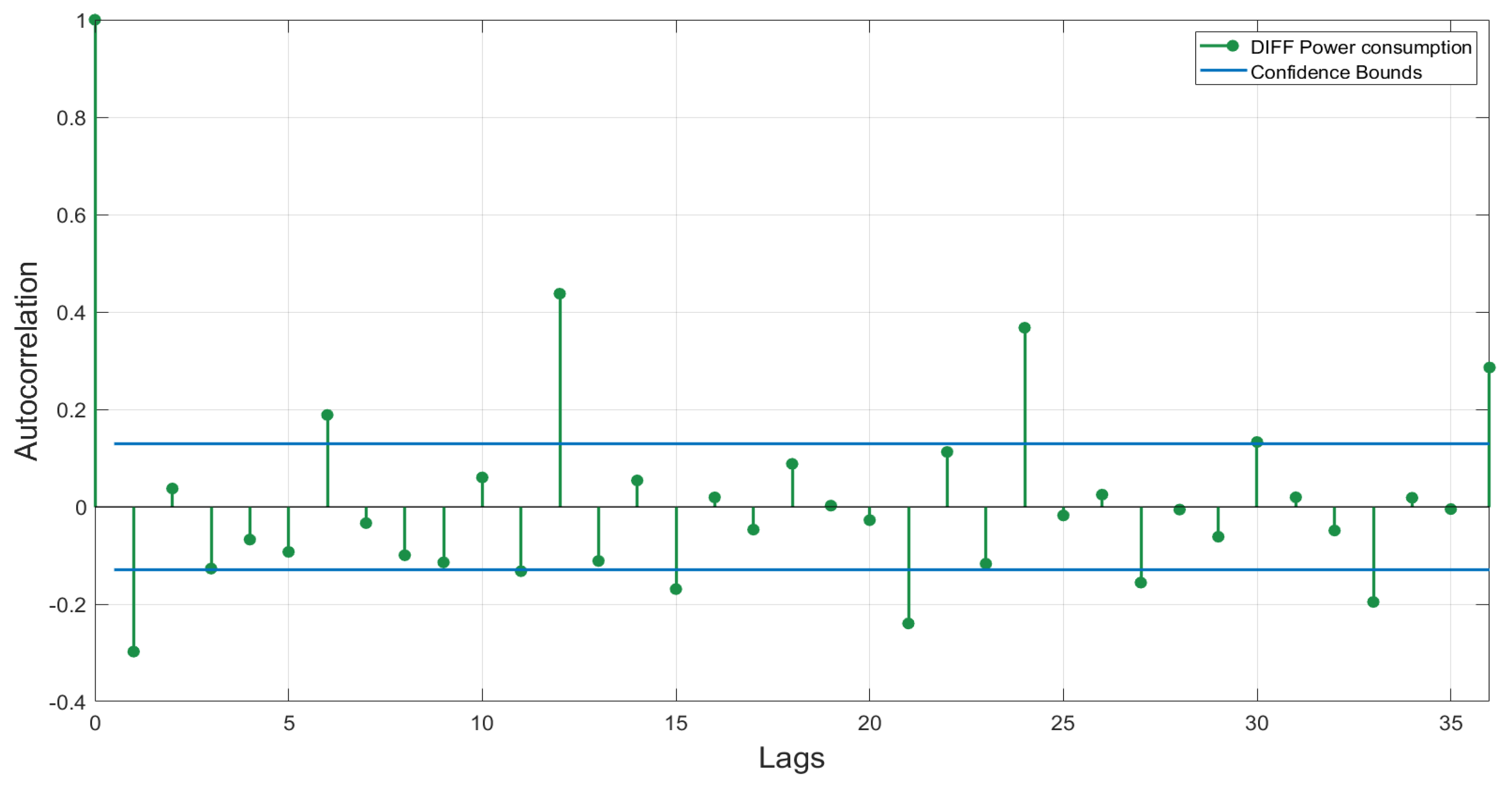
2.2. Time Series Analysis
2.2.1. Auto-Regressive Moving Average Time Series (ARMA)
2.2.2. Integrated Auto-Regressive Moving Average Time Series (ARIMA)
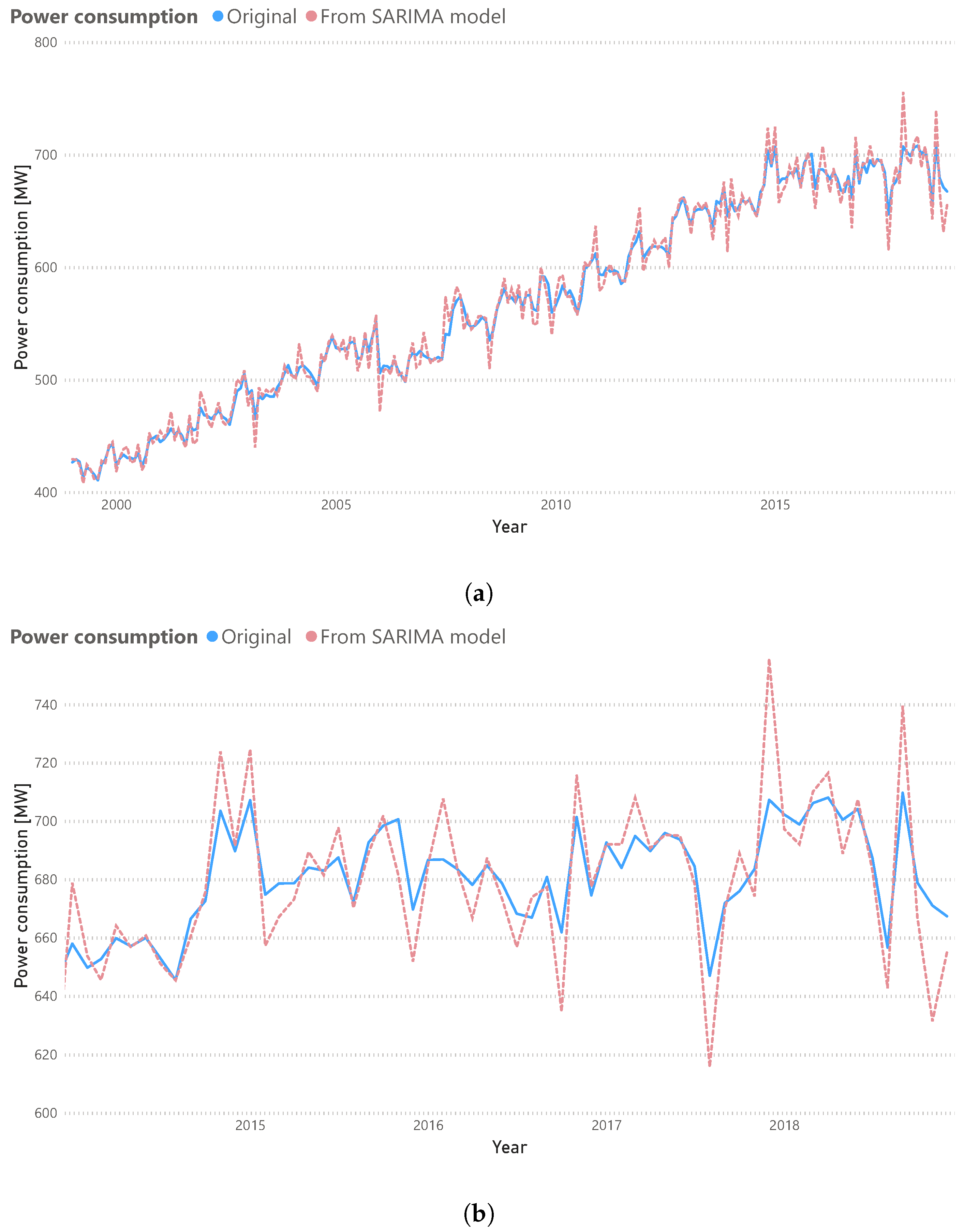
2.2.3. Seasonal Auto-Regressive Integrated Moving Average Time Series (SARIMA)
2.2.4. Based Model Analysis for SARIMA Coefficients
- Seasonal coefficient, .
- Differentiated coefficient, .
- Seasonal differentiated coefficient, .
- Auto-regressive coefficients, .
- Moving average coefficient, .
- Seasonal auto-regressive coefficients, .
- Seasonal moving average coefficient, .
2.3. Optimization Process: Particle Swarm Optimization
2.3.1. Cost Function
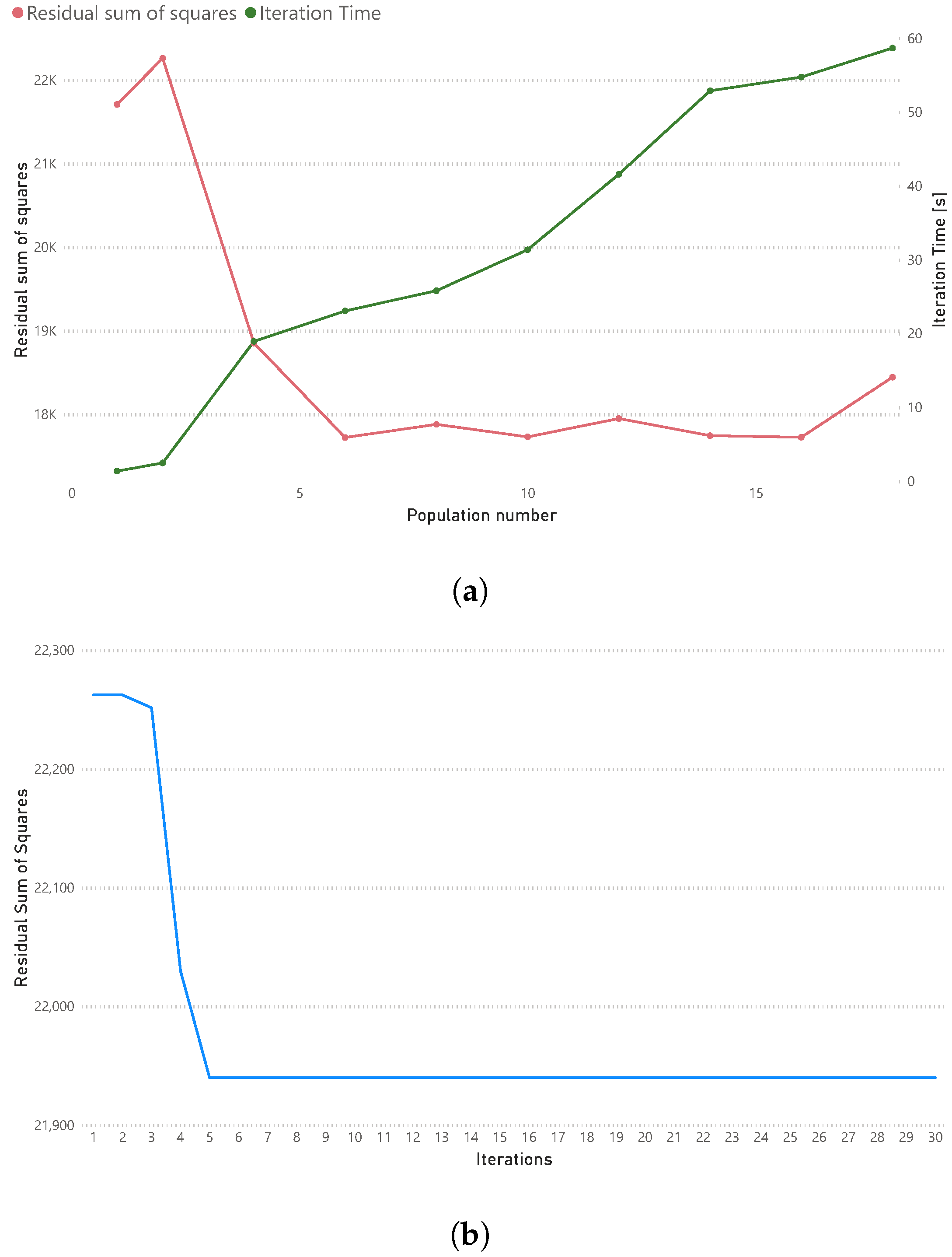
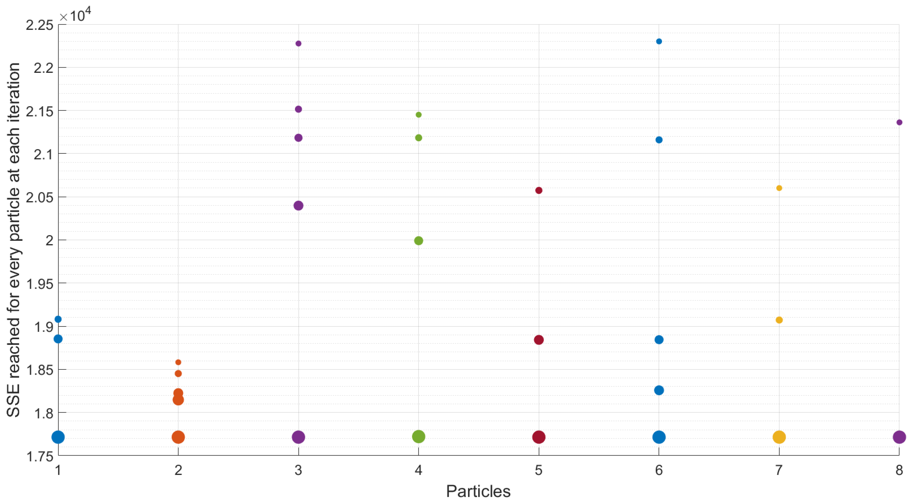
2.3.2. Number of Particles and Iterations for the Optimization Algorithm
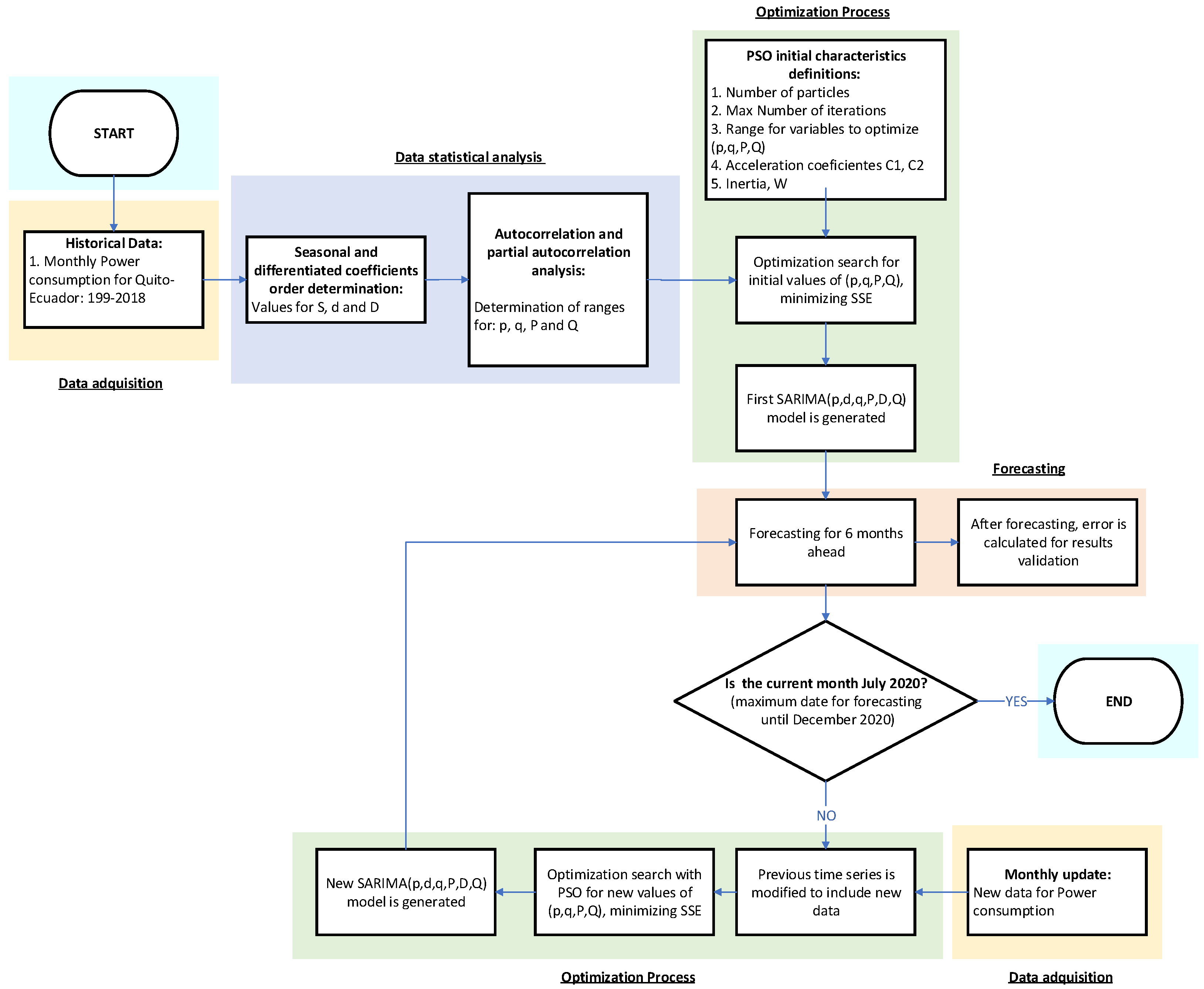
2.4. Methodology for Adaptive Forecasting of Electricity Consumption
3. Analysis of Results
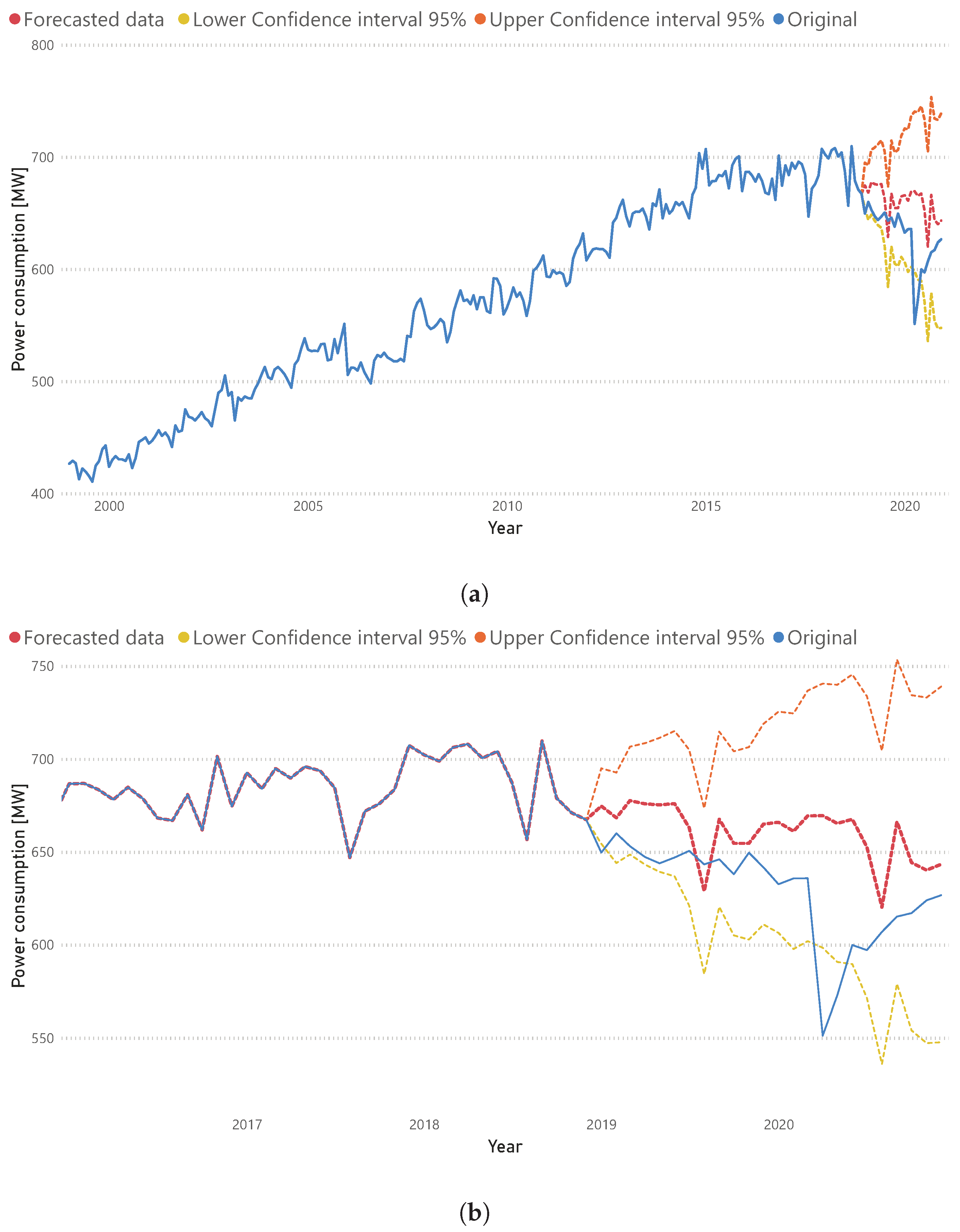
3.1. Traditional Approach for Forecasting
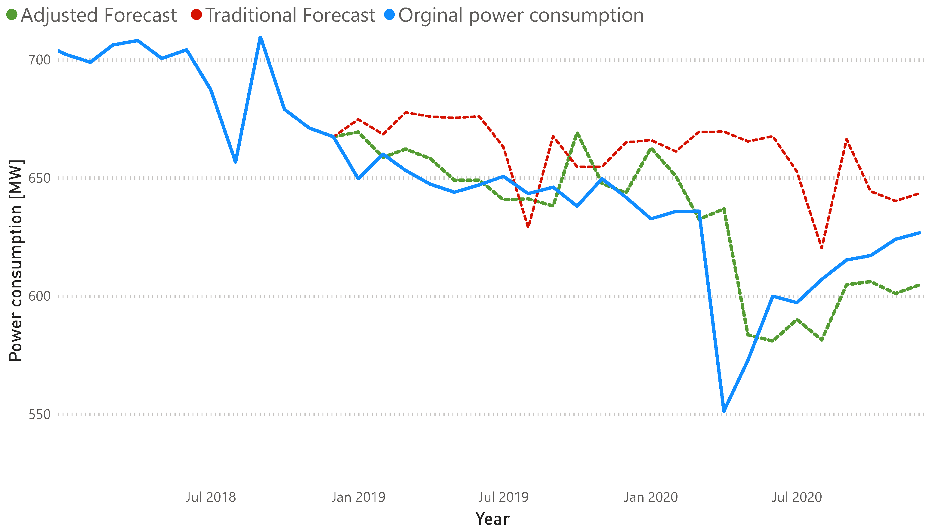
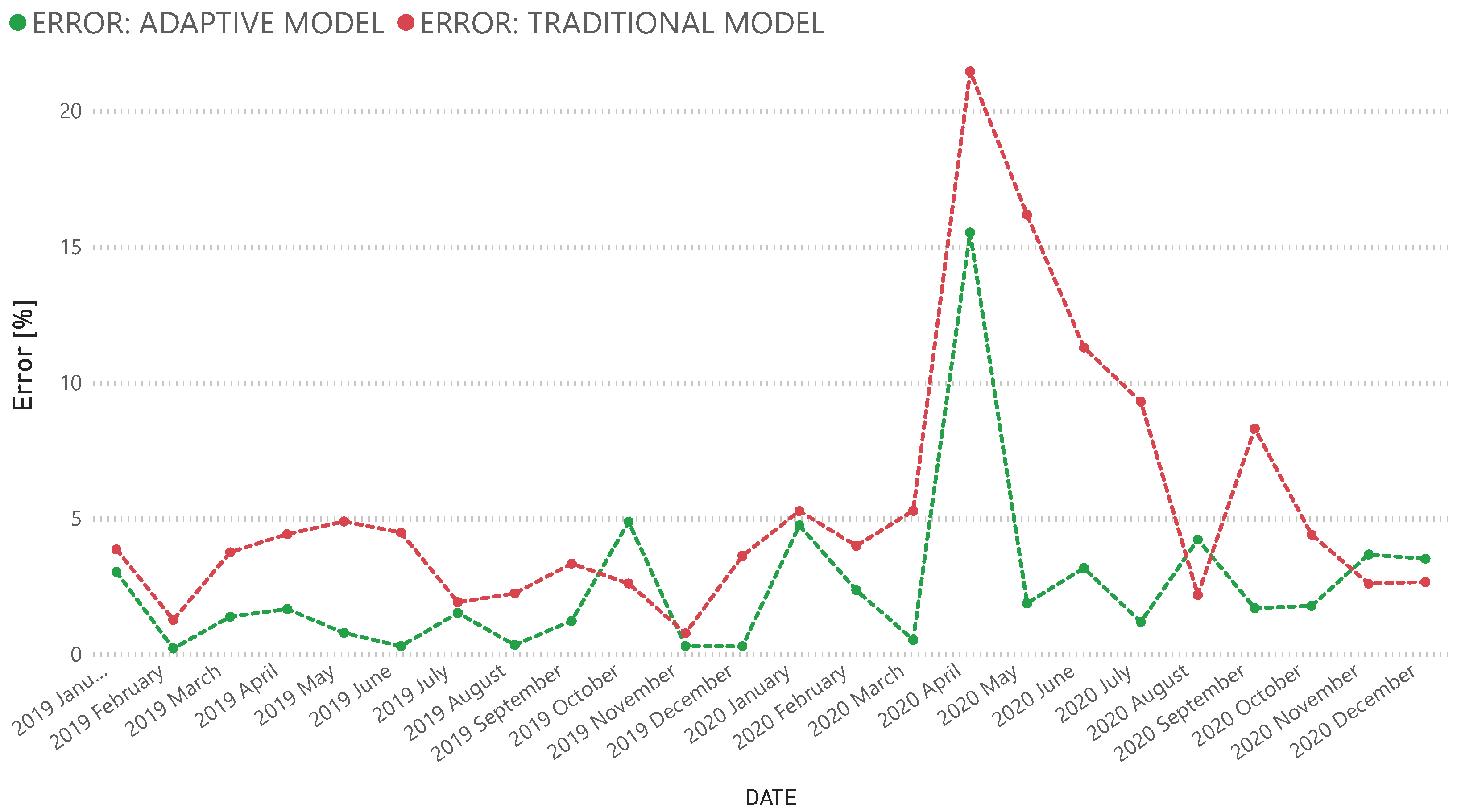
3.2. Adaptive Forecasting Approach for Power Consumption
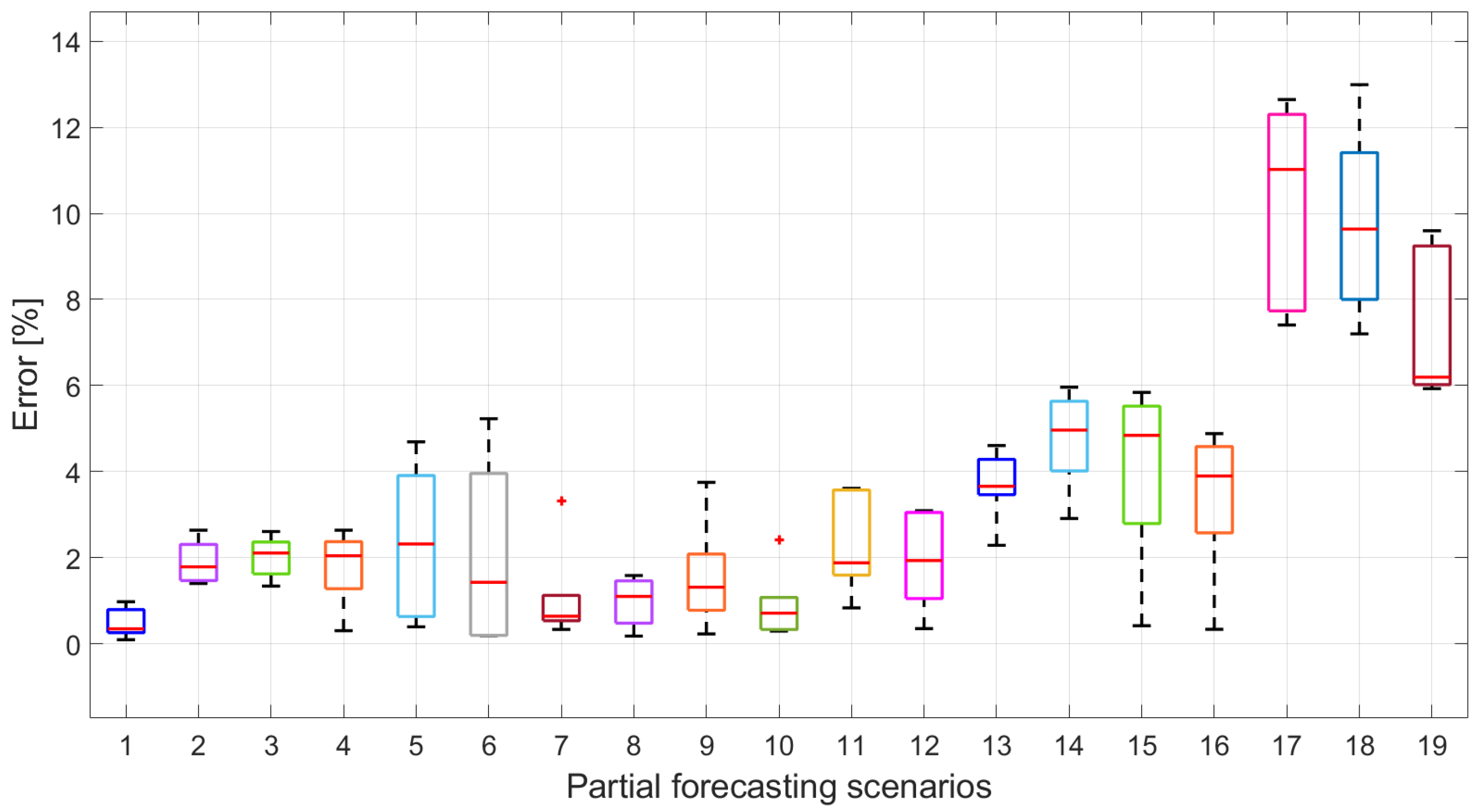
3.2.1. Results Achieved for Every Forecast Session
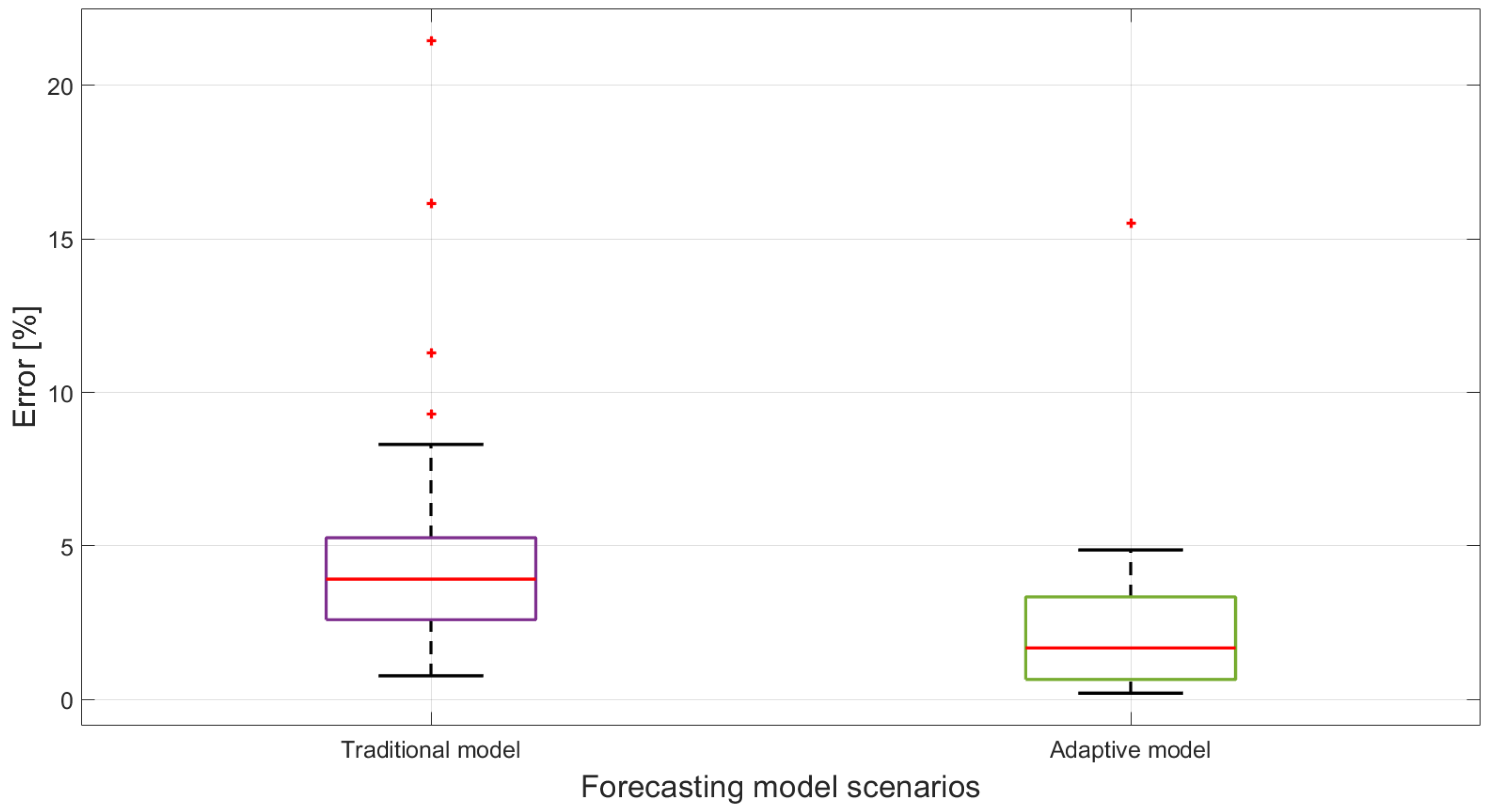
3.2.2. Global Results Achieved for 24 Months
4. Conclusions
Author Contributions
Funding
Data Availability Statement
Conflicts of Interest
Abbreviations
| Auto-regressive time series model | |
| Moving average time series model | |
| Auto-regressive moving average time series model | |
| Auto-regressive integrated moving average time series model | |
| Seasonal Auto-regressive integrated moving average time series model | |
| Artificial neural network | |
| Particle swarm optimization algorithm | |
| Differentiated time series | |
| Auto-correlation function | |
| Partial auto-correlation function | |
| Total number of models | |
| Partial auto-correlation function | |
| Time series component at time t | |
| White noise component at time t | |
| Coefficients for auto-regressive components | |
| Coefficients for moving average components | |
| Coefficients for seasonal auto-regressive components | |
| Coefficients for seasonal moving average components | |
| B | Back shift operator for time series |
| PSO algorithm speed at time t | |
| PSO algorithm position at time t | |
| w | PSO algorithm inertia coefficient |
| PSO algorithm personal acceleration coefficient | |
| PSO algorithm social acceleration coefficient | |
| Particle i best position at time t in PSO | |
| Global best position at time t in PSO | |
| Decimal random value for updated local position in PSO algorithm | |
| Decimal random value for updated global position in PSO algorithm | |
| Integer random value for updated local position in PSO algorithm | |
| Integer random value for updated global position in PSO algorithm | |
| Residual sum of squares | |
| Original electricity demand at position i |
References
- Bai, W.; Zhu, J.; Zhao, J.; Cai, W.; Li, K. An Unsupervised Multi-Dimensional Representation Learning Model for Short-Term Electrical Load Forecasting. Symmetry 2022, 14, 1999. [Google Scholar] [CrossRef]
- Gao, T.; Niu, D.; Ji, Z.; Sun, L. Mid-term electricity demand forecasting using improved variational mode decomposition and extreme learning machine optimized by sparrow search algorithm. Energy 2022, 261, 5328. [Google Scholar] [CrossRef]
- Zhuang, Z.; Zheng, X.; Chen, Z.; Jin, T.; Li, Z. Load Forecast of Electric Vehicle Charging Station Considering Multi-Source Information and User Decision Modification. Energies 2022, 15, 7021. [Google Scholar] [CrossRef]
- Mir, A.A.; Alghassab, M.; Ullah, K.; Khan, Z.A.; Lu, Y.; Imran, M. A review of electricity demand forecasting in low and middle income countries: The demand determinants and horizons. Sustainability 2020, 12, 5931. [Google Scholar] [CrossRef]
- Ur Rehman, S.A.; Cai, Y.; Fazal, R.; Walasai, G.D.; Mirjat, N.H. An integrated modeling approach for forecasting long-term energy demand in Pakistan. Energies 2017, 10, 1868. [Google Scholar] [CrossRef] [Green Version]
- Hussain, A.; Rahman, M.; Memon, J.A. Forecasting electricity consumption in Pakistan: The way forward. Energy Policy 2016, 90, 73–80. [Google Scholar] [CrossRef]
- Wang, Y.; Wang, J.; Zhao, G.; Dong, Y. Application of residual modification approach in seasonal ARIMA for electricity demand forecasting: A case study of China. Energy Policy 2012, 48, 284–294. [Google Scholar] [CrossRef]
- Jaramillo, M.; Tipán, L.; Muñoz, J. A novel methodology for optimal location of reactive compensation through deep neural networks. Heliyon 2022, 8, e11097. [Google Scholar] [CrossRef]
- Marwala, L.; Twala, B. Forecasting electricity demand in South Africa. In Proceedings of the 2014 International Joint Conference on Neural Networks (IJCNN), Beijing, China, 6–11 July 2014; pp. 3049–3055. [Google Scholar]
- Kumar, U.; Jain, V.K. Time series models (Grey-Markov, Grey Model with rolling mechanism and singular spectrum analysis) to forecast energy consumption in India. Energy 2010, 35, 1709–1716. [Google Scholar] [CrossRef]
- Panklib, K.; Prakasvudhisarn, C.; Khummongkol, D. Electricity Consumption Forecasting in Thailand Using an Artificial Neural Network and Multiple Linear Regression. Energy Sources Part B Econ. Plan. Policy 2015, 10, 427–434. [Google Scholar] [CrossRef]
- Yu, S.; Wang, K.; Wei, Y.M. A hybrid self-adaptive Particle Swarm Optimization-Genetic Algorithm-Radial Basis Function model for annual electricity demand prediction. Energy Convers. Manag. 2015, 91, 176–185. [Google Scholar] [CrossRef]
- Günay, M.E. Forecasting annual gross electricity demand by artificial neural networks using predicted values of socio-economic indicators and climatic conditions: Case of Turkey. Energy Policy 2016, 90, 92–101. [Google Scholar] [CrossRef]
- Hamzaçebi, C.; Es, H.A.; Çakmak, R. Forecasting of Turkey’s monthly electricity demand by seasonal artificial neural network. Neural Comput. Appl. 2019, 31, 2217–2231. [Google Scholar] [CrossRef]
- Kumar, A.; Yan, B.; Bilton, A. Machine Learning-Based Load Forecasting for Nanogrid Peak Load Cost Reduction. Energies 2022, 15, 6721. [Google Scholar] [CrossRef]
- Alsharekh, M.F.; Habib, S.; Dewi, D.A.; Albattah, W.; Islam, M.; Albahli, S. Improving the Efficiency of Multistep Short-Term Electricity Load Forecasting via R-CNN with ML-LSTM. Sensors 2022, 22, 6913. [Google Scholar] [CrossRef]
- Gobierno del Encuentro. Estadísticas del Sector Eléctrico Ecuatoriano Buscar. Available online: https://www.controlrecursosyenergia.gob.ec/estadisticas-del-sector-electrico-ecuatoriano-buscar (accessed on 31 October 2022).
- Gupta, A.; Kumar, A. Mid Term Daily Load Forecasting using ARIMA, Wavelet-ARIMA and Machine Learning. In Proceedings of the 2020 IEEE International Conference on Environment and Electrical Engineering and 2020 IEEE Industrial and Commercial Power Systems Europe (EEEIC/I&CPS Europe), Madrid, Spain, 9–12 June 2020. [Google Scholar]
- Sun, Y.; Liu, J. AQI Prediction Based on CEEMDAN-ARMA-LSTM. Sustainability 2022, 14, 2182. [Google Scholar] [CrossRef]
- Fu, C.; Jiang, S.F. A Hybrid Method for Structural Modal Parameter Identification Based on IEMD/ARMA: A Numerical Study and Experimental Model Validation. Appl. Sci. 2022, 12, 8573. [Google Scholar] [CrossRef]
- Zrieq, R.; Kamel, S.; Boubaker, S.; Algahtani, F.D.; Alzain, M.A.; Alshammari, F.; Alshammari, F.S.; Aldhmadi, B.K.; Atique, S.; Al-Najjar, M.A.A.; et al. Time-Series Analysis and Healthcare Implications of COVID-19 Pandemic in Saudi Arabia. Healthcare 2022, 10, 1874. [Google Scholar] [CrossRef] [PubMed]
- Tang, C.; Tao, X.; Wei, Y.; Tong, Z.; Zhu, F.; Lin, H. Analysis and Prediction of Wind Speed Effects in East Asia and the Western Pacific Based on Multi-Source Data. Sustainability 2022, 14, 2089. [Google Scholar] [CrossRef]
- Li, C.; Coster, D.C. Article Improved Particle Swarm Optimization Algorithms for Optimal Designs with Various Decision Criteria. Mathematics 2022, 10, 2310. [Google Scholar] [CrossRef]
- Alshamrani, A.M.; Alrasheedi, A.F.; Alnowibet, K.A.; Mahdi, S.; Mohamed, A.W. A Hybrid Stochastic Deterministic Algorithm for Solving Unconstrained Optimization Problems. Mathematics 2022, 10, 3032. [Google Scholar] [CrossRef]
- Sengupta, S.; Basak, S.; Peters, R. Particle Swarm Optimization: A Survey of Historical and Recent Developments with Hybridization Perspectives. Mach. Learn. Knowl. Extr. 2018, 1, 157–191. [Google Scholar] [CrossRef] [Green Version]
- Salameh, T.; Sayed, E.T.; Olabi, A.G.; Hdaib, I.I.; Allan, Y.; Alkasrawi, M.; Abdelkareem, M.A. Adaptive Network Fuzzy Inference System and Particle Swarm Optimization of Biohydrogen Production Process. Fermentation 2022, 8, 483. [Google Scholar] [CrossRef]
- Rokbani, N.; Abraham, A.; Alimi, A.M. Fuzzy Ant supervised by PSO and simplified ant supervised PSO applied to TSP. In Proceedings of the 13th International Conference on Hybrid Intelligent Systems (HIS 2013), Gammarth, Tunisia, 4–6 December 2013; pp. 251–255. [Google Scholar]
- Severino, A.G.V.; de Lima, J.M.M.; de Araújo, F.M.U. Industrial Soft Sensor Optimized by Improved PSO: A Deep Representation-Learning Approach. Sensors 2022, 22, 6887. [Google Scholar] [CrossRef]
- Zou, K.; Liu, Y.; Wang, S.; Li, N.; Wu, Y. A Multiobjective Particle Swarm Optimization Algorithm Based on Grid Technique and Multistrategy. J. Math. 2021, 2021, 1626457. [Google Scholar] [CrossRef]


| Number of Particles | Best RSS (Lowest) | Iteration Time [s] | Number of Iterations for Best RSS | Total Time until Best RSS [s] |
|---|---|---|---|---|
| 1 | 21,710 | 1.363 | 30 | 40.9 |
| 2 | 21,939.908 | 2.475 | 5 | 12.375 |
| 4 | 17,981.312 | 18.94 | 4 | 75.76 |
| 6 | 17,715.129 | 23.071 | 5 | 115.356 |
| 8 | 17,745.318 | 25.807 | 5 | 129.035 |
| 10 | 17,715.129 | 31.36 | 5 | 156.8 |
| 12 | 17,715.129 | 41.58 | 3 | 124.74 |
| 14 | 17,745.318 | 52.89 | 1 | 52.89 |
| 16 | 17,715.129 | 54.75 | 2 | 109.5 |
| 18 | 17,721.443 | 58.68 | 5 | 293.4 |
| Forecast Session | Best RSS Achieved | SARIMA Model | Average Error [%] |
|---|---|---|---|
| 1 | 17,715.129 | 0.4676 | |
| 2 | 18,017.779 | 1.8975 | |
| 3 | 18,027.888 | 2.0242 | |
| 4 | 19,271.434 | 1.7797 | |
| 5 | 18,228.642 | 2.3764 | |
| 6 | 18,248.905 | 2.0697 | |
| 7 | 18,286.459 | 1.0980 | |
| 8 | 18,372.007 | 0.9826 | |
| 9 | 18,529.698 | 1.5770 | |
| 10 | 18,893.479 | 0.9214 | |
| 11 | 18,929.334 | 2.2272 | |
| 12 | 18,957.999 | 1.9012 | |
| 13 | 17,715.129 | 3.6585 | |
| 14 | 19,253.160 | 4.7415 | |
| 15 | 17,745.318 | 4.0424 | |
| 16 | 17,981.312 | 3.3610 | |
| 17 | 26,061.050 | 9.3543 | |
| 18 | 17,745.318 | 9.8121 | |
| 19 | 17,715.129 | 7.1956 |
Publisher’s Note: MDPI stays neutral with regard to jurisdictional claims in published maps and institutional affiliations. |
© 2022 by the authors. Licensee MDPI, Basel, Switzerland. This article is an open access article distributed under the terms and conditions of the Creative Commons Attribution (CC BY) license (https://creativecommons.org/licenses/by/4.0/).
Share and Cite
Jaramillo, M.; Carrión, D. An Adaptive Strategy for Medium-Term Electricity Consumption Forecasting for Highly Unpredictable Scenarios: Case Study Quito, Ecuador during the Two First Years of COVID-19. Energies 2022, 15, 8380. https://doi.org/10.3390/en15228380
Jaramillo M, Carrión D. An Adaptive Strategy for Medium-Term Electricity Consumption Forecasting for Highly Unpredictable Scenarios: Case Study Quito, Ecuador during the Two First Years of COVID-19. Energies. 2022; 15(22):8380. https://doi.org/10.3390/en15228380
Chicago/Turabian StyleJaramillo, Manuel, and Diego Carrión. 2022. "An Adaptive Strategy for Medium-Term Electricity Consumption Forecasting for Highly Unpredictable Scenarios: Case Study Quito, Ecuador during the Two First Years of COVID-19" Energies 15, no. 22: 8380. https://doi.org/10.3390/en15228380