
The time series regression analysis in evaluating the economic impact of COVID-19 cases in Indonesia
Abstract
This study aims to determine the impact of COVID-19 cases in Indonesia on the USD/IDR exchange rate using the Transfer Function Model and Vector Autoregressive Moving-Average with Exogenous Regressors (VARMAX) Model. This paper uses daily data on the COVID-19 case in Indonesia, the USD/IDR exchange rate, and the IDX Composite period from 1 March to 29 June 2020. The analysis shows: (1) the higher the increase of the number of COVID-19 cases in Indonesia will significantly weaken the USD/IDR exchange rate, (2) an increase of 1% in the number of COVID-19 cases in Indonesia six days ago will weaken the USD/IDR exchange rate by 0.003%, (3) an increase of 1% in the number of COVID-19 cases in Indonesia seven days ago will weaken the USD/IDR exchange rate by 0.17%, and (4) an increase of 1% in the number of COVID-19 cases in Indonesia eight days ago will weaken the USD/IDR exchange rate by 0.24%.
1.Introduction
The world economic situation has deteriorated due to the increasing number of countries affected by the COVID-19 virus in the world such as America, Italy, and Spain. Trends in the number of patients and those who have died have not shown any decline even though the number of people who have recovered has increased compared to those who died. The impact of COVID-19 caused the exchange rates of several countries to fluctuate, for instance, Thai Baht, Mexican Peso, and Russian Ruble. The impact of COVID-19 hit Indonesian financial markets as well. Finance Minister Sri Mulyani said that Indonesia was quite affected by the spread of COVID-19, not only in the human health sector but also had disrupted the health of the global economy. The impact of this virus has resulted in various economic aspects; the stock exchange index fell, the USD/IDR exchange rate weakened drastically, MSME entrepreneurs struggled. Prior to the COVID-19 pandemic, the USD/IDR exchange rate was in the range of Rp 14,000.00 and during the pandemic, the Rupiah was briefly pressured down to the level of Rp 16,500.00. This COVID-19 pandemic caused panic in the global market, so investors withdrew their funds from Indonesia and placed them in a safe haven. This makes the USD/IDR exchange rate continue to weaken. The COVID-19 not only affects the USD/IDR exchange rate, but also has an impact on the decline in the IDX Composite to Rp 3,900.00. In addition, several countries also experienced the same thing, for example, SPI Singapore and SET Thailand. Therefore, it is interesting to see the impact of COVID-19 on the USD/IDR exchange rate and IDX composite.
The involvement of causal (external) factors into a time series can be viewed as part of a time series regression. Cryer and Chan (2006) consider it as intervention or outlier effects. If the external factor be the input and the response be the output series, then it can be a transfer function model (Box et al., 2016). Beside transfer function models, other name that are occasionally found in the related literature are distributed lag models (Lutkepohl, 2005). Many researches were conducted to model the cause-effect relationship among two or more time series. Nicholson et al. (2015) introduced VARX-L model to overcome the high-dimensional macroeconomic problem and Wei (2019) did a quantitative structural analysis to evaluate oil price shocks, economic policy uncertainty and China’s trade. Mukhaiyar et al. (2019) modeled the Dengue Fever Cases by considering the oulier factor using GSTAR(1;1) model meanwhile with the similar model Masteriana et al. (2019) used for analysis the Begal Criminal cases. By considering exogenous variable (average of monthly temperature) and outliers, Mukhaiyar et al. (2020) predict the monthly cases of dengue fever while Huda et al. (2020) used ADL model with outlier factor to do the prediction. Hasan et al. (2021) modeled the effect of COVID-19 pandemic on global economic, stock market, and the energy sector based on SVAR model, meanwhile Ganegoda et al. (2021) evaluated the interrelationship between daily COVID-19 cases and weather variables through temporal and spatial auto-correlation, and clustering-integrated panel regression. Saikhu et al. (2021) used ARIMA, bivariate and multivariate transfer function to predict COVID-19 cases. The effect of spatial dependence through railroad passenger’s mobility was considered by Pasaribu et al. (2021) to model the COVID-19 growth cases in Java island. More applications can be found in oscillation damping controllers of the power system (Liu et al., 2015), finance (Apriliandra et al., 2016), and residential building cost (Zhao et al., 2019) In this paper, the multivariate transfer function is explored to model the impact of the COVID-19 cases on the USD/IDR exchange rate and IDX composite, especially in the early days of the pandemic in Indonesia.
2.Methods
2.1The transfer function model
The transfer function model is a model describing the future predictive value of a time series (output series
Assume
where
(1)
where
2.2The VARMAX model
According to Wei (2006), the VARMA Model
where
Then the VARMA (1,1) SISO Model can be written in matrix form as follows:
Suppose
(2)
and
(3)
According to Eqs (2) and (3), the future value of
This also shows that
(4)
where
and
Equation (4) can be stated as:
where
where,
Thus, the VARMAX Model
Then suppose
(5)
Note that Eq. (2.2) is similar to the Transfer Function Model equation which has the order of the transfer function
Therefore, the univariate VARMAX Model
3.Data analysis
3.1Data analysis using the VARMAX model
In this section, the impact of COVID-19 cases in Indonesia is used to forecast the USD/IDR exchange rate and the IDX Composite. Suppose daily data of USD/IDR
Figure 1.
USD/IDR exchange rate vs the increase of COVID-19 cases time series plot (a) and IDX composite vs The Increase of COVID-19 Cases time series plot (b). It can be seen that as the number of COVID-19 cases in Indonesia increases, both the USD/IDR exchange rate and the IDX composite are weakening.
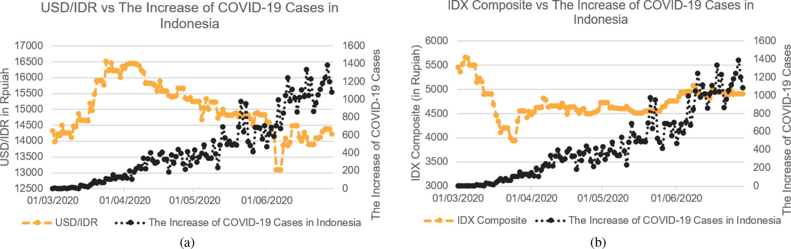
Table 1
Descriptive statistics of endogenous variables and exogenous variables
| Variables | T | Mean | Std. deviation | Minimum | Maximum |
|---|---|---|---|---|---|
|
| 121 | 14995 | 808.31 | 13085.4 | 16504 |
|
| 121 | 4725.1 | 314.7 | 3937.6 | 5650.1 |
|
| 121 | 455.3 | 376.2 | 0 | 1385 |
According to Table 1, it is known that the lowest USD/IDR exchange rate is Rp 13,085.40. This means that the strongest appreciation of the Rupiah is Rp 13,085.40 while the Rupiah depreciates the strongest at the level of Rp 16,504.80, namely on 24 March 2020 while the increase in the number of COVID-19 cases in Indonesia jumped by 107 cases. As the COVID-19 case in Indonesia has increased, investors have attracted their Rupiah to buy US dollars, as a result, the value of the Rupiah has weakened. The average USD/IDR exchange rate is Rp 14,995.31 with a standard deviation of 808.31.
The average IDX Composite value is Rp 4,725.1 and the highest value of the IDX Composite is Rp 5,650.14 meaning the strongest IDX Composite value is Rp 5,650.14 at 4 March 2020. However, after the strengthening of the IDX Composite on that date, the value of the IDX Composite continues to decline to below Rp 5,000.00 as cases of COVID-19 in Indonesia increase. It is also similar to the USD/IDR exchange rate, investors choose to invest in assets that are safer than placing their assets in shares in Indonesia, causing IDX Composite to touch the lowest level in history. It can be seen that, with the increase in COVID-19 cases in Indonesia, investors are shifting their assets to a safe haven, one of which is US dollars. The following is the movement of the two variables data displayed in the form of a time series plot.
The use of graphics in detecting that a series is stationary needs foresight so that the data stationarity test is performed using the Augmented Dickey-Fuller Test (ADF Test) with null hypotheses is “Data is not stationary” with alternative hypotheses is “Data is stationary”. The results are summarized in Table 2.
Table 2
Decision of the ADF test results. The USD/IDR exchange rate and the increase of COVID-19 cases are not stationary
| Variables | Decision | |
|---|---|---|
|
| 0.39 | Data is not stationary |
|
| 0.02 | Data is stationary |
|
| 0.11 | Data is not stationary |
According to Table 2, the USD/IDR exchange rate and the increase of COVID-19 cases both are not stationary for
Table 3
Sample correlation matrix function table for endogenous variable: (a) Before and (b) After differencing
| Schematic representation of cross correlations | |||||||||||||
| (a) Before differencing | |||||||||||||
| Variable/lag | 0 | 1 | 2 | 3 | 4 | 5 | 6 | 7 | 8 | 9 | 10 | 11 | 12 |
|
|
|
|
|
|
|
|
|
|
|
|
|
|
|
|
|
|
|
|
|
|
|
|
|
|
|
|
|
|
| (b) After differencing | |||||||||||||
| Variable/lag | 0 | 1 | 2 | 3 | 4 | 5 | 6 | 7 | 8 | 9 | 10 | 11 | 12 |
|
|
|
|
|
|
|
|
|
|
|
|
|
|
|
|
|
|
|
|
|
|
|
|
|
|
|
|
|
|
Based on Table 3(a), it can be seen that the (
It can be seen that the number of the (
It can be said that the (
Table 4
Partial autoregression matrix function table for endogenous variable after differencing
| Schematic representation of partial autoregression | ||||||||||||
|---|---|---|---|---|---|---|---|---|---|---|---|---|
| Variable/Lag | 1 | 2 | 3 | 4 | 5 | 6 | 7 | 8 | 9 | 10 | 11 | 12 |
|
|
|
|
|
|
|
|
|
|
|
|
|
|
|
|
|
|
|
|
|
|
|
|
|
|
|
|
It can be said that the value is between
Table 5
Minimum information criterion based on AICC. The possible models are AR(1) and MA(1)
| Minimum information criterion | ||||
| Lag | MA0 | MA1 | MA2 | MA3 |
| AR0 | 22.48 | 22.04 | 21.89 | 21.68 |
| AR1 | 20.13 | 20.05 | 20.12 | 20.12 |
| AR2 | 20.11 | 20.11 | 20.12 | 20.14 |
| AR1 | 20.15 | 20.16 | 20.16 | 20.15 |
Based on Table 5, model candidate can be chosen based on the smallest AICC value, namely VARMAX(1, 1, 1) Model with a value of 20.05. After obtaining the desired VARMAX Model, the next step is to estimate all the model parameters as follows:
The above equation can be formed in a mathematical equation:
1. For the USD/IDR exchange rate:
2. For IDX composite:
Since the unit of the response variables (USD/IDR exchange rate and IDX composite) are in IDR meanwhile the predictors (right-side of the equation) have various units, then the parameters coefficient will take the roles to adjust the unit. For example, the estimated parameter
After the VARMAX Model is selected, it will be checked whether the model is feasible or not to be predicted using the diagnostic test and the multivariate normal distribution at the residual.
1. The Portmenteau test
The Portmenteau test is used to test whether the residuals are identical and independent, using the following hypotheses formulation:
Take a look at the schematic representation of cross correlation of residuals on Table 6. It shows that the correlation only occurs at lag 0. It is supported by the Portmenteau test result which is for all lag times of the VARMAX(1, 1, 1) model’s residuals have
Table 6
Schematic representation of cross correlation of residuals table. Correlation only occurs at lag 0
Schematic representation of cross correlations of residuals Variable/Lag 0 1 2 3 4 5 6 7 8 9 10 11 12 2. The multivariate normal residual assumptions test.
The last stage of the diagnostic test is testing the multivariate normal distribution using the null hypotheses is “residual vector is multivariate normal distribution”. Using the chi-square test, the obtained
Since the
After obtaining the VARMAX model, then the next process is to predict USD/IDR exchange rate and the IDX Composite using the VARMAX(1, 1, 1) model for some time to come with
Table 7
The actual and prediction for the next 4 days along with the Upper Limit (UL) and Lower Limit (LL) with a 95% confidence interval for (a) USD/IDR exchange rate and (b) IDX composite
| Date of Y.2020 |
|
| 95% LL | 95% UL |
|
|---|---|---|---|---|---|
| (a) The USD/IDR exchange rate | |||||
| 30 June ( | 14470 | 14178.39 | 13727.39 | 14629.39 | 0.020 |
| 1 July ( | 14194.1 | 14143.66 | 13568.81 | 14718.51 | 0.003 |
| 2 July ( | 14187.9 | 14121.23 | 13456.87 | 14785.59 | 0.004 |
| 3 July ( | 14298.8 | 14109.07 | 13371.88 | 14846.25 | 0.010 |
| (b) The IDX Composite | |||||
| 30 June ( | 4950.39 | 4900.32 | 4717.94 | 5082.69 | 0.001 |
| 1 July ( | 4914.39 | 4895.44 | 4623.79 | 5167.07 | 0.003 |
| 2 July ( | 4966.78 | 4890.34 | 4556.90 | 5223.78 | 0.02 |
| 3 July ( | 4973.79 | 4885.14 | 4503.55 | 5266.73 | 0.02 |
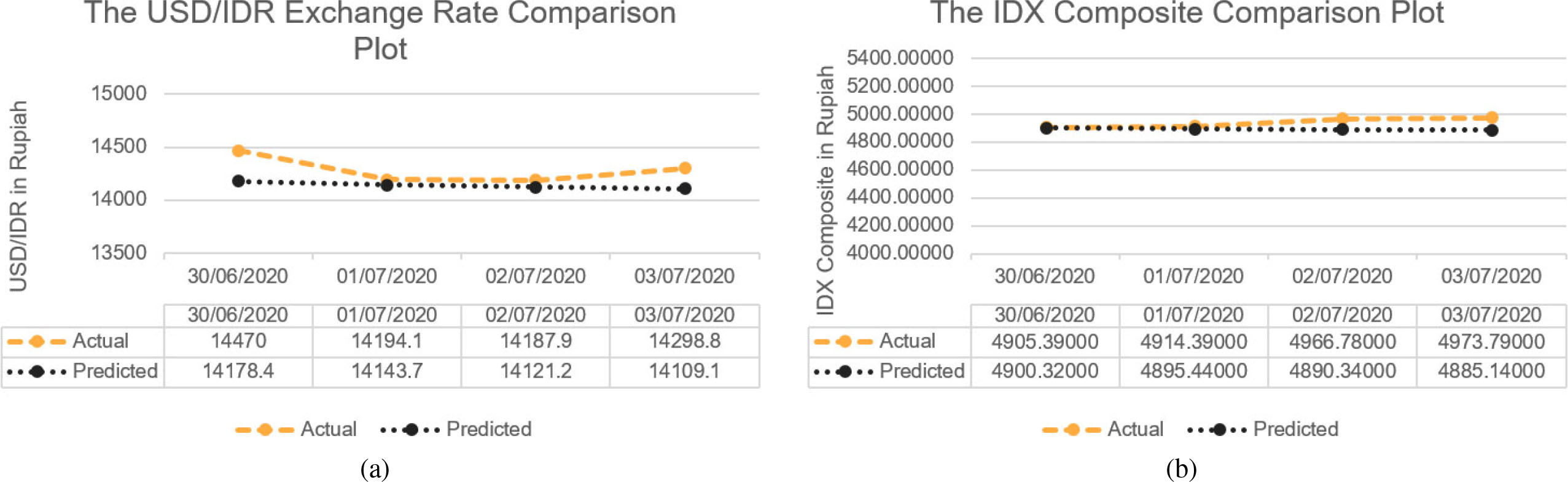
Based on Table 7(a) and (b), the prediction results for both USD/IDR exchange rate and IDX composite are still between the respective 95% lower limit and the 95% upper limit. The results of the absolute difference between the predicted value and the actual value divided by the actual value quite small for the next 4 days. This shows that the VARMAX (1, 1, 1) model for predicting the USD/IDR exchange rate and IDX composite is equally good. Likewise in Fig. 2a and b, the respective comparison plot looks quite close in value. In addition, its MAPE value is very good at 1.04% and 0.95% respectively. The predictive ability for the VARMAX(1, 1, 1) model is very good since the MAPE value is less than 10%.
Figure 2.
Comparison of Predicted Value and Actual Value for (a) The USD/IDR exchange rate, and (b) The IDX composite prediction. Both plots show the quite close of predicted and actual values.
3.2Data analysis using the transfer function model
An analysis of the impact of COVID-19 cases in Indonesia on the USD/IDR exchange rate using the transfer function model is being conducted here. Using the characteristic from the previous study above, the next step is to identify the ARIMA Model for the exogenous variable, namely, the increase of the number of COVID-19 cases in Indonesia. In the formation of the transfer function mModel, the basic assumption is stationary. Take a look at the ACF and PACF plots of the increase of the number of COVID-19 cases in Indonesia on the following Fig. 3.
Figure 3.
ACF and PACF Plot for the Exogenous Variable: (a) ACF and (b) PACF of original series, (c) ACF and (b) PACF of differenced series. Those plots are used to identify the suitable ARIMA Model.
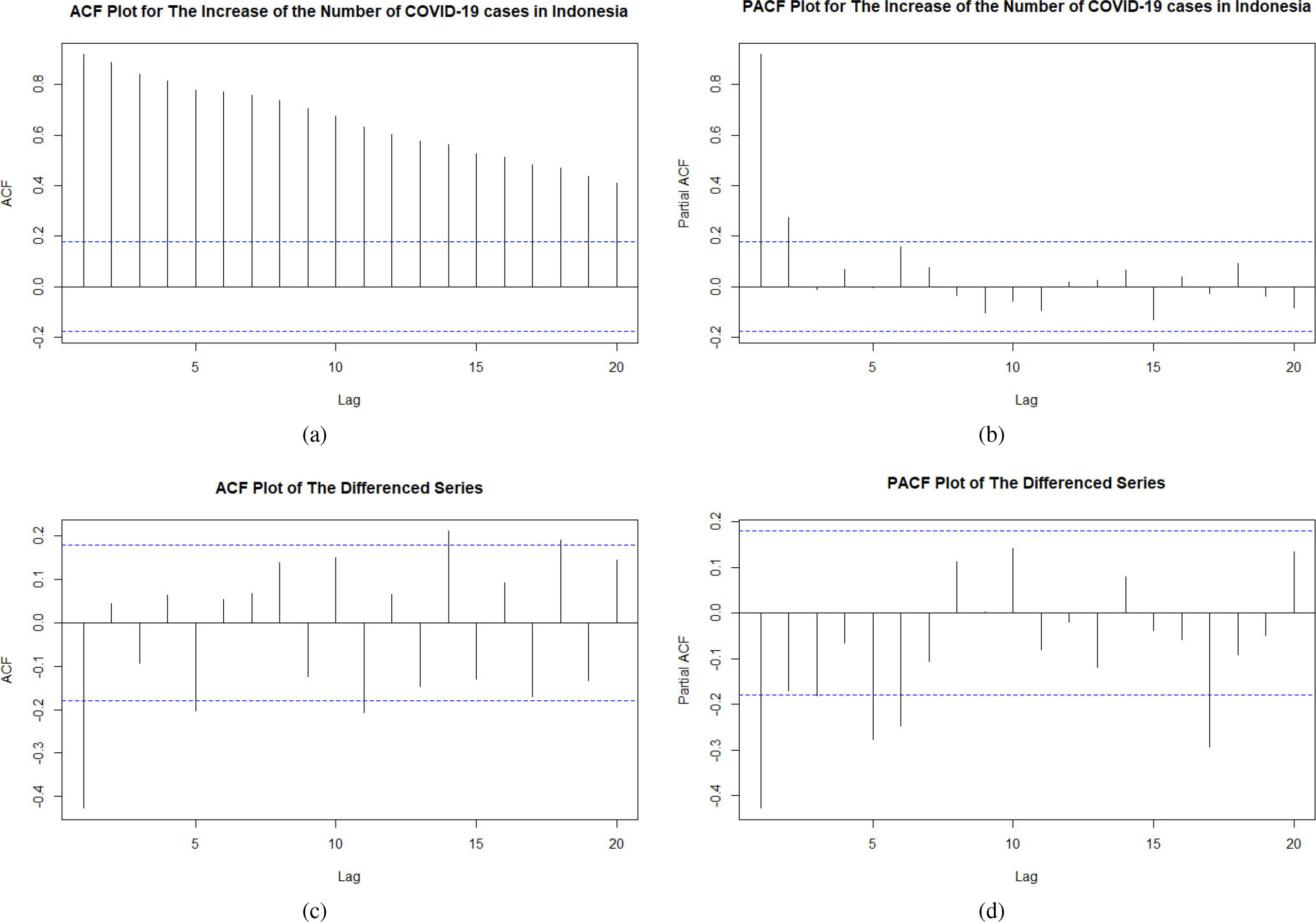
The two figures above show that the data is not stationary in the average since in Fig. 3a shows exponential decay. Therefore, to make the data is stationary in the average, it needs to be differenced first whose ACF and PACF are given by (c) and (d). From these figures, the ARIMA model can be determined based on the significant lag in the ACF and PACF plots. The ACF and PACF cut off at the first lag, thus the possible ARIMA Model for the exogenous variable are the ARIMA(1, 1, 1) model and the ARIMA(0, 1, 1) model.
The next step is the estimation and evaluation of both models parameters. To test the parameters significance, the null hypotheses is “exogenous variable is not significant” versus “exogenous variable is significant”. The estimators and its significance are presented on Table 8. In Table 8, parameter significance test has been performed for two possible models. The number in bold indicates that the parameter has
Table 8
The significance test of the todel parameters
| Variable | Parameter | Estimate | AIC | |
|---|---|---|---|---|
| ARIMA(1,1,1) |
| 0.09 | 0.49 | 1488.69 |
|
| ||||
| ARIMA(0,1,1) |
| 1487.12 |
After obtaining the suitable model, it is necessary to do a diagnostic test by conducting a white noise test and a residual normality test. The null hypotheses is “the residual is white noise” and vise versa for the alternative hypotheses. Based on the Ljung-Box test, it is found that only at 5’th lag the
Hereafter, the normality assumption of the ARIMA(0, 1, 1) residuals be checked through the QQ-Plot, as can be seen on Fig. 4. It shows that quite a lot of data values are along the normal line, so it can be said that the residuals are normally distributed.
Figure 4.
QQ-plot of residual ARIMA(0, 1, 1) model. It can be seen that the ARIMA(0, 1, 1) model meets the normality assumption because of the large amount of data values are along the lines.
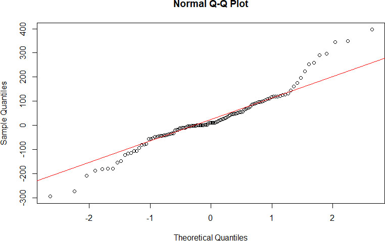
Since by seeing the QQ-Plot is considered to be less objective, another test is carried out to check whether the residuals are normally distributed using the Jarque Bera test with the null hypothesis is “residual is not normally distributed”. It is obtained that the
Based on the estimated parameter values in Table 8, the model can be written as:
The pre-whitening process for the exogenous series is
such that the pre-whitening process for the output endogenous series is,
The pre-whitening step in the exogenous series must also be executed in the endogenous series. This is for maintaining the integrity of the functional relationship of the transfer function maps
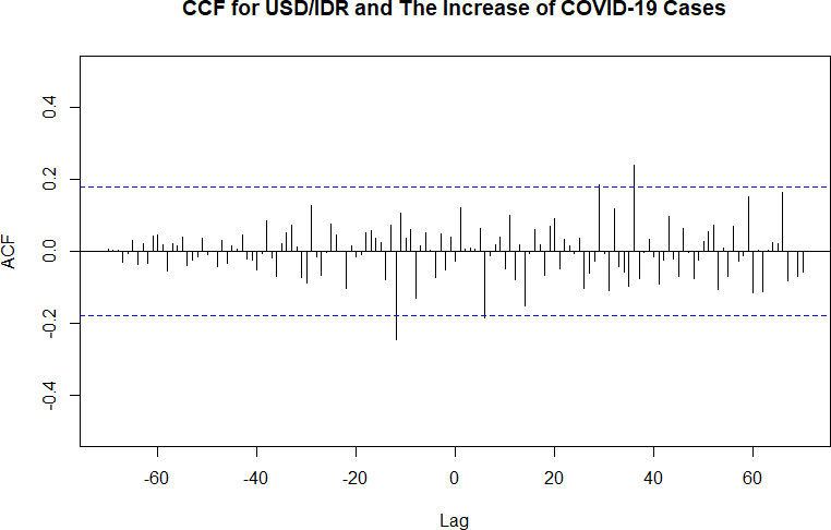
In order to obtain the transfer function model, the Crosscorrelation Function (CCF) should be investigated. The CCF is used to determine the value of the main order of the transfer function, namely order
Figure 5.
CCF plot of the pre-whitened exogenous and pre-whitened endogenous variable. It can be seen that the main order of the transfer function is (
The estimated parameters of the transfer function with order
Next, the ARMA modeling will be performed on the noise series so that the white noise residual will be obtained. The ACF and PACF plot of residuals are presented in Fig. 6. Based on this plot, the possible model obtained is MA(1).
Thereafter, all parameters of the transfer function model are estimated and obtained that
and be simplified into the following form:
After obtaining the transfer function model, it is necessary to do a diagnostic test between
Further, the crosscorrelation test is carried out using the null hypotheses is “
Table 9
The USD/IDR exchange rate prediction for the next 4 days along with the upper and lower limits with a 95% confidence limits
| Date of Y.2020 |
|
| 95% LL | 95% UL |
|
|---|---|---|---|---|---|
| 30 June ( | 14470 | 14260.30 | 13783.08 | 14737.58 | 0.01 |
| 1 July ( | 14194.1 | 14294.60 | 13651.19 | 14937.98 | 0.007 |
| 2 July ( | 14187.9 | 14320.79 | 13546.10 | 15095.48 | 0.009 |
| 3 July ( | 14298.8 | 14347.51 | 13460.75 | 15234.26 | 0.003 |
Figure 6.
ACF dan PACF plot of the residual. The identified time series model from the ACF and PACF plot is MA(1).
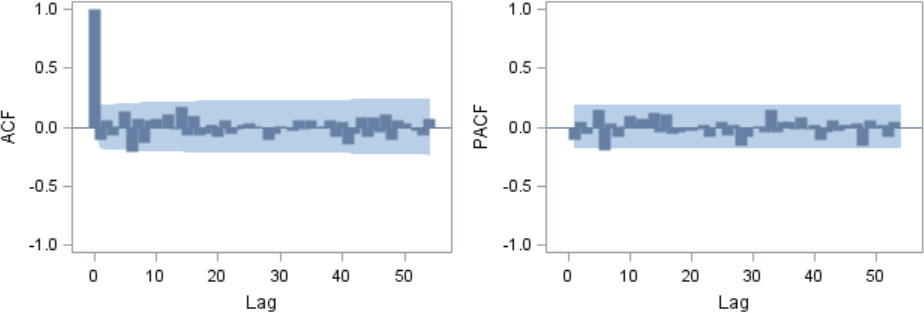
Figure 7.
The residual normality test. The graph shows that the residuals are normally distributed.
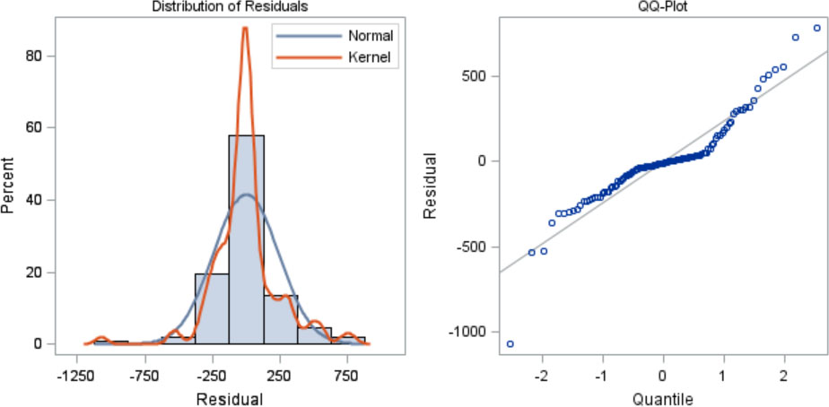
Figure 7 shows that quite a lot of data values are along the normal line, so it can be said that the residuals are normally distributed. Thus, the next step is to predict the USD/IDR exchange rate with
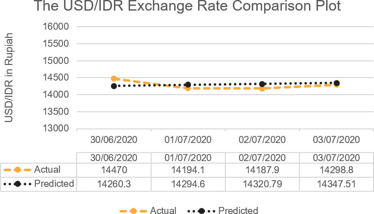
Based on Table 9, the prediction results are still between the 95% lower limit and the 95% upper limit and also the results of the absolute difference between the predicted value and the actual value divided by the actual value quite small for the next 4 days. This shows that the transfer function model for predicting the USD/IDR exchange rate is quite good. Likewise in Fig. 8, the comparison plot looks quite close in value. In addition, its MAPE value is very good at 0.86%. The predictive ability for the transfer function model is very good since the MAPE value is lower 10%.
Figure 8.
Comparison of predicted value and actual value. The USD/IDR exchange rate prediction are quite close from the actual value.
4.Discussion
On Section 3, two case studies were conducted using different approaches. First, the VARMAX model is used to model the prediction of the USD/IDR exchange rate and the IDX composite which are influenced by the increase of the number of COVID-19 cases in Indonesia. Here, prediction of the USD/IDR is not only be influenced by the increase of the number of COVID-19 cases in Indonesia, but also by the IDX composite. Here are the final model:
1. For the USD/IDR exchange rate:
This means that intercept will make the USD/IDR exchange rate today depreciate at Rp 3154.92. Then an increase of 1% in the number of COVID-19 cases in Indonesia will weaken the USD/IDR exchange rate by 0.08%. A 1% increase in the yesterday’s number of COVID-19 cases in Indonesia will strengthen the USD/IDR exchange rate by 0.23%. Furthermore, an increase of 1% in the yesterday’s USD/IDR exchange rate will make the USD/IDR exchange rate depreciate today by 0.87%, while an increase of 1% in the yesterday’s IDX Composite will make the USD/IDR exchange rate appreciate today by 0.23%.
2. For IDX composite:
This means that the intercept will make the IDX composite increase by Rp 66.47 today. Then an increase of 1% in the number of COVID-19 cases in Indonesia will make the IDX composite today decrease by 0.003%. An increase of 1% in the yesterday’s number of COVID-19 cases in Indonesia will make the IDX composite today increase by 0.007%. Furthermore, an increase of 1% in the yesterday’s USD/IDR exchange rate will make the IDX composite increase today by 0.007%, while an increase of 1% in the yesterday’s IDX Composite will make the IDX composite today increase by 0.96%.
From diagnostic checking of residuals, the multivariate normal assumption could not be fulfilled. It becomes the weakness of this model. When it is used for predicting, it is obtained that the MAPE value for the USD/IDR exchange rate is 1.04% which means that the model has a great predictive ability. As a matter of fact, from the comparison plot, it can be seen that the prediction for 1 July 2020 and 2 July 2020 is pretty close with the actual values.
Second, the transfer function model is used to model the prediction of the USD/IDR exchange rate. In this case, it was assumed that the USD/IDR exchange rate only be influenced by the increase of the number of COVID-19 cases in Indonesia. The final model is:
This means that an increase of 1% in the number of COVID-19 cases in Indonesia six days ago will weaken the USD/IDR exchange rate by 0.003%. A 1% increase in the number of COVID-19 cases in Indonesia seven days ago will also weaken the USD/IDR exchange rate by 0.17%. Furthermore, an increase of 1% in the number of COVID-19 cases in Indonesia eight days ago will make the USD/IDR exchange rate today depreciate by 0.24%.
As consequence, the MAPE value for the USD/IDR exchange rate is 0.86% which means that the model has a great predictive ability. In fact, from the comparison plot, it can be seen that the last three predicted values are very close to the actual values. Based on these results, the USD/IDR exchange rate is better to be predicted using the transfer function model since it has lower MAPE value than using the VARMAX Model.
5.Conclusion and remark
According to Section 3, it can be concluded that the increase of the number of COVID-19 cases in Indonesia significantly affected the USD/IDR exchange rate. The findings in detail can be explained as follows:
1. The higher the increase of the number of COVID-19 cases in Indonesia will have an impact on the increasingly depreciating value of the USD/IDR exchange rate.
2. An increase of 1% in the number of COVID-19 cases in Indonesia six days ago will weaken the USD/IDR exchange rate by 0.003%.
3. An increase of 1% in the number of COVID-19 cases in Indonesia seven days ago will weaken the USD/IDR exchange rate by 0.17%.
4. An increase of 1% in the number of COVID-19 cases in Indonesia eight days ago will weaken the USD/IDR exchange rate by 0.24%.
Acknowledgments
The authors thank to the RISTEK/BRIN grant, “Penelitian Dasar Unggulan Perguruan Tinggi (PDUPT)”, 2019–2021 for supporting funds. Our gratitude for the reviewers of this manuscript.
References
[1] | Andayani, N., Sumertajaya, I. M., Ruchjana, B. N. & Aidi, M. N. ((2016) ). Comparison ARIMA-X and VARMA-X model to space time data: A case study of rice price in six provinces on java island, International Journal of Applied Mathematics and Statistics, 55: (3). |
[2] | Apriliandara, M., Suhartono, & Prastyio, D. D. ((2016) ). VARI-X model for currency inflow and outflow forecasting with Eid Fitr effect in Indonesia, AIP Conference Proceedings, 1746: (1), 020041. |
[3] | Box, G. E. P., Jenkins, G. M. & Reisel, G. C., and Ljung, G. M. ((2016) ). Time Series Analysis. Forecasting and Control, 5 |
[4] | Cryer, J. & dan Kung-Sik Chan D. ((2008) ). Time Series Analysis: With Apllication in R Second Edition. Springer. |
[5] | Ganegoda, N. C., Wijaya, K. P. & Amadi, M., Erandi, K. K. W. H. & Aldila, D. ((2021) ). Interrelationship between daily COVID-19 cases and average temperature as well as relative humidity in Germany, Scientific Reports, 11: (1). |
[6] | Hasan M. B., Mahi, M., Sarker, T. & Amin, M. R. ((2021) ). Spillovers of the COVID-19 Pandemic: Impact on global economic activity, the stock market, and the energy sector, Journal of Risk and Financial Management, 14: (5): 1-19. |
[7] | Huda, N. M., Mukhaiyar. Forecasting dengue fever cases using autoregressive distributed lag model with outlier factor, AIP Conference Proceedings, 2268: (1), 020005. |
[8] | Liu, H., Zhu, L., Pan, Z., Ba, F., Liu, Y., Liu, Y., Patel, M., Farantatos, E. & Bhatt, N. ((2015) ). ARMAX-based transfer function model identification using wide-area measurement for adaptive and coordinated damping control, IEEE Transactions on Smart Grid, 8: (3), 020005. |
[9] | Lutkepohl, H. ((2005) ). New Introduction to Multiple Time Series Analysis. Springer. |
[10] | Masteriana, D., Riani, M. I. & Mukhaiyar, U. ((2019) ). Generalized STAR (1; 1) model with outlier-case study of begal in Medan, North Sumatera, Journal of Physics: Conference Series, 1245: (1), 012046. |
[11] | Mukhaiyar, U., Huda, N. M. & Pasaribu, U. S. ((2020) ). Analysis of generalized space time autoregressive with exogenous variable (GSTARX) model with outlier factor, Journal of Physics: Conference Series, 1496: (1), 012004. |
[12] | Mukhaiyar, U., Huda, N. M., Sari, K. N. & Pasaribu, U. S. ((2019) ). Modeling dengue fever cases by using GSTAR (1; 1) model with outlier factor, Journal of Physics: Conference Series, 1366: (1), 01122. |
[13] | Nicholson, W., Matteson, D. S. & Bien, J. ((2015) ). VARX-L: Structured regularization for large vector autoregressions with exogenous variables, International Journal of Forecasting, 33: (3). |
[14] | Pasaribu, U. S., Mukhaiyar, U., Huda, N. M., Sari, K. N. & Indratno, S. W. ((2021) ). Modelling COVID-19 growth cases of provinces in java Island by modified spatial weight matrix GSTAR through railroad passenger’s mobility, Heliyon, 7: (2), e0602. |
[15] | Saikhu, A., Hudiyanti, C. V., Buliali, J. L. & Hariadi, V. ((2020) ). Predicting COVID-19 confirmed case in surabaya using autoregressive integrated moving average, bivariate and multivariate transfer function, IOP Conf. Series: Materials Science and Engineering, 1077: (2021), 012055. |
[16] | Spliid, H. ((1983) ). A fast estimation method for the vector autoregressive moving average model with exogenous variables. Technical University of Denmark Press. |
[17] | Tsay, R. S. ((2014) ). Multivariate time series analysis with R and financial applications. Wiley. |
[18] | Wei, W. W. S. ((2006) ). Time series analysis: Univariate and multivariate method. Pearson. |
[19] | Wei, Y. ((2019) ). Oil price shocks, economic policy uncertainty and China’s trade: A quantitative structural analysis, The North American Journal of Economics and Finance, 48: : 20-31. |
[20] | Widyanti, D. ((2020) ). Pemodelan regresi deret waktu univariat dan multivariat menggunakan model fungsi transfer dan vektor autoregressive moving average with exogenous regressors. Tugas Akhir Program Sarjana Matematika. Institut Teknologi Bandung. |
[21] | Zhao, L., Mbachu, J., Liu, Z. & Zhang, H. ((2019) ). Transfer function analysis: Modelling residential building costs in new zealand by including the influences of house price and work volume, MDPI: Buildings, 9: (152). |
[22] | References from Sites (website): The USD/IDR exchange rate and the IDX Composite Data 1 March 2020–3 July 2020, data obtained through internet sites: https://finance.yahoo.com/quote/USDIDR%3DX/history?period1=1551657600&period2=1583798400&interval=1d&filter=history&frequency=1d. |

