
Analysis of Systemic Risk Scenarios and Stabilization Effect of Monetary Policy under the COVID-19 Shock and Pharmaceutical Economic Recession
Department of Economics, Sejong University, Seoul 05006, Gwangjin-gu, Republic of Korea
*
Author to whom correspondence should be addressed.
Sustainability 2023, 15(1), 880; https://doi.org/10.3390/su15010880
Submission received: 23 November 2022
/
Revised: 15 December 2022
/
Accepted: 27 December 2022
/
Published: 3 January 2023
(This article belongs to the Special Issue The Role and Impact of the Internet of Things (IoT) in Sustainable Smart Cities)
Abstract
:The Global Financial Crisis (GFC) will cause turbulence in the pharmaceutical market and the stagnation of market liquidity, leading to a deep recession in the pharmaceutical economy. After the COVID-19 outbreak, the pharmaceutical economic recession and the rising pharmaceutical financial crisis caused by the closure and control of the COVID-19 outbreak in China were important reasons for the accumulation of systemic financial risks in China. To realize the pharmaceutical economy and financial stability, this paper studies the weakening mechanism of the stabilization effect in systemic risk scenarios and analyzes how the evolution of systemic risk under the COVID-19 shock affects the stabilization effect of monetary policy. Under the COVID-19 shock, in the stage of falling China Financial Stress Index (CFSI), the systemic risk is relatively low, and the impact of traditional policy on macroeconomic stability is more significant; in the rising stage of CFSI, the systemic risk is relatively high, and the impact of traditional policy on macroeconomic stability is limited. This paper develops a Time-Varying Modified CRITIC weighting method and constructs a Time-Varying CFSI. This paper identifies systemic risk scenarios under the COVID-19 shock based on the Markov-Switching Mean Heteroskedastic Vector Auto-Regressive (MSMH-VAR) model and evaluates the stabilizing effects of monetary policy in different economic and financial regional systems (normal times and systemic risk scenarios). The results show that in normal times, loose monetary policy increases price levels, and tight monetary policy reduces price levels with a time lag. In systemic risk scenarios under the COVID-19 shock, the easing effect of policy on output growth is relatively small, and tighter policy increases output growth and prices in the short run and increases volatility in output growth and price levels in the long run. That is, under the COVID-19 shock in systemic risk scenarios, it is difficult to achieve stable growth and stable prices with monetary policy, and the stabilization effect is weakened. This paper focuses on the relationship between systemic risks, monetary policy, and output stability under the COVID-19 shock, analyzes the weakening of stabilization effects after the crisis, and expands the theoretical path of monetary policy stabilization and enriches the research scope of the new framework.
1. Introduction
It has been more than ten years since the outbreak of the Global Financial Crisis (GFC) in 2008. The GFC led to financial market volatility, and few would have anticipated some of the aftermath. In a world of financial instability, monetary policy will inevitably become key [1,2,3]. Since the outbreak of COVID-19 in 2019, although COVID-19 has not caused a direct impact on China, China’s economic recession was caused by the COVID-19 lockdown, and the two major challenges facing China are the slowdown in economic growth and increased systemic risks. As China’s monetary policy easing cycle has unfolded round by round after the outbreak of COVID-19, the extent of credit easing has declined, and the stabilizing effect of monetary policy output has weakened for a time [4,5]. Figure 1 shows the change in China’s real GDP growth rate from 2000 to 2020. After the “Four Trillion” stimulus policy was implemented in 2009, real GDP in the first quarter of 2010 reached a high of 12.2%. Since then, China’s GDP growth rate has almost declined. After the second half of 2011, China’s economy bid farewell to the high growth model of double-digit growth in the past and entered a stage of medium-to-high-speed growth. In 2015, China’s real GDP growth rate fell below 7%, and by the third quarter of 2019, its real GDP growth rate dropped to 6.0%. [6] The slowdown in economic growth may expose risks originally concealed by high-speed growth, such as multiple economic risks such as excess investment capacity, local debt, and real estate bubbles, and may promote the accumulation of systemic risks [7]. Various phenomena show that the endogenous growth momentum of the economy is insufficient and that steady growth and risk control are under pressure. Maintaining stable macroeconomic growth and preventing and controlling systemic risks have become some of the main goals of macroeconomic regulation under the “New Normal” [8]. It is necessary to deal with the complex issues facing the economy through monetary policy and other stabilization policies under the COVID-19 shock.
Given the COVID-19 shock, will the future of monetary policy, as an important stabilization policy, make progress or enter into chaos? That is, under the COVID-19 shock, and in the evolution of systemic risk, how does monetary policy achieve its stabilizing effect? Will it operate according to the pre-crisis consensus, or will it be different? Under the COVID-19 shock, how do systemic risks affect the stabilization effect, and how do we adjust the monetary policy stabilization framework so as to stabilize economic growth? It is the original intention of this paper to effectively analyze the above problems and fully promote discussion on the stabilization effect under the COVID-19 shock [9,10,11].
This paper studies the weakening mechanism of the stabilization effect of traditional policy under systemic risk and analyzes how the evolution of systemic risk affects the stabilization effect under the COVID-19 shock. This paper develops a Time-Varying Modified CRITIC weighting method and constructs a Time-Varying China Financial Stress Index (CFSI), identifies systemic risk scenarios based on the Markov-Switching Mean Heteroskedastic Vector Auto-Regressive Model (MSMH-VAR), and evaluates the stabilizing effects of monetary policy in different economic and financial regional systems (normal times and systemic risk scenarios) under the COVID-19 shock. This study focuses on the relationship between systemic risks, output stability and monetary policy, analyzes the weakening of the post-COVID-19 monetary policy stabilization effect, and expands the theoretical path of monetary policy stabilization and enriches the research scope of the new framework under the COVID-19 shock.
2. Theoretical Basis of Stabilizing Effect of Monetary Policy
This paper follows the “Stabilization Goals → Stabilization Tools → Stabilization Channels” structure, outlines the theoretical framework of the stabilizing effect of monetary policy, and provides a theoretical reference for the weakening and reconstruction of the stabilizing effect of monetary policy in systemic risk scenarios.
2.1. Stabilization Goals
Before the outbreak of the GFC, monetary policy should have achieved a balance between output stability and price stability due to short-term currency non-neutrality. If a currency is neutral in the long run, monetary policy should have a primary stabilization objective in the long run, namely, price stability [12,13]. The primary task of monetary policy is to maintain stability, which, in the presence of nominal price rigidity, keeps output running around its efficient level [14]. A single policy tool (interest rate) can satisfy both the goals of output stability and price stability at the same time, which is also known as “Divine Coincidence”. Financial stability, on the other hand, should not be considered for stabilization, because price stability is already included in the goal, and price stability naturally leads to financial stability, which is sufficient to stabilize the real economy [15]. Tomat G M [16] believes that monetary stability naturally leads to financial stability, and financial stability should not be included as a goal of monetary policy. Chortareas G [17] pointed out that although price stability is not necessarily a sufficient condition, the two are consistent. Ottonello P [18] used cross-country data to conduct an empirical analysis, proving the role of traditional monetary policy in promoting financial stability.
2.2. Stabilization Tools
Monetary policy tools are variables that the central bank can directly control. Generally speaking, traditional monetary policy stabilization tools include four categories, namely, policy interest rates, open market operations, lending facilities, and statutory deposit reserve ratios.
2.2.1. Policy Rate
In the 1990s, as the relationship between M2 and the economy was no longer stable, policy interest rates became an important monetary policy tool in major developed economies. In 1993, the Federal Reserve Board (FRB) used the Federal Funds Rate (FFR) to replace the money supply as the main tool for macroeconomic regulation [19]. The FOMC of FRB implements loose monetary policy by lowering interest rates, stimulating overall demand, and thus stabilizing the economy. Speculators may therefore shun dollar-denominated investments, undermining the greenback’s value against other currencies [20,21].
2.2.2. Open Market Operations
The central bank usually buys or sells securities from market participants through Open Market Operations, thereby playing an important role in interest rate adjustment and market flow regulation [22,23]. The purchase of securities by the central bank means injecting liquidity into the market; the sale of securities by the central bank means absorbing liquidity [24]. For example, the central bank can buy government debt from commercial banks, thereby increasing the money supply, or sell government bonds to commercial banks to obtain funds, thereby reducing the money supply [25].
2.2.3. Standing Facilities
Central banks use Standing Facilities to regulate money markets, especially when some financial institutions may be short of funds or surplus [26]. When market participants need funds and a lender cannot be found among the participants, Standing Facilities can be applied directly to the central bank. When market participants have excess funds but cannot complete the lending among the participants, funds can be deposited into the central bank’s Standing Facilities [27,28,29]. In China, there are many credit issuances, such as those for people’s livelihood expenditures and infrastructure construction, which are often guaranteed but have poor profitability. If commercial banks set their own pricing based on market interest rate levels and fully commercialize pricing, higher pricing for credit will not be able to meet this type of credit demand. The central bank’s Standing Facilities so-called guide to the medium-term policy interest rate level is largely aimed at directly providing some low-cost funds for commercial banks to guide investment in these areas, which can also play a role in reducing the cost of social financing.
2.2.4. Statutory Deposit Reserve Ratio (SDRR)
The SDRR is another tool that monetary policymakers possess to influence money markets. When monetary policymakers raise the required reserve ratio, banks have to hand over more reserves for their deposits, the funds used for lending will be greatly reduced, and money markets will tighten [30]. Generally, in the case of an economic downturn, in order to stimulate the economy, the state often provides more liquidity for enterprises by lowering the reserve ratio and interest rate so that they can obtain more funds to invest in production, thereby stimulating economic growth. Since 2009, the United States has implemented four rounds of quantitative easing policies (repurchasing U.S. Treasury bonds and injecting currency and reducing capital costs), and then reduced the deposit reserve ratio to release a lot of liquidity through the money multiplier effect [31]. It can be said that the United States released the currency of the next 30 years ahead of schedule, which allowed the U.S. economy to quickly recover from the subprime mortgage crisis and enter a period of rapid growth again.
2.3. Stabilization Channels
2.3.1. Neoclassical Conduction Channels
Neoclassical Conduction Channels can be divided into three categories: the direct interest rate channel, asset price channel, and exchange rate channel.
- (1)
- Interest Rate Channel (IRC)
First, is the intertemporal substitution effect. Interest rates represent the price of current consumption relative to future consumption. Rising interest rates indicate an increase in the price of current consumption relative to future consumption, causing households to increase future consumption and reduce current consumption. Rising interest rates also increase the rate of return on business investment projects and reduce the rate of business investment. Inventories are affected in much the same way, with rising interest rates increasing the cost of holding inventory and causing businesses to reduce their holdings, and vice versa. Second, is the income effect. Changes in interest rates affect households’ income generation, which in turn affects their consumption spending decisions [32,33]. Specifically, if households are net debtors, rising interest rates lower the value of household lifetime income, which in turn reduces household consumption expenditures, and vice versa.
- (2)
- Asset Price Channel (APC)
The APC refers to changes in the prices of various assets such as bonds, stocks, and houses caused by monetary policy shocks, thereby affecting prices and output. The asset price channel first affects the price (return rate) of short-term government bonds, and then, through the portfolio balance replacement mechanism, affects the price of long-term government bonds [34]. Therefore, expansionary monetary policy will affect securities and asset and commodity prices. This view holds that the growth of APC has a high probability of causing inflation to develop in the future. In addition, the growth of APC could depress the prices of these assets, thereby reducing household wealth, which in turn could discourage borrowing and spending [35].
- (3)
- Exchange Rate Channel (ERC)
If short-term interest rates are in a downward trend for a period of time, this usually depreciates the domestic currency, thereby increasing the nominal exchange rate [36]. A depreciation in a country’s real currency means an increase in the prices of final products. Since the prices of these goods are included in the CPI, this means that the CPI rises to a degree that depends on the share of these goods in the CPI [37,38]. At the same time, the adjustment of China’s monetary policy will affect the stock yield and volatility of the U.S. stock market by affecting the U.S.’s monetary policy. Although China’s monetary policy will affect U.S. monetary policy and Sino–U.S. bilateral trade through the expenditure conversion effect and income absorption effect, it still cannot have a significant impact on U.S. monetary policy [39].
2.3.2. Non-Neoclassical Transmission Channels
- (1)
- Bank Lending Channel (BLC)
The BLC, also known as the Narrow Credit Channel, believes that monetary policy controls the investment demand of enterprises by adjusting the supply of bank loans, and ultimately leads to changes in actual output [40]. The IS–LM model based on the traditional “Money View” only assumes that money (bank liabilities) is a special asset, ignoring the important role of bank assets. Therefore, bank assets need a macroeconomic analysis that incorporates a “Credit View”. In this case, monetary policy can control the real economy by affecting bank loans; that is, the BLC attributes the effect to changes in bank credit supply [41,42]. This conduction mechanism can be expressed as M ↑ BD ↑ BL ↑ I, C ↑ Y ↑, where M represents the money supply, BD represents bank deposits, BL represents bank loans, I represents investment, C represents consumption, and Y represents the total output.
- (2)
- Broad Credit Channel (BCC)
Different from the BLC, the BCC (known as the “Balance Sheet Channel”) believes that the difference between internal and external capital costs arises due to information asymmetry between borrowers and lenders, and this difference is called the external financing premium. A deterioration in borrowers’ balance sheets could increase the external financing premium, limiting the amount they can borrow [43]. Furthermore, this financial accelerator effect does not have to be limited to businesses but can also operate through household spending decisions. Home equity accounts form an important part of a family’s net worth, and the stronger the family’s ability to deal with risks, the lower the risk of financing premiums and harm. This means that monetary policy affects the borrower’s balance sheet through short-term interest rates → asset prices → collateral values, so that the external financing premium changes and produces a financial accelerator effect, thereby changing the borrower’s investment level and, ultimately, affecting the real economy.
3. Weakening Analysis of Stabilization Effect Based on IS–MP Model
The IS–MP model is a classic model that describes how monetary policy affects aggregate demand and provides a theoretical framework for the analysis of monetary policy effectiveness. This paper introduces financial intermediation and financial systemic risk to the traditional IS–MP model, thus further demonstrating how the stabilizing effect of monetary policy weakens in a systemic risk scenario.
3.1. Model Construction
The IS–MP model is derived from a modification of the traditional IS–LM model and mostly differs from the traditional IS–LM model in that the MP curve is a direct assumption of central bank behavior [44]. Interest rates behave in a certain way as a function of macroeconomic variables (e.g., inflation and output). An example is the Taylor rule, rather than the assumption of following the money supply rule as assumed for the LM curve. The assumptions of the MP curve are more consistent with the way central banks behave than those of the LM curve. Therefore, this paper defines the monetary policy reaction function shown by the MP curve in accordance with the monetary policy rule setting:
In the traditional IS–MP model, neither the credit market nor the systemic risks of financial intermediaries and financial systems exist. The IS curve describes the level of output when investment equals savings at a given interest rate level; the MP curve describes the behavior of the central bank. To introduce financial intermediation and systemic risks, this paper introduces credit markets into the model [45].
Without the introduction of financial intermediation and systemic risks, the credit market can be represented by the demand for credit by the demanders of funds and the supply of credit by the providers of funds. In the absence of financial intermediation and systemic risks, the equilibrium conditions for the credit market are:
As shown in Figure 2, the intersection of the LS and LD curves determines the equilibrium interest rate and credit, and L*, respectively. The credit demand of the demander of funds can be expressed as LD = LD (ib, Y), where ib represents the interest rate at which the financial intermediary provides credit to the demander of funds, and LD changes inversely [46]. The rationale is that an increase in ib means an increase in financing costs, which reduces the demand for credit by those who need it, and vice versa. Y represents total income (output), the change of which shifts the LD curve. For example, a rise in Y makes the demand for credit of fund demanders increase at a given interest rate level, and the LD curve shifts to the lower left. The credit supply of the fund provider can be expressed as LS = LS (is, Y), where is is the interest rate at which financial intermediaries provide credit to demanders of funds, and LS changes positively. The reason is that the rise in is means that the fund provider can provide more income for the same amount of credit, increasing its credit supply. Y represents total income (output), the change of which shifts the LS curve [47,48]. For example, an increase in Y makes the supply of credit to the demander of funds increase at a given interest rate level, and the LS curve shifts downward to the right.
In the credit market described above, there is no financial intermediation and no systemic risk to the financial system, so naturally there is no risk premium. Borrowers and lenders trade at the same interest rate, which leads one to believe that monetary policy can influence the economy by controlling this single interest rate, yet this is not the case. The money supply system, which provides loans directly to the demander of funds, clearly omits important features of the economy in reality. First, instead of providing loans directly to the demanders of funds, the suppliers of funds provide loans to financial intermediaries who provide loans to the demanders of funds who actually use those funds. Second, due to the presence of financial frictions, interest rates in the real economy are not represented by a single interest rate, but by a set of interest rates that constitute a spread, which, as mentioned earlier, rises when the systemic risk of the financial system increases. Thus, with the introduction of financial intermediation and financial systemic risk, the demand for funds and the supply of funds are set as a function of two different interest rates.
After the introduction of financial intermediation and systemic risks, the demand for funds and the supply of funds are set as functions of two different interest rates. At this point, the credit market equilibrium condition is:
The supply of credit to financial intermediaries can be expressed as . Therein, (ib-is) is the interest rate differential, which determines the profitability of financial intermediaries to provide credit supply. The larger the spread, the higher the profitability of intermediaries, and the greater the willingness to raise funds from fund suppliers and provide them to credit demanders [49,50]. Therefore, the spread moves positively with ib and negatively with is. NXS represents the factors that affect the supply of credit provided by financial intermediaries under a given spread, that is, financing constraints, such as financial intermediary capital, financial intermediary leverage, and financial intermediary risk-taking levels. A financial intermediary’s demand for credit can be expressed as . For the purpose of profit, financial intermediaries need to convert credit demand into credit supply, and their own credit demand comes from the willingness to provide credit supply to enterprises [51]. Therefore, XD moves positively with (ib–is), which in turn moves positively with ib and negatively with is.
As shown in Figure 3, the intersection of the LD curve and the XS curve determines the interest rate at which the financial intermediary provides loans (or obtains financial claims) to the demander of funds and the credit supply of the financial intermediary, which are ib1 and L1, respectively. The intersection of the LS curve and the XD curve determines the interest rate and demand for financial credit at which the fund supplier provides loans (or obtains financial claims) to financial intermediaries, which are is1 and L1, respectively. In equilibrium, XD = XS, so the supply of financial intermediary credit and the demand for financial intermediary credit are equal, both of which are L1.
It can be seen that in the credit market that introduces systemic risks, the equilibrium interest rate is not unique, and the central bank faces two interest rates, ib and is, which are not equal, and there is an interest rate difference between them. Compared with the traditional model, the financing conditions at this time are no longer a single interest rate, but a spread. According to the equilibrium conditions of the credit market shown by the equations, the expression form of the IS curve when the systemic risks are considered can be obtained:
That is, the factor NXS that affects the supply of credit to financial intermediaries affects the output Y.
3.2. Model Analysis
3.2.1. Impact of Financial Intermediary Credit Supply on Output in Systemic Risk Scenarios
A decline in the value of financial intermediary assets or a decline in the level of risk-taking, resulting in:
At a given spread, the level of financial intermediary credit supply decreases, and the XS curve moves to the upper left, from XS1 to XS2, as shown in Figure 4a; the demand for credit from financial intermediaries decreases, and the XD curve moves to the lower left, from XD1 to XD2, as shown in Figure 4b. Therefore, in equilibrium, the supply of credit to financial intermediaries falls and spreads rise. The amount of financial intermediary credit decreases from L1 to L2, the interest rate for financial intermediaries to provide credit to capital demanders increases from ib1 to ib2, the interest rate for financial intermediaries to provide financing to capital suppliers decreases from is1 to is2, and the interest rate spread increases from (ib1-is1) to (ib2-is2). As shown in Figure 4c, the IS curve moves from IS1 to the lower left to IS2, and the output in the equilibrium state is determined by the intersection of the IS curve and the MP curve, falling from Y1 to Y2.
3.2.2. Weakening of the Stabilization Effect of Traditional Monetary Policy in Systemic Risk Scenarios
The above analysis shows that a negative impact on the supply of financial intermediary credit will reduce the supply of financial intermediary credit, increase the interest rate spread, and increase the volatility of output. This means that the existence of systemic risks in financial intermediation and the financial system allows the financial sector to provide a channel for the amplification and spread of economic fluctuations. A negative financial shock causes the XS to shift to the left, which in turn shifts the IS to the left, and output falls. In this case, if the central bank uses traditional monetary policy to stabilize output, it needs to implement loose monetary policy to shift the MP to the right, and the amount of easing needs to make the shift of the MP curve offset the output decline caused by the IS shift to the left. As shown in Figure 5, it is necessary to implement loose monetary policy to move the MP curve from MP1 to MP2 in order to restore output to the original Y1 level. In contrast, when financial intermediation and systemic risks are not considered, that is, when shocks have no impact on the IS, a shift of the MP from MP1 to MP2 will increase output from Y1 to the level of Y3. This shows that after considering the systemic risks in the aspect of financial intermediation, and when the financial shock increases the systemic risks, the output stabilizing effect of the traditional loose monetary policy is weakened.
In Figure 5, monetary easing is required to move the MP curve from MP1 to MP2 to bring output back to Y1. In contrast, in the absence of financial intermediation and systemic risks to the financial system, that is, when financial shocks have no impact on the IS, a shift of the MP from MP1 to MP2 will increase output from Y1 to Y3. This shows that after considering the systemic risks, and when the shock increases the systemic risks, the output stabilization effect of the traditional loose monetary policy is weakened. When the central bank tries to ease monetary policy to move the MP curve from MP1 to MP2, the policy rate decreases to is3, the financial-intermediary–credit-demand curve XD moves to XD3, the financial-intermediary–credit-supply curve XS moves to XS3, and the financial-intermediary–credit-supply (demand) curve falls to L3 (Figure 6). That is to say, monetary easing cannot achieve an increase in the supply of credit to financial intermediaries. Instead, it will increase interest rate differentials and deepen the accumulation of systemic risks.
4. Quantitative Analysis of China’s Systemic Risks Based on the Financial Stress Index (FSI)
4.1. Indicator Selection
From the perspective of operation, this paper selects FSI indicators from two dimensions. The first dimension starts from the composition, and the selected indicators cover the entire financial system as much as possible, so that the Financial Stress Index can better describe the stress level of the entire financial system [52,53]. As shown in Figure 7, the financial system is divided into three main parts: financial intermediaries, financial markets, and financial infrastructure. This paper selects China’s main financial market indicators to construct the CFSI to measure the risk accumulation. At present, most scholars do not consider the real estate market within the characteristics of the design of the financial system [54]. Therefore, this paper chooses the currency market, bond market, stock market, forex market, and real estate market to describe the pressure of the financial market, respectively.
The second dimension is to select variables that can capture changes in risk based on the characteristics of financial crises. Asset price volatility and interest rate spreads are selected in this paper to measure financial system risk. Rising asset price volatility and widening spreads represent a deepening endogenous accumulation of risk in the financial system.
To sum up, the variable selection of the CFSI is shown in Table 1. The CFSI data sample was taken from October 2006 to June 2020.
4.2. Financial Stress
4.2.1. Currency Market Financial Stress
This article uses two indicators to reflect currency market risk, the negative SHIBOR term spread and the TED spread.
A negative SHIBOR term spread is shown in Figure 8. After the outbreak of the GFC, due to the increase in macroeconomic policy control, the negative SHIBOR term spread remains at a low level. With the tightening of monetary policy in 2010, the currency in circulation was relatively insufficient, and the negative SHIBOR term spread continued to rise. In June 2013, there were obvious fluctuations in money market interest rates, short-term liquidity tensions, and negative SHIBOR term spreads soared to local peaks. After 2015, the capital adequacy ratio of commercial banks rose steadily, and the negative SHIBOR term spread was at a moderate level.
The TED spread reflects the magnitude of counterparty risk and liquidity risk among banks, as well as the tightness of market credit conditions. When the market risk rises, the risk premium required by the bank to the industry increases, the bank borrowing cost increases, and the borrowing cost of the real economy increases accordingly. When the financial pressure increases, the TED spread will widen. In this paper, the 3-month interbank offered rate is used to represent the interbank offered rate, and the 3-month Treasury bond maturity yield is used to represent the risk-free interest rate. Figure 9 describes the changes in the TED spread within the sample range. Similar to the trend of negative SHIBOR term spreads, the TED spreads have also experienced a post-policy easing phase, a higher phase starting in the second half of 2010, and a weakening phase starting in 2015.
4.2.2. Bond Market Financial Stress
This paper uses a negative Government Bond Term Spread (negative-GBTS) and Corporate Bond Credit Spread (CBCS) to reflect the risk in the bond market. The larger the negative-GBTS, the greater the popularity of long-term government bonds compared with short-term government bonds, and the higher the risk aversion. On the contrary, the smaller the negative-GBTS, the higher the risk appetite of the market and the less financial stress. This paper uses the difference between the 3-month Treasury bond yield to maturity and the 10-year Treasury bond yield to maturity to calculate the negative term spread, as shown in Figure 10. The raw data are daily, and their monthly averages are taken.
From Figure 10, as the default rate of subprime financial products in the United States soared in 2007, tensions in financial markets subsequently spread from the United States to other countries. In the second half of 2007, the yield of Chinese government bonds decreased, and the yield of long-term government bonds decreased even more, so the negative-GBTS widened. After the bankruptcy of the Lehman Brothers in the United States in September 2008, China’s negative-GBTS further soared. In 2011, with the central bank raising interest rates, funds began to tighten, the short-term yield of bonds rose, while the long-term yield was relatively stable, the term spread of government bonds tightened, and the negative term spread widened. In June 2013, short-term bond yields rose sharply. The yields of 3-month Treasury bonds even exceeded the yields of 10-year long-term bonds, and the negative term spread further widened. Compared with 2014, the negative term spread narrowed in the first half of 2015, but rose again, mainly because the leverage ratio of some companies, industries, and regions continued to rise, and the bond market risk increased accordingly.
When risk aversion in the market rises and liquidity tightens, investors tend to buy government bonds that are safer and more liquid, which leads to a wider spread between corporate bonds and government bonds. Conversely, when market risk appetite rises and liquidity is sufficient, spreads tend to narrow, as shown in Figure 11. The larger the credit spread, the higher the borrowing cost of an enterprise, the tighter the financing conditions, and the higher the default risk of the enterprise; conversely, the narrower credit spread means that the default risk of an enterprise is reduced. As can be seen from Figure 11, in 2018, shadow banking supervision became stricter, and deleveraging led to a continuous decline in the growth rate of social financing, corporate credit risks increased, the CBCS widened, and the bond market exited out of a bull market. In 2019, with the recovery of the growth rate of the balance of the social financing scale, the liquidity situation of enterprises improved, the credit risk of enterprises eased, and the CBCS narrowed.
4.2.3. Stock Market Financial Stress
This paper chooses stock market volatility to reflect the uncertainty of the securities market and to measure financial risks. The volatility of the stock market is represented by the IGARCH volatility of the Shanghai Composite Index, and an IGARCH (1, 1) model [57] is established for the logarithm of the Shanghai Composite Index:
Therein, represents the stock price, which is the Shanghai Composite Index.
The estimated results are shown in the following equations [58]:
The mean equation is
The variance equation is
Based on the above estimation results, the conditional variance is extracted to represent the volatility. The IGARCH volatility of the Shanghai Composite Index is shown in Figure 12.
As can be seen from Figure 12, the stock market fluctuated greatly at the beginning of 2002 and then remained at a relatively stable level of financial stress until 2005. Since the Chinese stock market was going through a bull market in 2005–2006, the securities market was less volatile, and the level of financial stress was low. In 2007–2008, the volatility of the securities market rose sharply, and financial stress increased. Since 2010, the stock market volatility has gradually recovered, and financial stress has declined. As monetary conditions eased, the Shanghai Composite Index rose rapidly from 2039.21 in May 2014 to 4611.74 in May 2015. Subsequently, with the unfolding of deleveraging, the Shanghai Composite Index quickly dropped to 3052.78 points in July 2015 and fell sharply again in January 2016, forming a situation of great volatility. The IGARCH volatility of the Shanghai Composite Index started to increase in the second half of 2014, saw a sharp rise in 2015, and again saw a local peak in February 2016. The government has implemented some rescue measures, maintaining the financial stress in the stock market after 2016 at a relatively stable level.
4.2.4. Forex Market Financial Stress
This paper establishes IGARCH (1, 1) models for the real effective exchange rate and the exchange rate of RMB against the U.S. dollar, as shown in Figure 13 and Figure 14. It can be seen from the figures that the GFC outbreak in 2008 increased IGARCH volatility. On 11 August 2015, although the “Quotation Announcement” issued by the PBC improved the marketization and benchmark status of the RMB exchange rate, it led to new risks. After this round of reforms, combined with factors such as the economic recovery of the United States and domestic monetary easing, the RMB has been expected to depreciate significantly, and financial risks have appeared cross-infected, resulting in large fluctuations in the IGARCH volatility of the RMB/USD exchange rate. Since 2018, due to the intensification of Sino–U.S. trade frictions, the RMB exchange rate has been under pressure many times; on 15 June 2018, the United States officially announced the imposition of tariffs on Chinese imports, further increasing the financial pressure on China’s Forex market.
4.2.5. Real Estate Market Financial Stress
The real estate market is one of the engines of China’s economic growth, and economic fluctuations often depend on fluctuations in the real estate market. In this paper, the IGARCH volatility of the sales prices of commercial housing is used to represent the fluctuation of housing prices, and an IGARCH (1, 1) model is established for the actual sales prices of commercial housing. The conditional variance is extracted to represent the IGARCH volatility of real house prices, as shown in Figure 15.
Overvaluation of housing prices is likely to generate bubbles, thereby triggering systemic risks. In this paper, the regression residual of future cash flow and discount rate on a house value is regarded as the overestimation level of the house price. This paper uses the logarithm of real per capita disposable income as a surrogate variable for rent, and assumes that the discount rate is proportional to the long-term (10-year) Treasury bond yield, resulting in the estimated Formula (4.4):
Therein, represents the logarithm of the actual house price, that is, the logarithm of the real estate price excluding the price factor; is the logarithm of the actual per capita disposable income; is the actual 10-year Treasury bond yield; and is the estimated residual. The residual obtained by the formula is used to describe the deviation of the actual house price from its predicted value, as shown in Figure 16.
It can be seen from the figure that after the real estate regulation policy was introduced in January 2010, the IGARCH volatility of real house prices and the overvaluation index of house prices both dropped significantly. In February 2013, with the release of the new policy, the IGARCH volatility of real house prices began to weaken as a whole, and the overvaluation level of house prices also began to show a downward trend. In September 2016, after the resumption of real estate purchase restrictions, the IGARCH volatility of China’s real estate prices flattened, and the level of house price overvaluation declined.
4.3. Synthesis of CFSI Based on the Time-Varying Modified CRITIC Weighting Method
Considering that financial variables have differences in data types and measurement units, this paper uses the range method to standardize each indicator to eliminate the influence of each indicator dimension. Specifically, let xit be the value of the i-th indicator in the t-th period, and its standardized value is represented by Xit. The standardization method is
The standardized index has the same change trend as the original index, and the value range satisfies 0 ≤ Xit ≤ 1. Generally speaking, the calculation formula of the FSI is , that is, assigning corresponding weights to different indicators Xit, and then synthesizing the Financial Stress Index FSIt.
The Criteria Importance Through Inter-Criteria Correlation (CRITIC) weighting method establishes the objective weight of the indicators by evaluating the Contrast Intensity and the Conflicting Character of the indicators [59]. Contrast Intensity is generally measured by standard deviation σj; Conflicting Character is generally measured by correlation coefficient. The Conflicting Character of the j-th index is , where rij is the correlation coefficient between index i and index j [60]. Therefore, according to the Contrast Intensity and Conflicting Character of the indicators, the information content Cj of the indicator j is quantified as
The larger the Cj, the greater the amount of information contained in the index j, the higher its relative importance to the decision-making process, and the greater the objective weight. The weights are
The correlation coefficient between the indicators is positive or negative, but the mutual relationship reflected by it is the same, so it is more appropriate to use the absolute value [61]. That is, is used to measure the conflict between indicators, so the amount of information of indicator j is
Its weight is .
On the basis of the modified CRITIC weighting method, this paper calculates the Time-Varying variance and Time-Varying correlation coefficient of each indicator based on a 36-month rolling window, thereby obtaining the Time-Varying weight. According to the Time-Varying Modified CRITIC (TVM-CRITIC) weighting method, this paper applies Time-Varying weights to the standardized indicators of each financial market and constructs a sub-market Financial Stress Index (Figure 17). CFSI-C, CFSI-B, CFSI-S, CFSI-F, and CFSI-R represent the Currency Market Sub-Indices, Bond Market Sub-Indices, Stock Market Sub-Indices, Forex Market Sub-Indices and Real Estate Market Sub-Indices, respectively. According to the TVM-CRITIC weighting method, this paper assigns Time-Varying weights to each submarket index, as shown in Figure 18, and then constructs the CFSI, as shown in Figure 19.
From the above figures, the dynamic changes in the weights of each financial market sub-index reflect the changes in the risk of the entire financial system in different periods. From 2015 to 2016, the depreciation of the RMB caused by the sharp fluctuations in the stock market caused risk contagion and spillover between China and the global financial market and a local peak in the CFSI, posing challenges to China’s financial stability. Beginning in the fourth quarter of 2015, the central bank raised interest rates on currency market operation tools. In 2017, China’s capital forex pressure eased, and the RMB appreciated against the dollar. In 2018, due to the impact of trade frictions, the financial pressure on the forex market increased, the weight w-h of the sub-index CFSI-F increased, the systemic risks of the financial system were strengthened and amplified, and the CFSI rose.
5. Characteristic Fact Investigation of the Stabilizing Effect of China’s Monetary Policy
This paper uses the CFSI constructed above to reflect the magnitude of systemic risk and demonstrate the impact of systemic risk on monetary policy on output stability. Since the onset of the GFC in 2008, China has implemented a series of loose monetary policies to achieve stabilization goals. Specifically, the loose monetary policy is mainly divided into four stages, as shown in Figure 20.
The first stage: Since the 2008, the U.S.’s subprime mortgage crisis turned into a global financial crisis, and China’s loose monetary policy has implemented a total of four RRR cuts and five interest rate cuts since 25 September 2008. China took the lead in achieving economic stabilization, as shown in Figure 21. Affected by the GFC, the CFSI surged to a local peak in November 2008, and then quickly fell, maintaining a lower level. Under the impact of loose monetary policy, financial intermediaries had more room for profit, and they were more motivated to supply credit. The growth rate of credit quickly responded and rose sharply. The year-on-year rate of change in the GDP index increased with credit, and monetary policy effectively stabilized output.
The second stage: On 5 December 2011, the PBC announced the RRR cut and started the second round of loose monetary policy. Since the second quarter of 2011, economic growth has continued to decline, and monetary policy has rapidly shifted from tightening to easing through three RRR cuts and two interest rate cuts. However, the role of monetary policy easing in stabilizing growth has weakened, as shown in Figure 21. The willingness of financial intermediaries to provide credit supply was insufficient, the cost of credit was high, the systemic risk was increased, and the CFSI was rising. In this context, the loose monetary policy failed to effectively stimulate credit; the year-on-year fluctuation of the GDP index was not obvious, and the output stabilization effect of monetary policy was weakened.
The third stage: On 22 November 2014, the PBC announced an interest rate cut, starting the third round of loose monetary policy. In 2014, global economic growth slowed down, and the Chinese economy faced three periods of superposition. The downward pressure on the economy increased, the GDP index fell, and the monetary policy turned to easing. During this period, the PBC implemented a total of five RRR cuts, five targeted RRR cuts, and six interest rate cuts to drive market interest rates lower. Judging from the magnitude and frequency of the interest rate cuts and RRR cuts, the intensity of this round of monetary policy easing was significantly higher than that of the previous round. However, the credit easing did not come with large-scale monetary easing, and the weakening of the output stabilization effect of monetary policy was more obvious at this stage. As shown in Figure 21, the stock market crash occurred in my country in 2015, and the market volatility further aggravated the concerns of all parties about the economy, and the CFSI soared to a local high. In this context, although the amount of monetary policy easing had increased, the growth rate of loans had not changed significantly, and the growth rate of the GDP index had not risen significantly, and the effect to stabilize growth had been weakened.
The fourth stage: Beginning in 2018, the PBC had implemented monetary easing aimed at promoting credit easing, focusing on targeted RRR cuts and targeted support for small and micro private enterprises. However, the credit easing effect was less obvious, as shown in Figure 21. With the escalation of trade frictions and the global economy entering a downward channel, the CFSI had begun to rise, and the systemic risks of the financial system had not improved significantly. Against this background, the substantially loose monetary policy was stretched thin, the year-on-year loan growth rate did not improve significantly, and the GDP growth rate also slowed down, failing to effectively achieve the goal of stable growth.
6. Empirical Analysis of the Stabilization Effect of China’s Monetary Policy in the Systemic Risk Scenarios
This section captures the nonlinear dynamics of the CFSI through the Markov-Switching Vector Auto-Regressions (MS-VAR) model to identify systemic risk scenarios [62,63,64]. At the same time, this paper evaluates the stabilizing effect and empirically analyzes the impact on macroeconomic stability in different operating states of the financial system (i.e., normal times and systemic risk scenarios).
6.1. Model Construction
The Vector Auto-Regression (VAR) approach identifies and measures the effects of monetary policy shocks on macroeconomic variables. However, the VAR model is linear in its description of the economy and does not allow for the analysis of nonlinear relationships. That is, the relationship between the variables is unique and constant over the sample period, and thus it is not possible to analyze the nonlinear relationship between the variables that may change depending on many factors such as the environmental context and the variables’ own conditions. Therefore, the linearity assumption of the traditional VAR model with constant parameters is no longer applicable, and the problem needs to be studied in a nonlinear multivariate framework.
The Markov-Switching Vector Auto-Regressions (MS-VAR) model provides a formal framework for studying nonlinearities, mainly analyzed in the presence of significant structural changes in the time series, which not only takes into account the endogeneity of macroeconomic variables, but also allows extracting information about the zone transition from the time series itself. This approach seems to be the most suitable for defining systemic risk scenarios because it allows identifying nonlinearities in the system and allows using impulse response functions in combination with zone regime changes to study the different effects of monetary policy on the stability of the real economy in systemic risk situations and in normal times.
In addition, the MS-VAR model allows discrete shifts to study nonlinear problems and is more appropriate than the Time-Varying parameter framework. This is because the latter by using drifting parameters cannot describe the flight-to-quality phenomenon that occurs in financial markets in a systemic risk scenario. Therefore, this paper constructs a MS-VAR model to identify systemic risk scenarios and normal periods and then examines the changes in the stabilization effect of monetary policy in China in systemic risk scenarios.
The general form of the MS-VAR model can be expressed as
Therein, st ∊ (1, …, M) is an unobservable zoning variable, which obeys discrete-time traversal. It is assumed that the transition of the unobservable regional variable st between regional systems is represented by transition probabilities [65]. The transition probability from system i to system j is
The corresponding state transition matrix P composed of pij can be expressed as
is an n-dimensional time series variable, and μ(st), Aj(st), and ∑(st) depend on the variable series mean of the zone variable st. Aj(st) is an n × n matrix of variable parameters that depends on the zoning variable st, describing the correlation between variables. ∑(st) is the variance of the disturbance term depending on the zoning variable; p is the lag order of the model.
6.2. Variable Selection
The selection and description of variables in this paper are shown in Table 2. The monetary policy variables are the money supply and the real short-term interest rate. The former is obtained by subtracting the year-on-year growth rate of the CPI over the same period from the M2 year-on-year growth rate (rM2_gro); the latter is obtained by dividing the weighted average of the 7-day interbank bond pledged repo rate (rR007) by the fixed-base ratio CPI with October 2006 as the base period. The real economic variables in this paper are real output growth and inflation. The former is the year-on-year growth rate of real GDP (rGDP-gro), and the latter is the year-on-year growth rate of the Consumer Price Index (CPI). The level of systemic risk is represented by the China Financial Stress Index (CFSI) constructed above. In order to unify the data frequency, this paper performs a frequency conversion on the monthly data of rM2_gro, rR007, CPI, and CFSI and takes the quarterly average. The data sample period is 2006Q4–2019Q2.
6.3. Model Estimation
6.3.1. Variable Stationarity Test
In this paper, the ADF unit root test is used to carry out the stationarity test, and the test results are shown in Table 3. All variables are stationary time series (I(0)). Therefore, each variable can build an MS-VAR model with horizontal values.
6.3.2. Form Determination of MS-VAR Model
The MS-VAR model allows for locational shifts, indicating that economic agents change their behavior in a systemic risk scenario. Based on whether the mean, intercept, autoregressive parameters, and variance depend on the state in which the transfer variable is located, it distinguishes between various exogenous zonal shifts: mean shift, intercept shift, autoregressive coefficient shift, and heteroskedasticity shift, as shown in Table 4. The results of the previous analyses show that the volatility of the economic system increases in a systemic risk scenario as the systemic risk evolves to a higher level. Thus, a “systemic risk scenario” is defined as a period in which the mean value of the Financial Stress Index is high and the variance of the economic system is high. In this sense, the MSMH-VAR model in the form of a heteroskedasticity mean-transformation seems to be appropriate [62,64]. In addition, according to the comprehensive judgment of the log-likelihood value, AIC criterion, HQ criterion, and SC criterion shown in Table 5, the MSMH(2)-VAR(1) model has strong explanatory power. Therefore, this paper sets the form of the Markov-Switching Mean Heteroskedastic Vector Auto-Regressive Model as MSMH(2)-VAR(1) [63]. That is, the model with both mean and residual variance dependent on a two-zone system and a lag length of one can be expressed as follows:
Therein, yt = (rM2_gro, rR007, cfsi, cpi, RGDP_gro) is a five-dimensional time series vector; μst is the mean vector of regional system transition; Aj is the vector autoregressive parameter matrix; p is the lag order equal to two; and εt is a zero-mean.
6.3.3. Estimated Results
This paper estimates the constructed MSMH(2)-VAR(1) model. The results showed that the LR linear statistic was 65.6162, the p-value of the chi-squared test was 0.0000, and the p-value of the DAVIES test was 0.0000. These indicate that the linear assumption of the model is significantly rejected and the setting of the MSMH(2)-VAR(1) model is reasonable.
Figure 22 reports the filtered, smoothed, and predicted probabilities of the MSMH(2)-VAR(1) model for the time period from Q2 2007 to Q2 2019. It can be seen from the figure that there are obvious regional changes in the model. Therein, Zone 2 is from Q2 2007 to Q4 2008 and Q4 2010 to Q1 2015; Zone 1 is from Q1 2009 to Q3 2010 and Q2 2015 to Q2 2019. By comparing the variable mean and variance of the two regional systems, it can be found that the CFSI mean of Zone 2 (0.233734) is significantly higher than that of Zone 1 (0.281086); the variances of the CFSI, CPI, and rGDP_gro in Zone 2 (0.062904, 0.740721, and 0.758438) were also significantly higher than those in Zone 1 (0.041670, 0.463274, and 0.342358). Zone 2 describes a systemic risk scenario of high financial stress and high economic volatility, while Zone 1 describes a normal period of low financial stress and low economic volatility.
Table 6 presents the zone conversion probability matrix for systemic risk scenarios and normal-time states. Specifically, if the current period is in Zone 1, then there is a 95.65% probability that the next period will still be Zone 1 and only a 4.35% probability of being converted to Zone 2. If the current period is in Zone 2, then the next period has a 92.31% probability of being Zone 2 and only a 7.69% probability of switching to Zone 1. This shows that the risk status of the current period has a path dependence, which is highly likely to depend on the status of the previous period. Table 7 presents estimates of the durations of the two zones. The system was in Zone 1 63.89% of the time, with an average duration of 23.0 years; the system was in Zone 2 36.11% of the time, with an average duration of 13.0 years.
6.4. Analysis of Measurement Results
To further examine the dynamic impact relationship to the stabilization target, and to compare the differences in the dynamic relationship in different zones, this paper uses the Impulse Response Function (IRF) to analyze, and the results are shown in Figure 23 and Figure 24. The results show that the monetary policy stabilization effect is asymmetric in the two zones, that is, the responses of inflation and output growth to shocks are asymmetric.
(1) Given a positive shock of one standard deviation of rM2_gro, the response of the CPI is in the same direction but different in magnitude in the two zones, as shown in Figure 23. In Zone 1, rM2_gro caused the CPI to respond negatively at first, and after a three-quarter lag period, it changed into a positive response. In Zone 2, rM2_gro caused the CPI to respond negatively at first, then after a lag of four quarters, it changed to a positive response. Comparing the ordinates of the IRF in the two zones, it can be found that the negative impact of rM2_gro on the CPI is greater in Zone 2, indicating that loose monetary policy has less of a pulling effect on CPI in Zone 2. That is to say, the impact on the CPI in the systemic risk scenario is different from traditional economic theory. The loose monetary policy does not increase the price level but reduces the price level in the short term.
(2) Given the positive shock of rR007, the response of the CPI differs in the two zones, as shown in Figure 23. In Zone 1, the positive shock of rR007 caused the CPI to respond negatively in the current period, then fluctuate, turn to a positive response, and continue to resume a negative response after five quarters. In Zone 2, the positive shock of rR007 caused CPI to respond positively in the current period, peaking one quarter later, weakening the response, turning negative after four quarters, turning positive again after the ninth quarter, and finally turning negative after fourteen quarters. Comparing the IRF in the two zones, it can be found that rR007 has a greater negative impact on CPI in Zone 2 and makes it fluctuate repeatedly between positive and negative. In Zone 2, the impact of tightening monetary policy on the price level is positive and fluctuates for a considerable period of time. Tightening monetary policy did not effectively reduce the price level, but instead increased the price level in the short term and exacerbated the volatility of the price level in the long run.
(3) Given a positive shock of one standard deviation of rM2_gro, the response of rGDP_gro is different in the two zones, as shown in Figure 24. In Zone 1, a positive shock of rM2_gro led to a positive response to rGDP_gro, peaking in three quarters, after which the effect tapers off. In Zone 2, a positive shock to rM2_gro causes rGDP_gro to respond negatively in the current period, turn positive two quarters later, peak in the fourth quarter, and then taper off. Comparing the IRF in the two zones, it can be found that the increase in rM2_gro in Zone 2 has a larger negative impact on rGDP_gro and a smaller positive impact. This shows that in Zone 2, the loose monetary policy has less effect, that is, the impact on stabilizing growth under the systemic risk scenario is weakened.
(4) Given a positive shock of rR007, the response of rGDP_gro is different in the two zones, as shown in Figure 24. In Zone 1, the rR007 positive shock causes rGDP_gro to respond positively in the current period, turn negative after a two-quarter lag, peak at five quarters, and remain negative thereafter. In Zone 2, rR007 causes rGDP_gro to respond positively in the current period, turn negative after a two-quarter lag, peak in the fourth quarter, turn positive in the eighth quarter, and then turn negative in the tenth quarter. Comparing the IRF in the two zones, it can be found that rR007 has a greater positive impact on rGDP_gro in Zone 2, and makes it fluctuate repeatedly between positive and negative. This shows that the impact in Zone 2 is positive and fluctuates for a considerable period of time, that is, the impact of monetary policy on output growth in the systemic risk scenario is different from traditional economic theories. Tight monetary policy did not reduce output growth as discussed in traditional theories, but instead increased output growth, exacerbated the volatility of output growth, and weakened the stabilizing growth.
7. Discussion
In the systemic risk scenarios, the difficulties faced by traditional monetary policy are mainly concentrated in three aspects. First, monetary policy based on the traditional path accumulates systemic risks in the financial system in an environment of price stability. Second, the inability of the financial system to function normally in the blockage of traditional monetary policy transmission channels makes it impossible for monetary policy shocks to control output stability. Third, traditional interest rate tools face the constraint of a zero interest-rate lower bound, which makes traditional monetary policy stabilization tools ineffective. The above three dilemmas lead to the weakening of the stabilizing effect of monetary policy. Therefore, this paper puts forward a theoretical hypothesis: in the systemic risk scenarios, the stabilizing effect of traditional monetary policy is weakened. This hypothesis implies that monetary policy needs to take into account systemic risks and that the central bank must play a major role in ensuring stability. Otherwise, the central bank cannot ensure that monetary policy can effectively achieve its stabilization goals.
China’s systemic risk measured by the CFSI showed three local peaks in 2008, 2011, and 2015, which coincided with the outbreak of the GFC, policy tightening, and the “Stock Market Crash”. In addition, after 2019, due to the impact of the COVID-19 outbreak and trade frictions, the risks of the financial system have been strengthened and amplified, the FSI of the forex market has risen, and its weight in the CFSI has also increased significantly. This paper observes that monetary policy behaves differently during periods of lower and higher systemic risk: in the stage of falling CFSI, the systemic risk is relatively low, and the impact on stability is more significant; in the rising stage of CFSI, systemic risks increase, and traditional monetary policy shocks have limited effect on macroeconomic stability. This paper presents a broad characterization of the weakening of monetary policy stabilizing effects in systemic risk scenarios.
This paper captures the nonlinear characteristics of the CFSI through the MSMH-VAR model, accurately identifies normal times and systemic risk scenarios, and proves that stabilization effects nonlinearly depend on the operating state of the financial system. In normal times, loose policy causes price levels to rise, and tight monetary policy causes price levels to fall with a time lag. In the systemic risk scenarios, the effect of loose policy on output growth is relatively small, and tighter policy increases output growth in the short run and increases volatility in output growth and price levels in the long run. That is, in the systemic risk scenarios, it is difficult for monetary policy to achieve stable growth and stable prices, and the stabilization effect is weakened.
8. Conclusions
This paper studies the weakening mechanism of the stabilization effect of traditional monetary policy in the context of systemic risk under the COVID-19 shock and discusses how to effectively realize the stabilization effect. First, how the evolution of systemic risk affects monetary policy stabilization effects under the COVID-19 shock is analyzed. Secondly, a modified CRITIC weighting method based on Time-Varying weights is developed, and a China Financial Stress Index (CFSI) is constructed to provide support for the realistic investigation and quantitative analysis of China’s systemic risks and stabilization effects of monetary policy under the COVID-19 shock. Finally, the systemic risk scenarios are identified through a Markov-Switching Mean Heteroskedastic Vector Auto-Regressive Model (MSMH-VAR), and the nonlinear characteristics of monetary policy shocks on macroeconomic stability under the COVID-19 shock in different financial operating states (normal times and systemic risk scenarios) are studied. The research conclusions are as follows:
(1) This paper puts forward a theoretical hypothesis: Facing the COVID-19 shock, and in the systemic risk scenarios, the stabilization effect of traditional monetary policy is weakened. Monetary policy needs to take into account systemic risks, and central banks must play a major role in ensuring stability. Otherwise, the central bank cannot ensure that monetary policy can effectively achieve its stabilization goals.
(2) This paper introduces the IS–MP model to further demonstrate the weakening mechanism of the monetary policy stabilization effect in systemic risk scenarios to fight against the shock of COVID-19. Under the COVID-19 shock, monetary policy behaves differently during periods of lower and higher systemic risk: in the stage of falling CFSI, the systemic risk is relatively low, and the impact on macroeconomic stability is more significant; in the rising stage of CFSI, systemic risks increase, and traditional monetary policy shocks have limited effect on macroeconomic stability.
(3) In normal times, loose monetary policy makes price levels rise; tightening monetary policy makes both output growth and price levels fall after a period of time lag. In the systemic risk scenarios, under the COVID-19 shock, loose monetary policy has a relatively small effect; tightening policy increases output growth and prices in the short term and exacerbates output growth and price level volatility in the long run. That is, under the COVID-19 shock, and in systemic risk scenarios, it is difficult for monetary policy to achieve stable growth and stable prices, and the stabilization effect is weakened.
Author Contributions
Methodology, H.D.; Software, H.D., Y.Z. and N.L.; Resources, Y.Z.; Writing—original draft, H.D. and Y.Z.; Visualization, N.L.; Supervision, N.L. All authors have read and agreed to the published version of the manuscript.
Funding
This research received no external funding.
Institutional Review Board Statement
Not applicable.
Informed Consent Statement
Not applicable.
Data Availability Statement
All data mentioned in the paper are available through the corresponding author.
Conflicts of Interest
The authors declare no conflict of interest.
References
- Mallik, A.; Khan, T.A.; Biswas, N.A. Determinants of the Systematic Risk of the Cement Industry of Bangladesh. Int. J. Econ. Financ. 2022, 14, 1. [Google Scholar] [CrossRef]
- Filusch, T. Risk assessment for financial accounting: Modeling probability of default. J. Risk Financ. 2021, 22, 1–15. [Google Scholar] [CrossRef]
- Hsiao, C.Y.; Yan, Q.R.; Yang, D.; Zhu, R.-X. Corporate Governance against Systematic Risk during COVID-19—Empirical Findings Based on fs/QCA. J. Bus. Manag. Sci. 2022, 10, 30–38. [Google Scholar] [CrossRef]
- Wu, J.; Zhou, Z.; Luo, Z. Research on Risk Prevention and Computer Modeling Optimization of Internet Financial Products. J. Phys. Conf. Ser. 2021, 1744, 032108. [Google Scholar] [CrossRef]
- Rahman, M.J.; Jia, L.; Sultana, R. Business strategy and systematic risk: Evidence from China. J. Corp. Account. Financ. 2021, 32, 99–117. [Google Scholar] [CrossRef]
- Li, Y.; Law, K. Systematic risk in pairs trading and dynamic parameterization. Econ. Lett. 2021, 202, 109842. [Google Scholar] [CrossRef]
- Mu, L.L.; Li, Y.; Cheng, Y.W. Risk Analysis of the Real Estate Financial Market Based on Risk Energy Theory. Int. J. Corp. Financ. Account. 2021, 8, 15–26. [Google Scholar]
- Qi, M.; Gu, Y.; Wang, Q. Internet financial risk management and control based on improved rough set algorithm. J. Comput. Appl. Math. 2021, 384, 113179. [Google Scholar] [CrossRef]
- Iannotta, G.; Pennacchi, G.; Santos, J. Ratings-Based Regulation and Systematic Risk Incentives. Rev. Financ. Stud. 2019, 32, 1374–1415. [Google Scholar] [CrossRef] [Green Version]
- Heo, W.; Rabbani, A.; Grable, J.E. An Evaluation of the Effect of the COVID-19 Pandemic on the Risk Tolerance of Financial Decision Makers. Financ. Res. Lett. 2021, 41, 101842. [Google Scholar] [CrossRef]
- Hussain, S.; Akbar, M.; Malik, Q.A.; Ahmad, T.; Abbas, N. Downside systematic risk in Pakistani stock market: Role of corporate governance, financial liberalization and investor sentiment. J. Asia Bus. Stud. 2022, 16, 137–160. [Google Scholar] [CrossRef]
- Kirchner, M.; Rieth, M. Sovereign Default Risk, Macroeconomic Fluctuations and Monetary—Fiscal Stabilization. IMF Econ. Rev. 2021, 69, 391–426. [Google Scholar] [CrossRef]
- Jesus, D.; Besarria, C.; Maia, S.F. The macroeconomic effects of monetary policy shocks under fiscal constrained: An analysis using a DSGE model. J. Econ. Stud. 2020, 47, 805–825. [Google Scholar] [CrossRef]
- Busetti, F.; Neri, S.; Notarpietro, A.; Pisani, M. Monetary policy strategies in the New Normal: A model-based analysis for the euro area. J. Macroecon. 2021, 70, 103366. [Google Scholar] [CrossRef]
- Diegel, M.; Nautz, D. Long-Term Inflation Expectations and the Transmission of Monetary Policy Shocks: Evidence from a SVAR Analysis. J. Econ. Dyn. Control 2021, 130, 104192. [Google Scholar] [CrossRef]
- Tomat, G.M. Central bank policy in a monetary union with heterogeneous member countries. Empirica 2021, 48, 759–773. [Google Scholar] [CrossRef]
- Chortareas, G.; Mavrodimitrakis, C. Policy conflict, coordination, and leadership in a monetary union under imperfect instrument substitutability. J. Econ. Behav. Organ. 2021, 183, 342–361. [Google Scholar] [CrossRef]
- Ottonello, P. Optimal exchange-rate policy under collateral constraints and wage rigidity. J. Int. Econ. 2021, 131, 103478. [Google Scholar] [CrossRef]
- Zulkhibri, M. Policy rate pass-through and the adjustment of retail interest rates: Empirical evidence from Malaysian financial institutions. J. Asian Econ. 2012, 23, 409–422. [Google Scholar] [CrossRef]
- Linzert, T.; Schmidt, S. What Explains the Spread Between the Euro Overnight Rate and the ECB’s Policy Rate? Int. J. Financ. Econ. 2011, 16, 275–289. [Google Scholar] [CrossRef] [Green Version]
- Li, J.; Liu, M.H. Interest rate liberalization and pass-through of monetary policy rate to bank lending rates in China. Front. Bus. Res. China 2019, 13, 8. [Google Scholar] [CrossRef]
- Bindseil, U. Over- and Underbidding in Central Bank Open Market Operations Conducted as Fixed Rate Tender. Ger. Econ. Rev. 2010, 6, 95–130. [Google Scholar] [CrossRef] [Green Version]
- Thornton, D.L. Open market operations and the federal funds rate. In Open Market Operations and Financial Markets; Routledge: London, UK, 2005; Volume 89, pp. 549–570. [Google Scholar]
- Demiralp, S.; Farley, D. Declining required reserves, funds rate volatility, and open market operations. J. Bank. Financ. 2003, 29, 1131–1152. [Google Scholar] [CrossRef] [Green Version]
- Judson, R.A.; Klee, E. Whither the liquidity effect: The impact of Federal Reserve open market operations in recent years. J. Macroecon. 2010, 32, 713–731. [Google Scholar] [CrossRef] [Green Version]
- Furfine, C. Standing Facilities and Interbank Borrowing: Evidence from the Federal Reserve’s New Discount Window. Int. Financ. 2003, 6, 329–347. [Google Scholar] [CrossRef] [Green Version]
- Quirós, G.P.; Mendizábal, H.R. Asymmetric Standing Facilities: An Unexploited Monetary Policy Tool. IMF Econ. Rev. 2012, 60, 43–74. [Google Scholar] [CrossRef] [Green Version]
- Vollmer, U.; Wiese, H. Central bank standing facilities, counterparty risk, and OTC-interbank lending. N. Am. J. Econ. Financ. 2016, 36, 101–122. [Google Scholar] [CrossRef]
- Theory, E. The effect of the central bank’s standing facilities on interbank lending and bank liquidity holding. Econ. Theory 2019, 68, 537–577. [Google Scholar]
- Metzger, C. Accounting of the German Statutory Pension Scheme: Balance Sheet, Cross-Sectional Internal Rate of Return and Implicit Tax Rate. Fisc. Stud. 2019, 40, 239–270. [Google Scholar] [CrossRef]
- Lin, C. Issue of Legal Digital Currency and Effectiveness of China’s Monetary Policy. J. Shenzhen Univ. Humanit. Soc. Sci. 2019, 36, 77–86. [Google Scholar]
- Ali, S.Z.; Anwar, S. Inflation and interest rates in the presence of a cost channel, wealth effect and agent heterogeneity. Econ. Model. 2013, 31, 286–296. [Google Scholar] [CrossRef]
- Chong, B.S.; Liu, M.H.; Shrestha, K. Monetary transmission via the administered interest rates channel. J. Bank. Financ. 2006, 30, 1467–1484. [Google Scholar] [CrossRef]
- Williams, M. The Impact of Quantitative Easing on Asset Price Comovement. Int. Financ. Mark. 2017, 13, 139–163. [Google Scholar]
- Horvath, J.; Rothman, P.; Lothian, J.R. Mortgage spreads, asset prices, and business cycles in emerging countries. J. Int. Money Financ. 2021, 115, 102370. [Google Scholar] [CrossRef]
- Wang, Y.; Yu, M. Imports and RMB exchange rate pass-through: The role of quality sorting. J. Econ. Behav. Organ. 2021, 187, 470–487. [Google Scholar] [CrossRef]
- Kim, H.; Lin, Y.; Thompson, H. Exchange Rate Pass-Through to Consumer Prices: The Increasing Role of Energy Prices. Open Econ. Rev. 2021, 32, 395–415. [Google Scholar] [CrossRef]
- Akkay, R.C. The Real Effective Exchange Rate and Industrial Employment: The Turkish Case. Bus. Econ. J. 2021, 12, 491–507. [Google Scholar] [CrossRef]
- Gholampour, V. Unobservable Monetary Policy Surprises and Exchange Rates. Account. Financ. Res. 2021, 10, 11. [Google Scholar] [CrossRef]
- Gambacorta, L.; Altunbas, Y.; Marques-Ibanez, D. Securitisation and the bank lending channel. Eur. Econ. Rev. 2009, 53, 996–1009. [Google Scholar] [CrossRef] [Green Version]
- Gambacorta, L. Inside the bank lending channel. Eur. Econ. Rev. 2005, 49, 1737–1759. [Google Scholar] [CrossRef]
- Leonardo, G.; David, M.I. The bank lending channel: Lessons from the crisis. Econ. Policy 2011, 66, 135–182. [Google Scholar]
- Altunok, F.; Mitchell, K.; Pearce, D.K. The Trade Credit Channel and Monetary Policy Transmission: Empirical Evidence from U.S. Panel Data. Q. Rev. Econ. Financ. 2020, 78, 226–250. [Google Scholar] [CrossRef] [Green Version]
- Wang, X.H.; Yang, B.Z. Applications of an IS-MP Model with Yield Curve. Front. Econ. China 2016, 11, 142–155. [Google Scholar]
- Hsing, Y. Extension of Romer’s IS-MP-IA model to small open economies. Atl. Econ. J. 2004, 32, 257. [Google Scholar] [CrossRef]
- Josheski, D.; Eftimoski, D. Application of Is-Mp-Ia Model and Taylor Rule to Cesee Economies. Econ. Cult. 2016, 13, 5–13. [Google Scholar] [CrossRef] [Green Version]
- Alavi, S.E.; Moshiri, S.; Sattarifar, M. An Analysis of the Efficiency of the Monetary and Fiscal Policies in Iran Economy Using IS-MP-AS Model. Procedia Econ. Financ. 2016, 36, 522–531. [Google Scholar] [CrossRef]
- Yu, H. Short-Term Output Fluctuations in Poland: An Application of the IS-MP-AS Model. Am. Econ. 2005, 49, 44–50. [Google Scholar]
- Yu, H. Application of the IS-MP-IA Model to the Slovene Economy and Policy Implications. Econ. Internazionale Int. Econ. 2005, 58, 167–177. [Google Scholar]
- Yu, H. Impacts of Macroeconomic Policies on Output in the Czech Republic: An Application of Romer’s IS-MP-IA Model. Prague Econ. Pap. 2004, 13, 339–345. [Google Scholar]
- Yu, H. Application of the IS-MP-IA model to the Singapore economy and policy implications. Econ. Bull. 2005, 15, 1–10. [Google Scholar]
- Ozcelebi, O. Assessing the impacts of financial stress index of developed countries on the exchange market pressure index of emerging countries. Int. Rev. Econ. Financ. 2020, 70, 288–302. [Google Scholar] [CrossRef]
- Ilesanmi, K.D.; Tewari, D.D. Financial Stress Index and Economic Activity in South Africa: New Evidence. Economies 2020, 8, 110. [Google Scholar] [CrossRef]
- Kim, H.; Shi, W.; Kim, H.H. Forecasting financial stress indices in Korea: A factor model approach. Empir. Econ. 2020, 59, 2895–2898. [Google Scholar] [CrossRef] [Green Version]
- Yao, X.; Le, W.; Sun, X.; Li, J. Financial stress dynamics in China: An interconnectedness perspective. Int. Rev. Econ. Financ. 2020, 68, 217–238. [Google Scholar] [CrossRef]
- Liu, R.; Chen, J.; Wen, F. The nonlinear effect of oil price shocks on financial stress: Evidence from China. N. Am. J. Econ. Financ. 2020, 55, 101317. [Google Scholar] [CrossRef]
- Valizadeh, T.; Rezakhah, S.; Basatini, F.M. On time-varying amplitude HGARCH model. Int. J. Financ. Econ. 2021, 26, 2538–2547. [Google Scholar] [CrossRef]
- Robiyanto, R.; Nugroho, B.A.; Huruta, A.D.; Frensidy, B.; Suyanto, S. Identifying the Role of Gold on Sustainable Investment in Indonesia: The DCC-GARCH Approach. Economies 2021, 9, 119. [Google Scholar] [CrossRef]
- Wang, X.; Zhou, Z.; Sun, L.; Xie, G.; Lou, Q. Research on the evaluation index system of “new energy cloud” operation mode based on CRITIC weighting method and AHP method. IOP Conf. Ser. Earth Environ. Sci. 2021, 831, 012017. [Google Scholar] [CrossRef]
- Du, Y.; Yang, X.; Lei, S.; Guo, L.; Cao, B. Research on Green Comprehensive Evaluation Model of Urban Distribution Network Electric Energy Based on CRITIC-Order Relation Analysis Method Combination Weighting. E3S Web Conf. 2021, 233, 01145. [Google Scholar] [CrossRef]
- Zhao, M.; Wang, X.; Yu, J.; Xue, L.; Yang, S. A Construction Schedule Robustness Measure Based on Improved Prospect Theory and the Copula-CRITIC Method. Appl. Sci. 2020, 10, 2013. [Google Scholar] [CrossRef]
- Lai, Y.; Hu, Y. Prediction of Stock Market Instability Based on MS-VAR Model. IOP Conf. Ser. Earth Environ. Sci. 2021, 714, 042021. [Google Scholar] [CrossRef]
- Bildirici, M.E. Economic growth and electricity consumption: MS-VAR and MS-Granger causality analysis. OPEC Energy Rev. 2013, 37, 447–476. [Google Scholar] [CrossRef]
- Le, C.; David, D. Asset price volatility and financial contagion: Analysis using the MS-VAR framework. Eurasian Econ. Rev. 2014, 4, 133–162. [Google Scholar] [CrossRef]
- Bildirici, M.; Alp, E.A.; Kayikçi, F. Relationship between hot money and economic growth: Tar-cointegration and MS-VAR analysis. Afr. J. Bus. Manag. 2011, 5, 1060–1075. [Google Scholar]
Figure 1.
China’s real GDP growth rate. Data source: CEIC.

Figure 2.
Credit market equilibrium without financial intermediation and systemic risks. “*” represents the L value and ib/is value when the LD curve intersects with the LS curve.
Figure 2.
Credit market equilibrium without financial intermediation and systemic risks. “*” represents the L value and ib/is value when the LD curve intersects with the LS curve.

Figure 3.
Credit market equilibrium considering financial intermediation and systemic risks.

Figure 4.
Impact of financial intermediation supply shocks. (a) shows a decline in the level of supply of financially intermediated credit; (b) shows a decline in the demand for financially intermediated credit; and (c) shows the output in equilibrium represented by the intersection of the IS and MP curves.

Figure 5.
Impact of monetary policy on output stabilization.

Figure 6.
Impact of monetary policy on systemic risks in the financial system. In Figure 6, when the central bank tries to ease monetary policy and the MP curve moves from MP1 to MP2 (c), the policy interest rate decreases to the level of is3 (b), the financial intermediation credit demand curve moves to the position of XD3 (b), the financial intermediation credit supply curve XS moves to the position of XS3 (a), and the volume of financial intermediation credit supply (demand) decreases to the level of L3 (a).

Figure 7.
Financial system structure diagram.

Figure 8.
Negative SHIBOR term spread. Data source: CEIC.

Figure 9.
TED spread. Data source: CEIC.

Figure 10.
Negative Government Bond Term Spread. Data source: CEIC.

Figure 11.
Corporate Bond Credit Spread. Data source: CEIC.

Figure 12.
IGARCH volatility of the SCI. Data source: CEIC.

Figure 13.
IGARCH volatility of the real effective exchange rate. Data source: CEIC.

Figure 14.
IGARCH volatility of RMB/USD exchange rate. Data source: CEIC data.

Figure 15.
IGARCH volatility of real estate prices. Data source: CEIC data.

Figure 16.
Overvaluation of real estate prices. Data source: CEIC data.

Figure 17.
Financial Stress Sub-Indices of various financial markets. (a) Currency Market Sub-Indices (CFSI-C); (b) Bond Market Sub-Indices (CFSI-B); (c) Stock Market Sub-Indices (CFSI-S); (d) Forex Market Sub-Indices (CFSI-F); and (e) Real Estate Market Sub-Indices (CFSI-R).
Figure 17.
Financial Stress Sub-Indices of various financial markets. (a) Currency Market Sub-Indices (CFSI-C); (b) Bond Market Sub-Indices (CFSI-B); (c) Stock Market Sub-Indices (CFSI-S); (d) Forex Market Sub-Indices (CFSI-F); and (e) Real Estate Market Sub-Indices (CFSI-R).


Figure 18.
Time-Varying Weights of various financial market sub-indices.

Figure 19.
China Financial Stress Index (October 2006–June 2020).

Figure 20.
Fluctuations in China’s deposit reserve ratio and one-year time deposit rate. Data source: CEIC.
Figure 20.
Fluctuations in China’s deposit reserve ratio and one-year time deposit rate. Data source: CEIC.

Figure 21.
Trend of China’s systemic risk and the stabilization effect of monetary policy. NOTE: (1) The level of systemic risk in China is measured by CFSI. In addition, to better show the trend of China’s systemic risk and the stabilizing effect, the CFSI is multiplied by 100 in the figure. (2) Data source: CEIC.

Figure 22.
Filtered, smoothed, and predicted probabilities for zones. (a,b) show the filtered probability, smoothed probability, and predicted probability for the time period from the second quarter of 2007 to the second quarter of 2019 for Zone 1 and Zone 2, respectively.
Figure 22.
Filtered, smoothed, and predicted probabilities for zones. (a,b) show the filtered probability, smoothed probability, and predicted probability for the time period from the second quarter of 2007 to the second quarter of 2019 for Zone 1 and Zone 2, respectively.


Figure 23.
Impulse response results of inflation to monetary policy shocks in the two zones. (a) Zone 1 response to orth. stock to rM2_gro; (b) Zone 1 response to orth. stock to rR007; (c) Zone 2 response to orth. stock to rM2_gro; and (d) Zone 2 response to orth. stock to rR007.
Figure 23.
Impulse response results of inflation to monetary policy shocks in the two zones. (a) Zone 1 response to orth. stock to rM2_gro; (b) Zone 1 response to orth. stock to rR007; (c) Zone 2 response to orth. stock to rM2_gro; and (d) Zone 2 response to orth. stock to rR007.

Figure 24.
Impulse response results of output growth to monetary policy shocks in the two zones. (a) Zone 1 response to orth. stock to rM2_gro; (b) Zone 1 response to orth. stock to rR007; (c) Zone 2 response to orth. stock to rM2_gro; and (d) Zone 2 response to orth. stock to rR007.
Figure 24.
Impulse response results of output growth to monetary policy shocks in the two zones. (a) Zone 1 response to orth. stock to rM2_gro; (b) Zone 1 response to orth. stock to rR007; (c) Zone 2 response to orth. stock to rM2_gro; and (d) Zone 2 response to orth. stock to rR007.


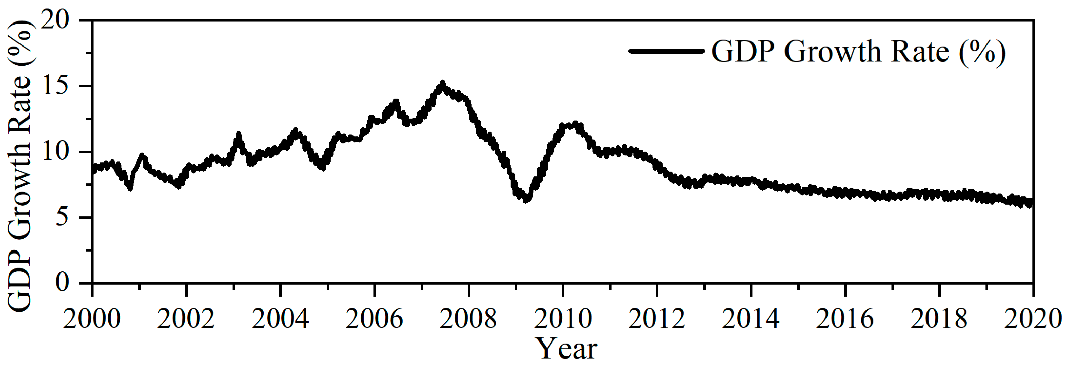
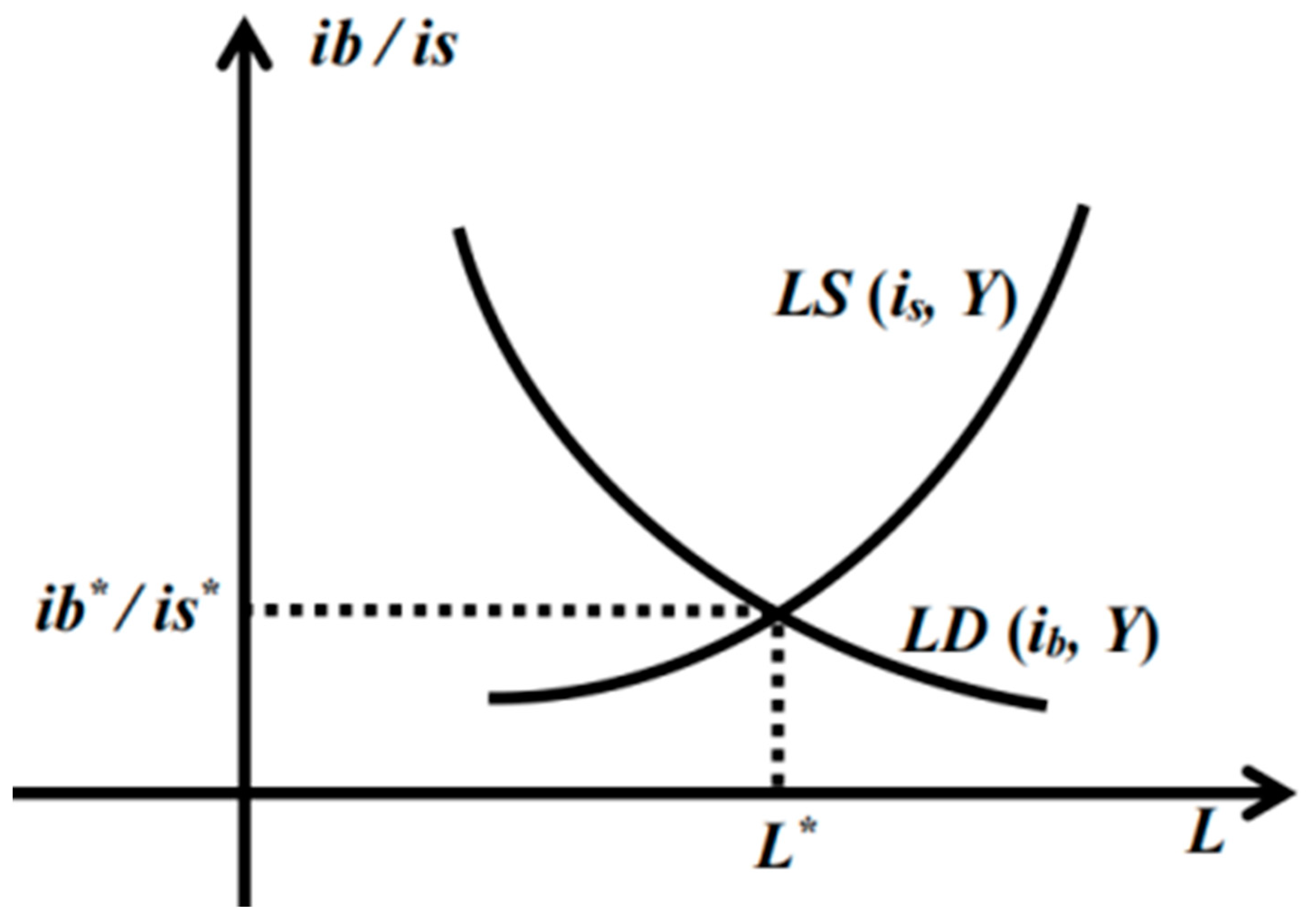
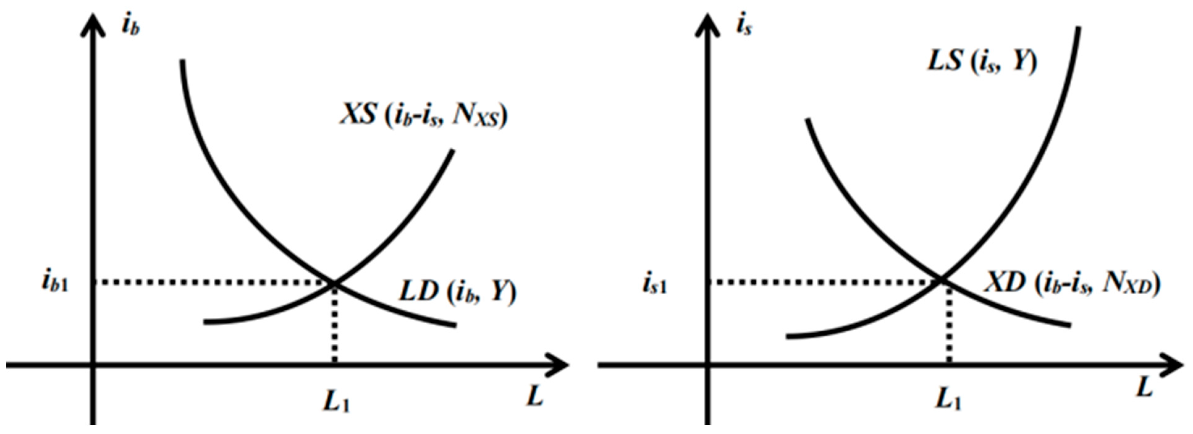
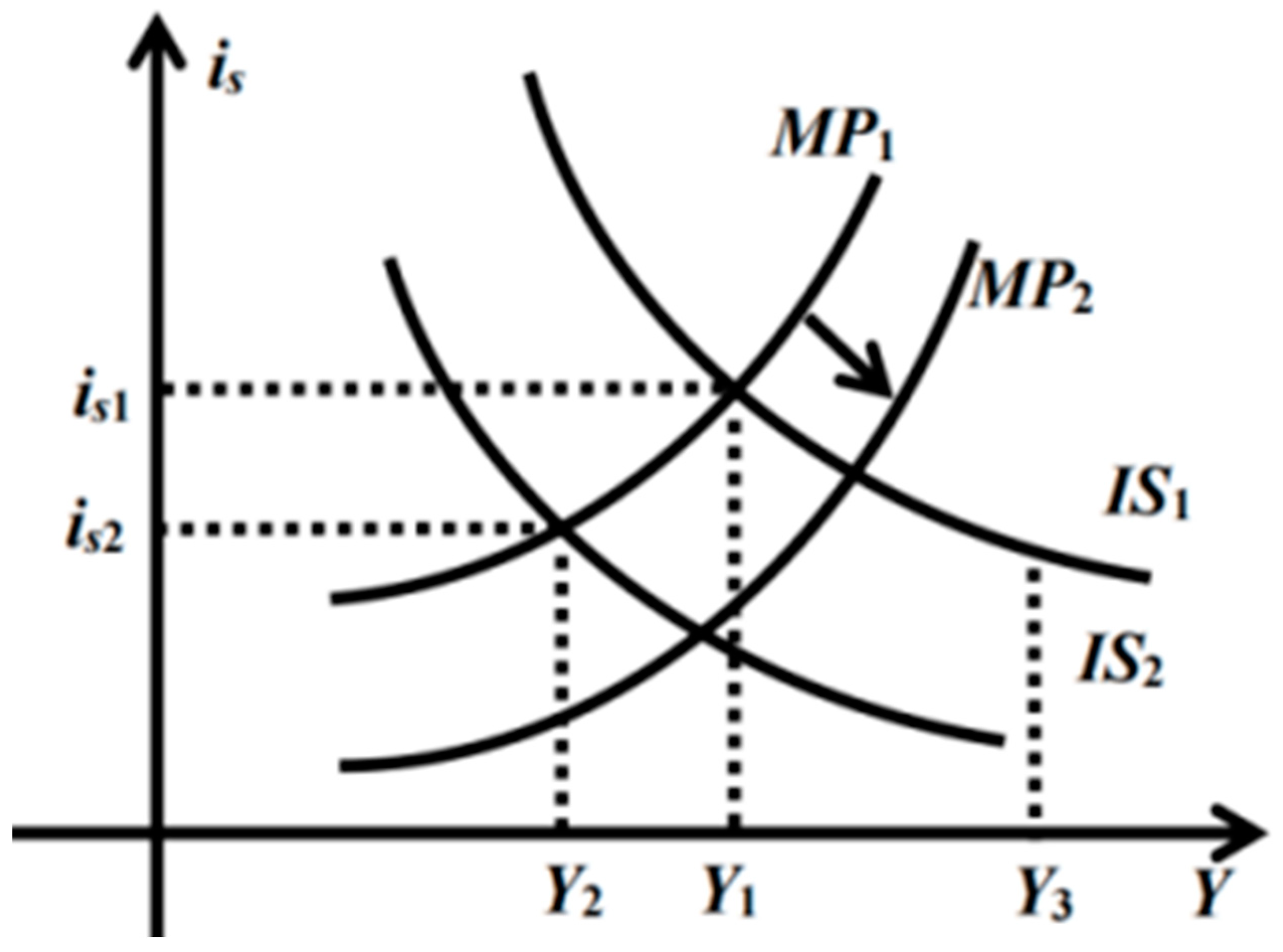
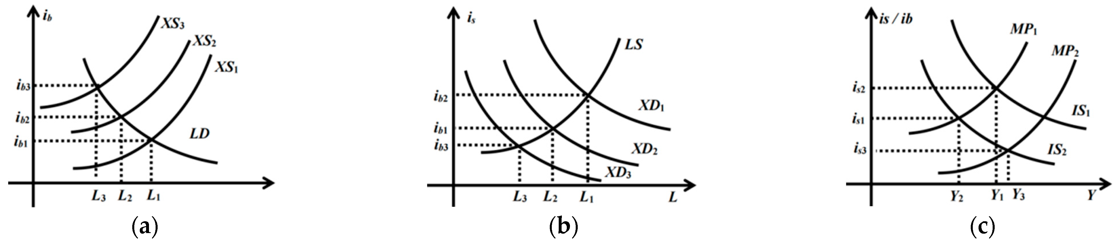
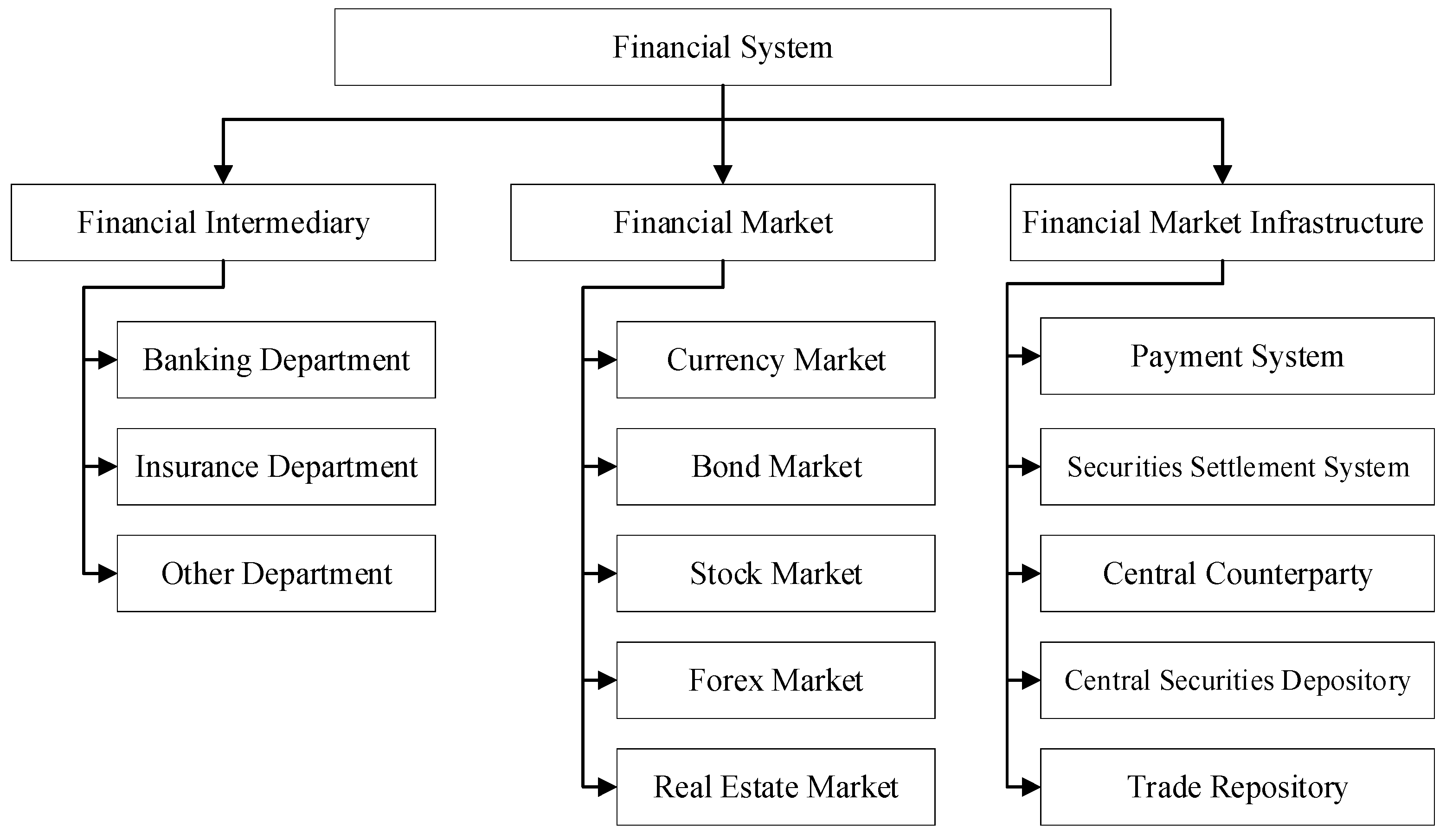
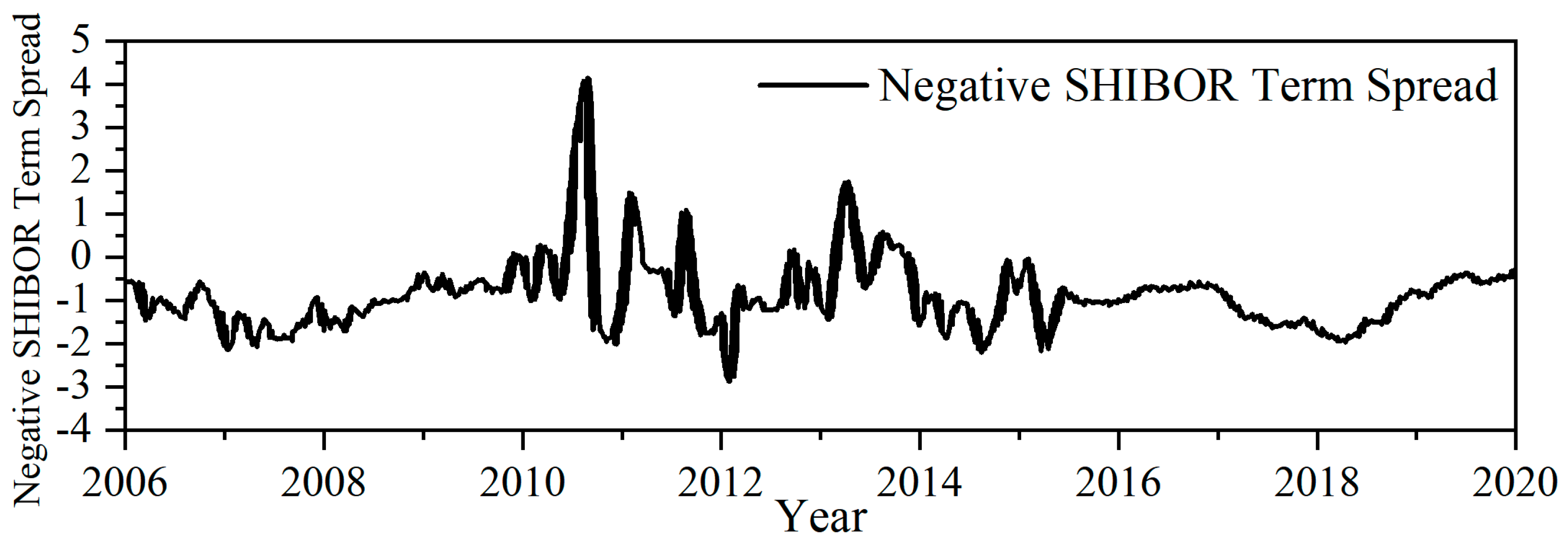
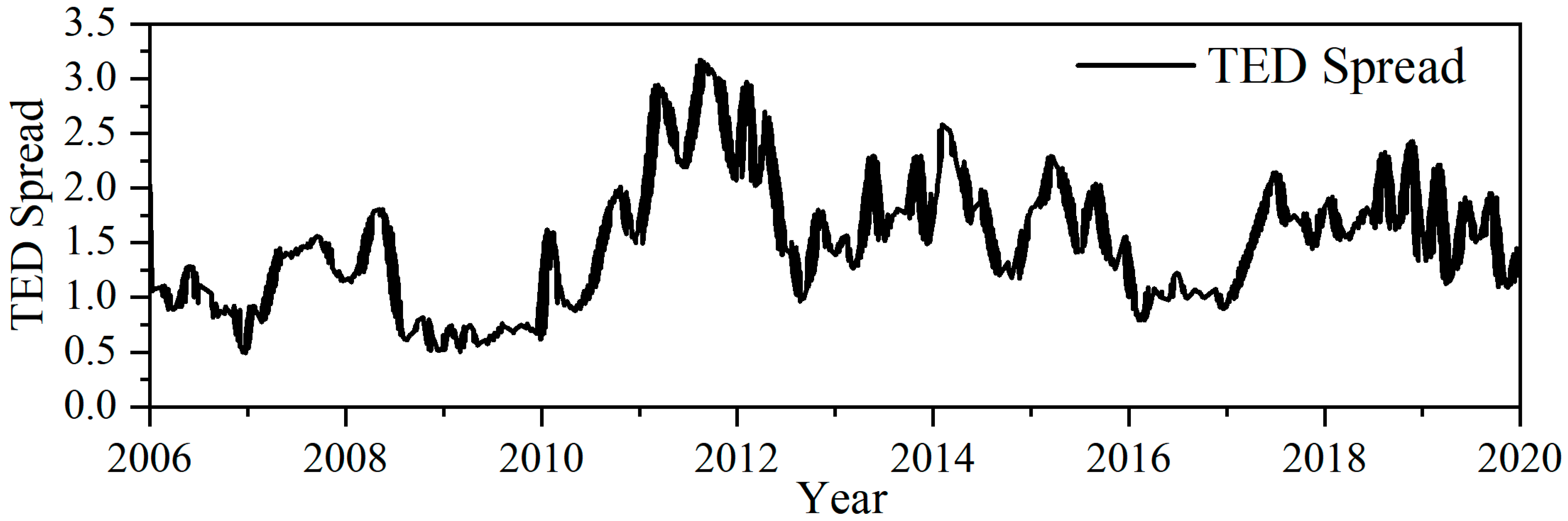
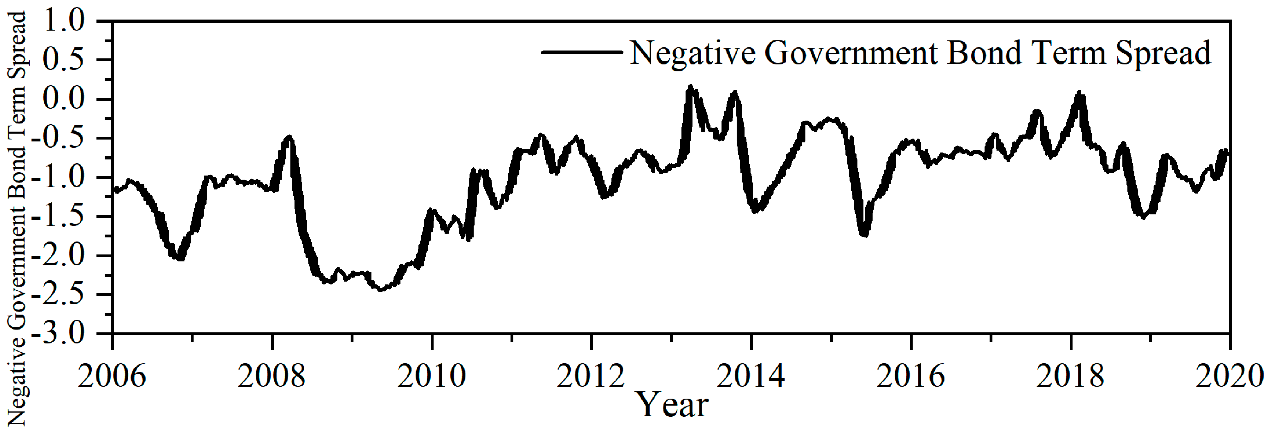
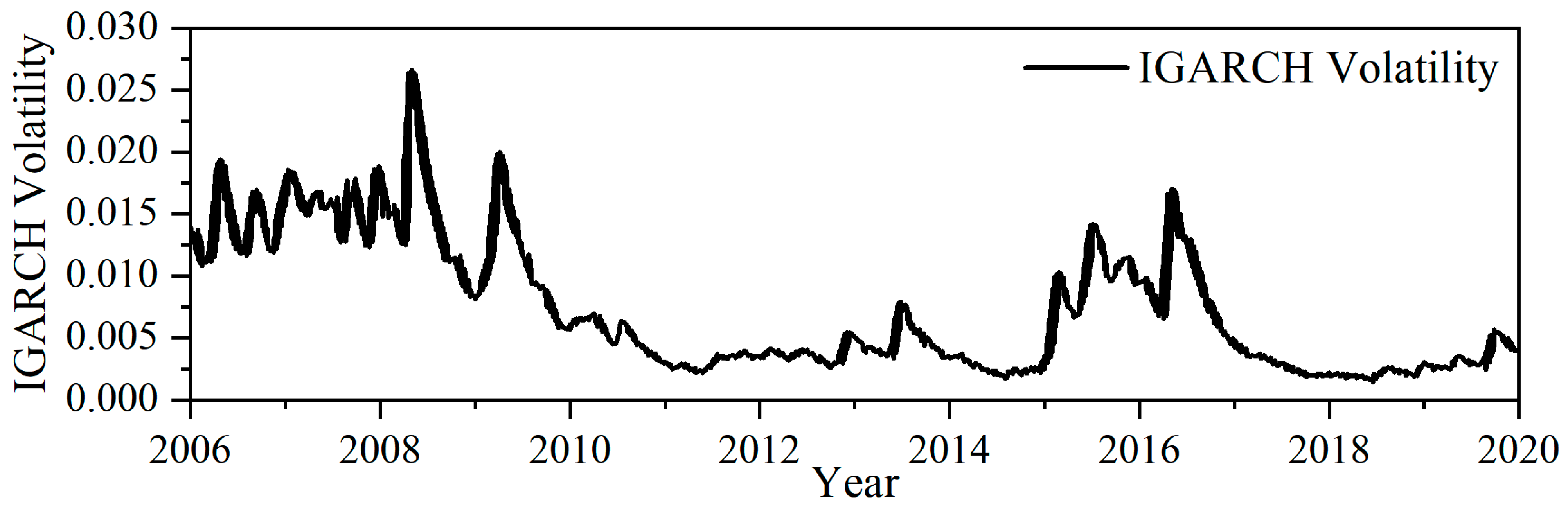
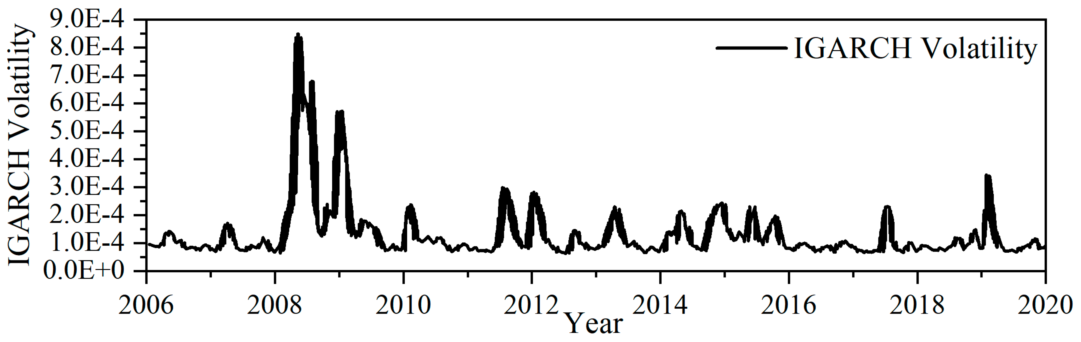
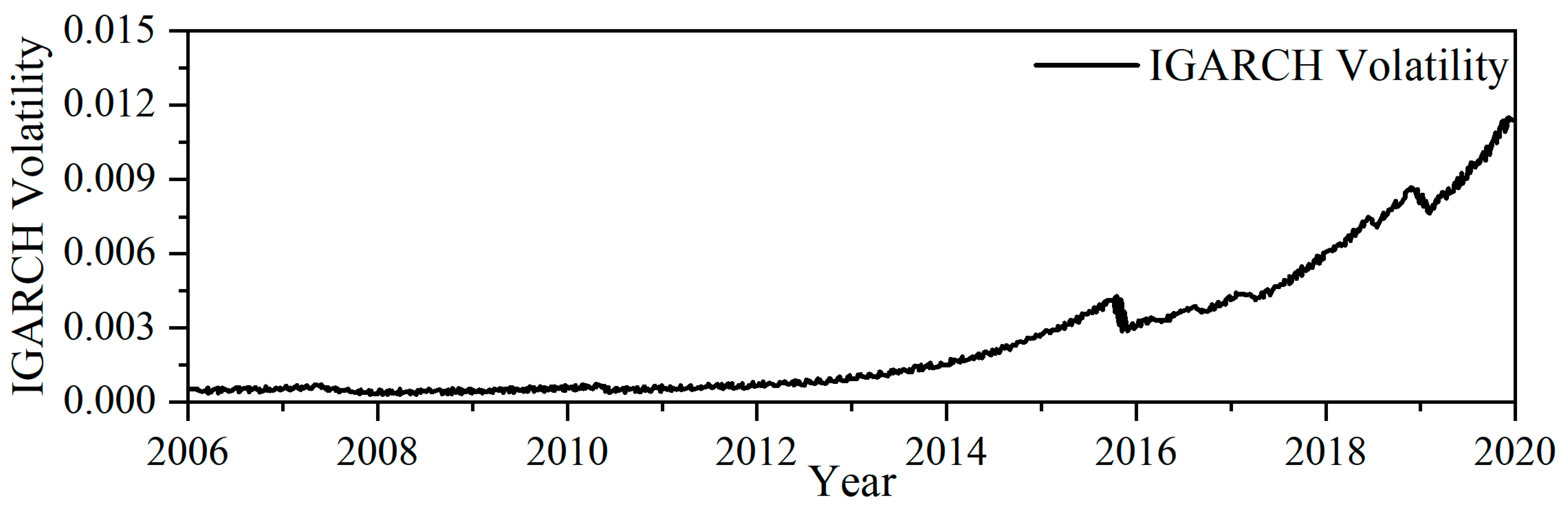
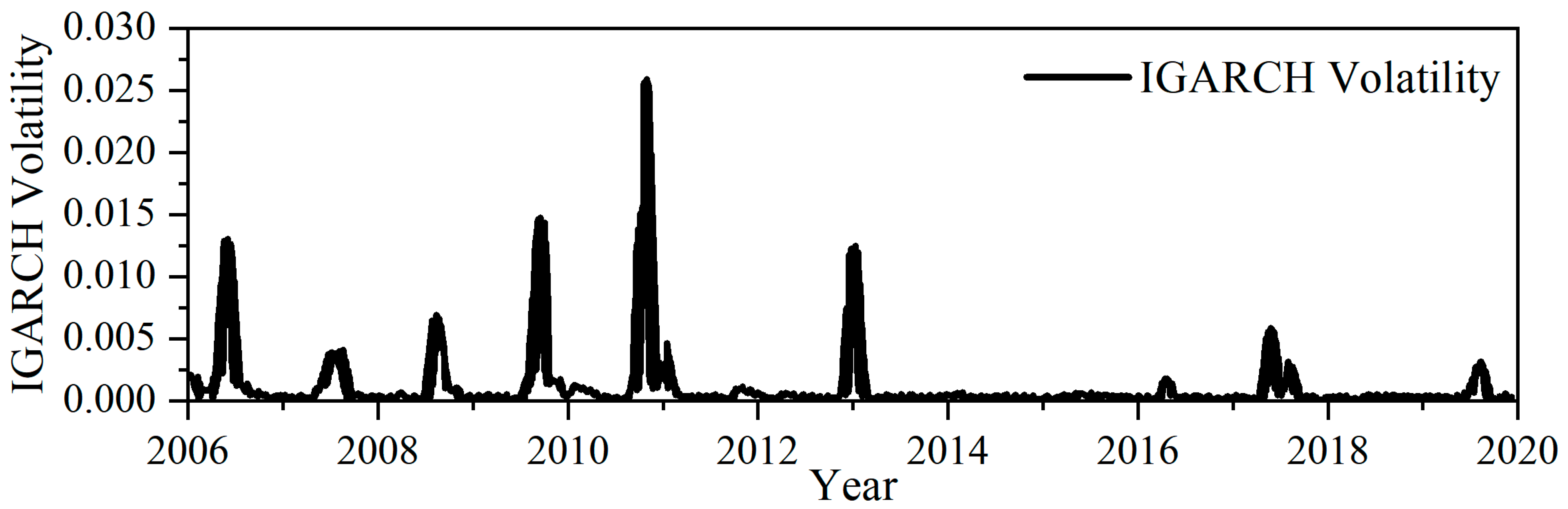
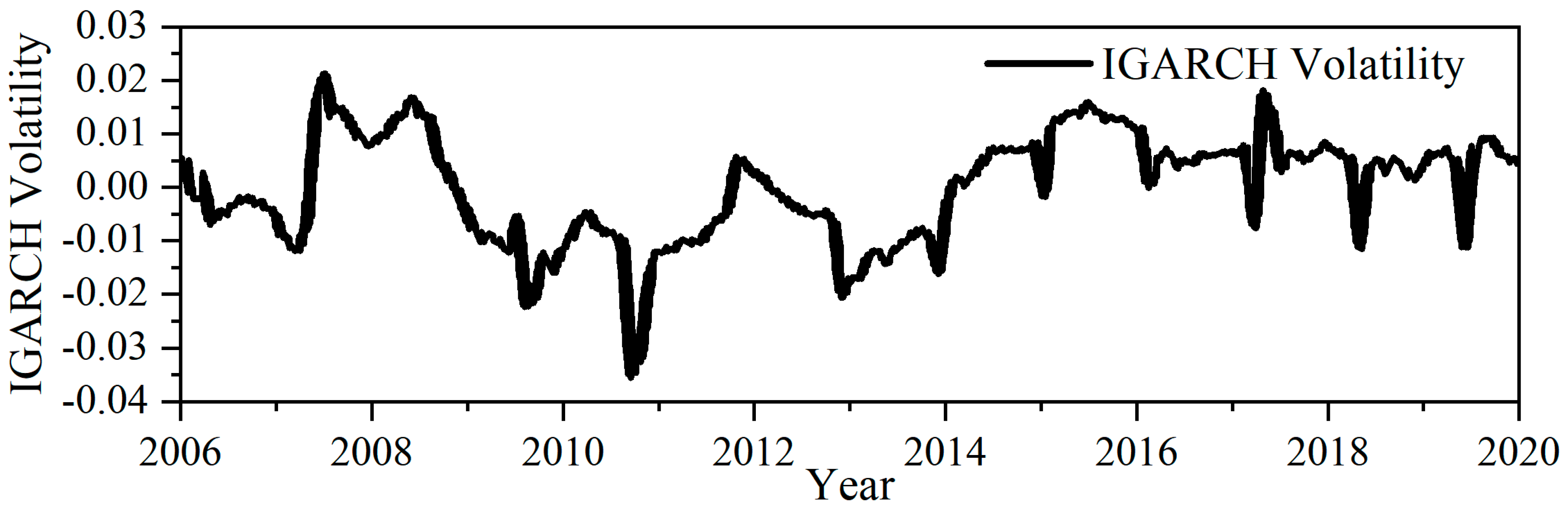
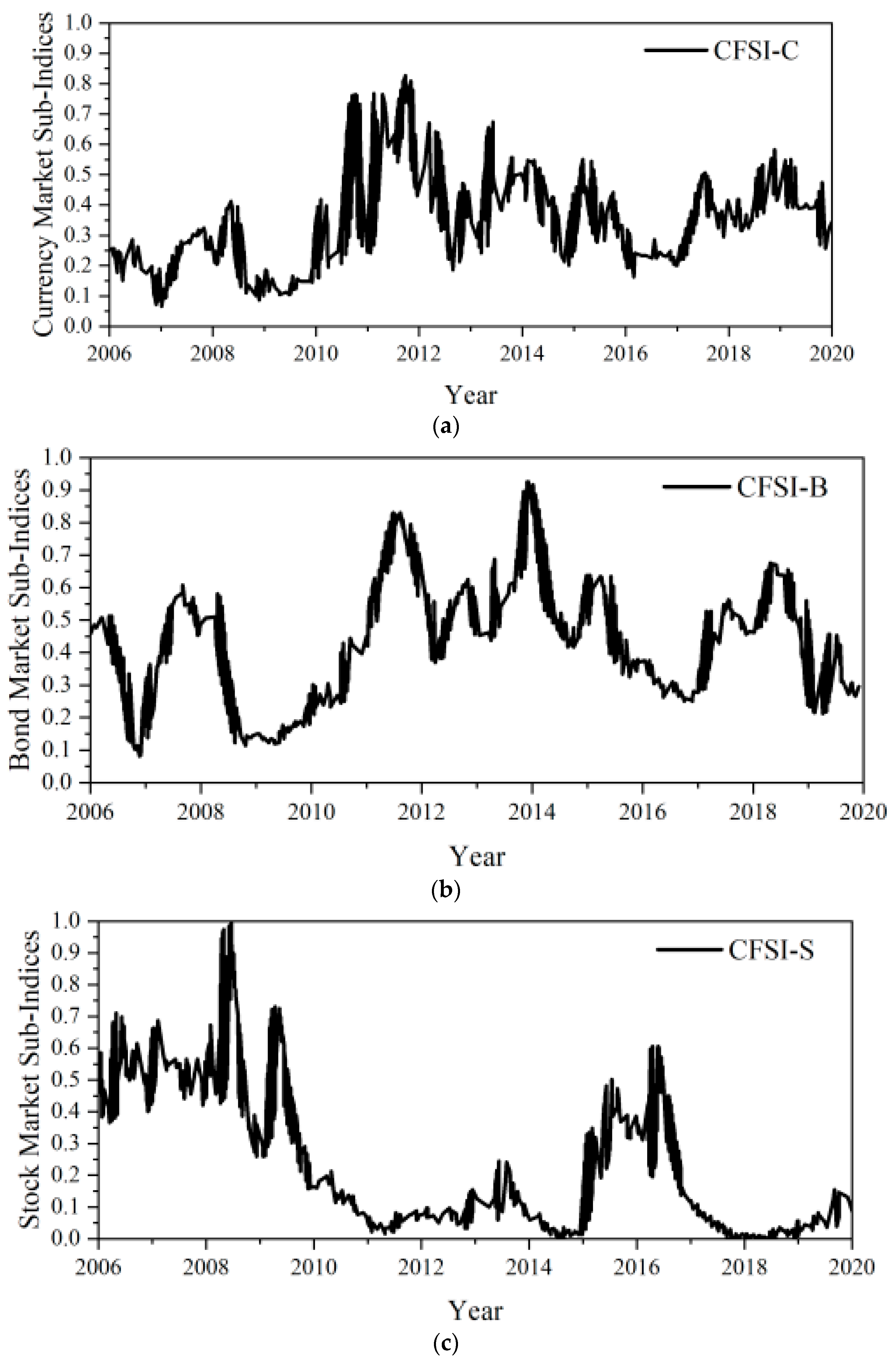
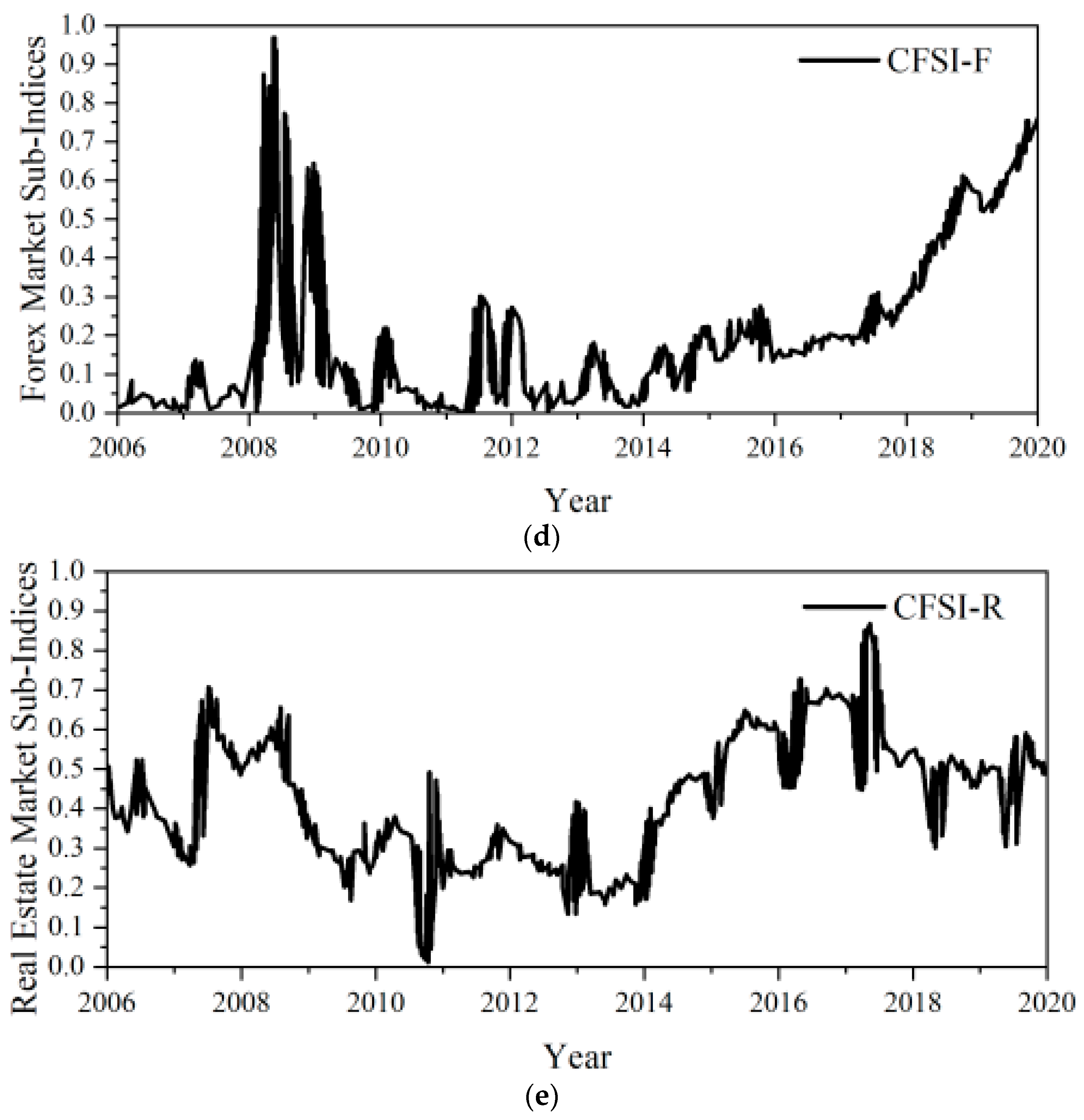
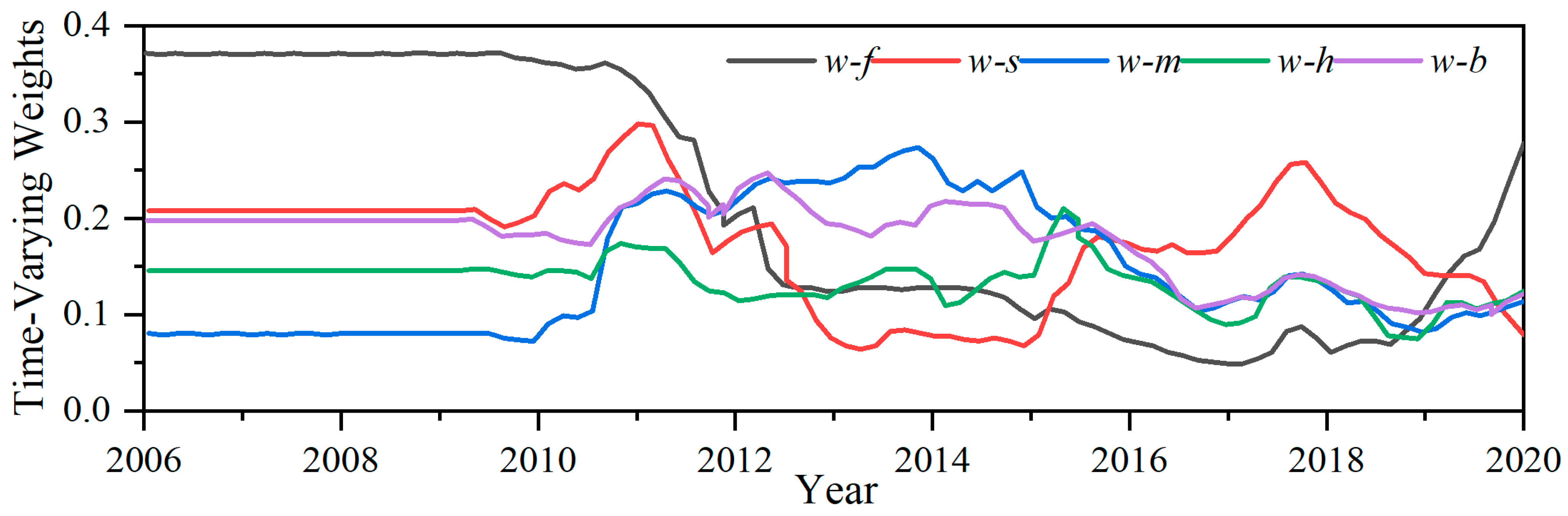
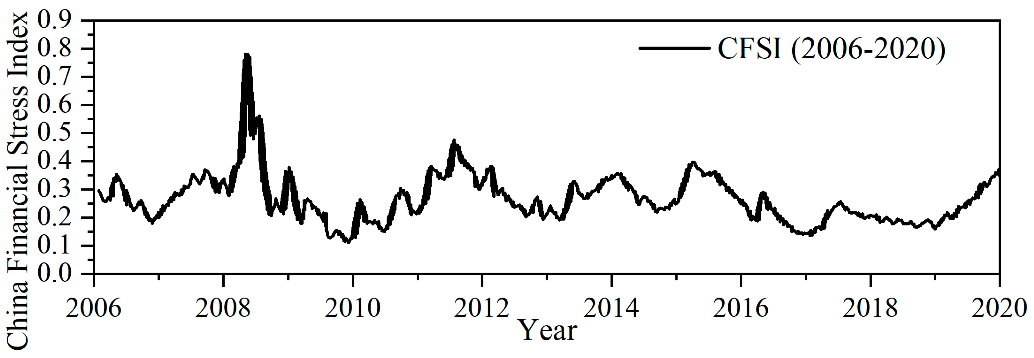
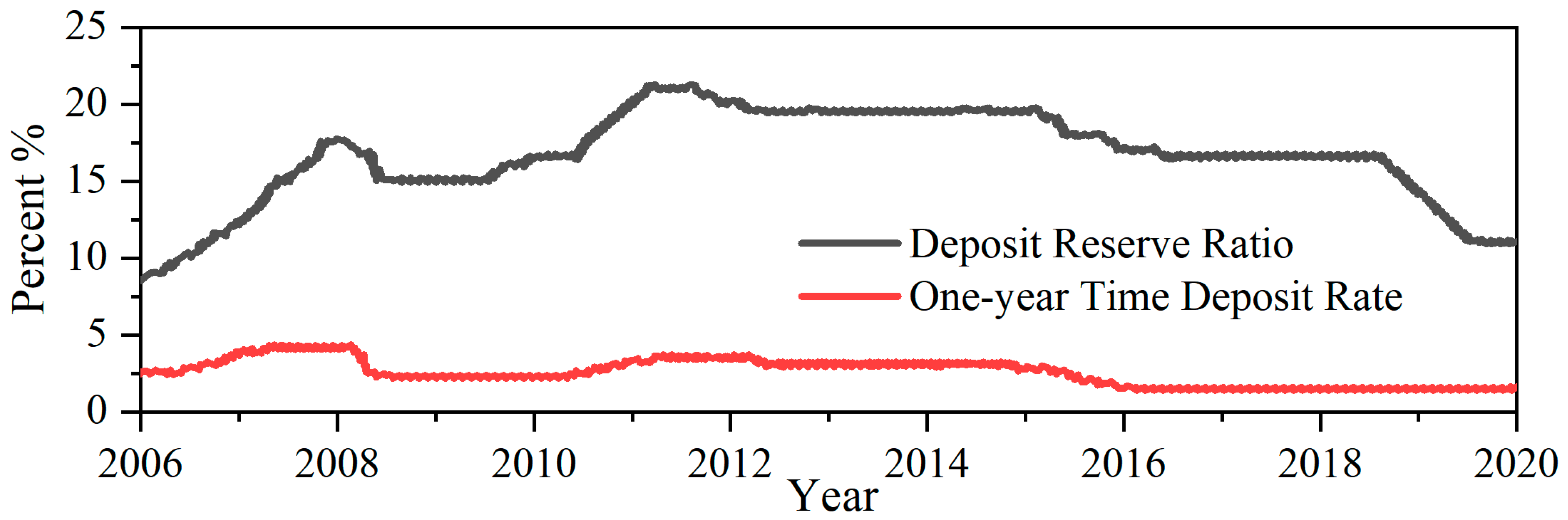
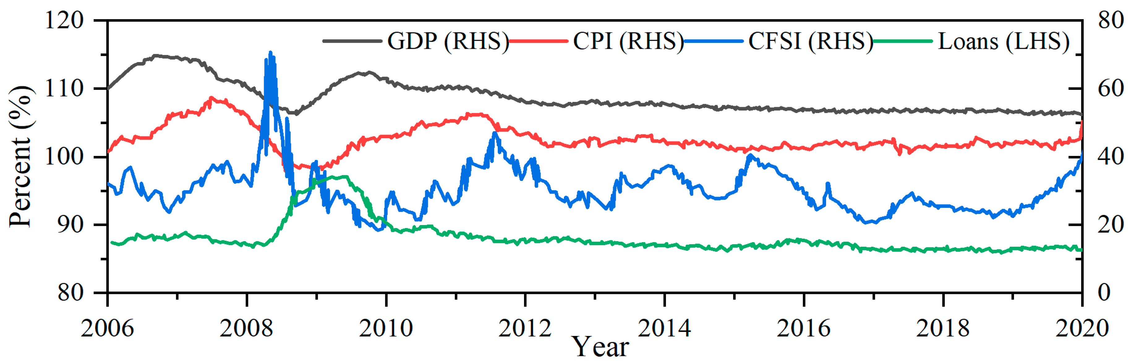
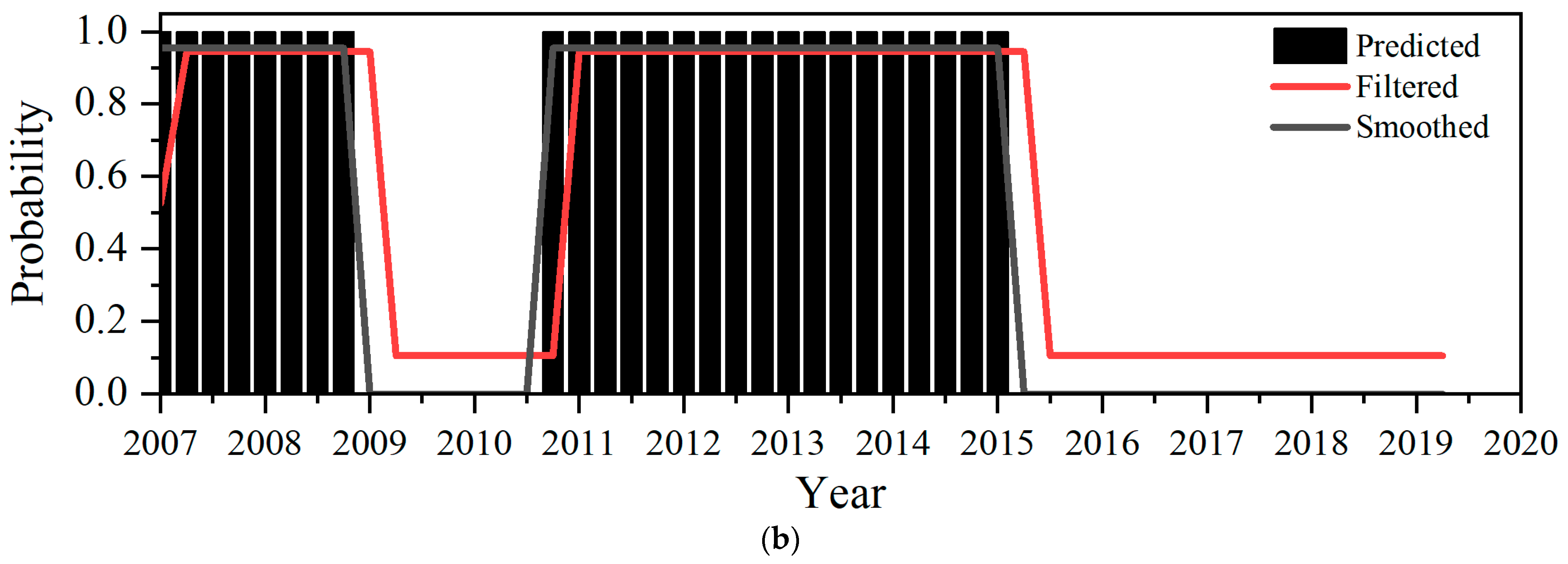
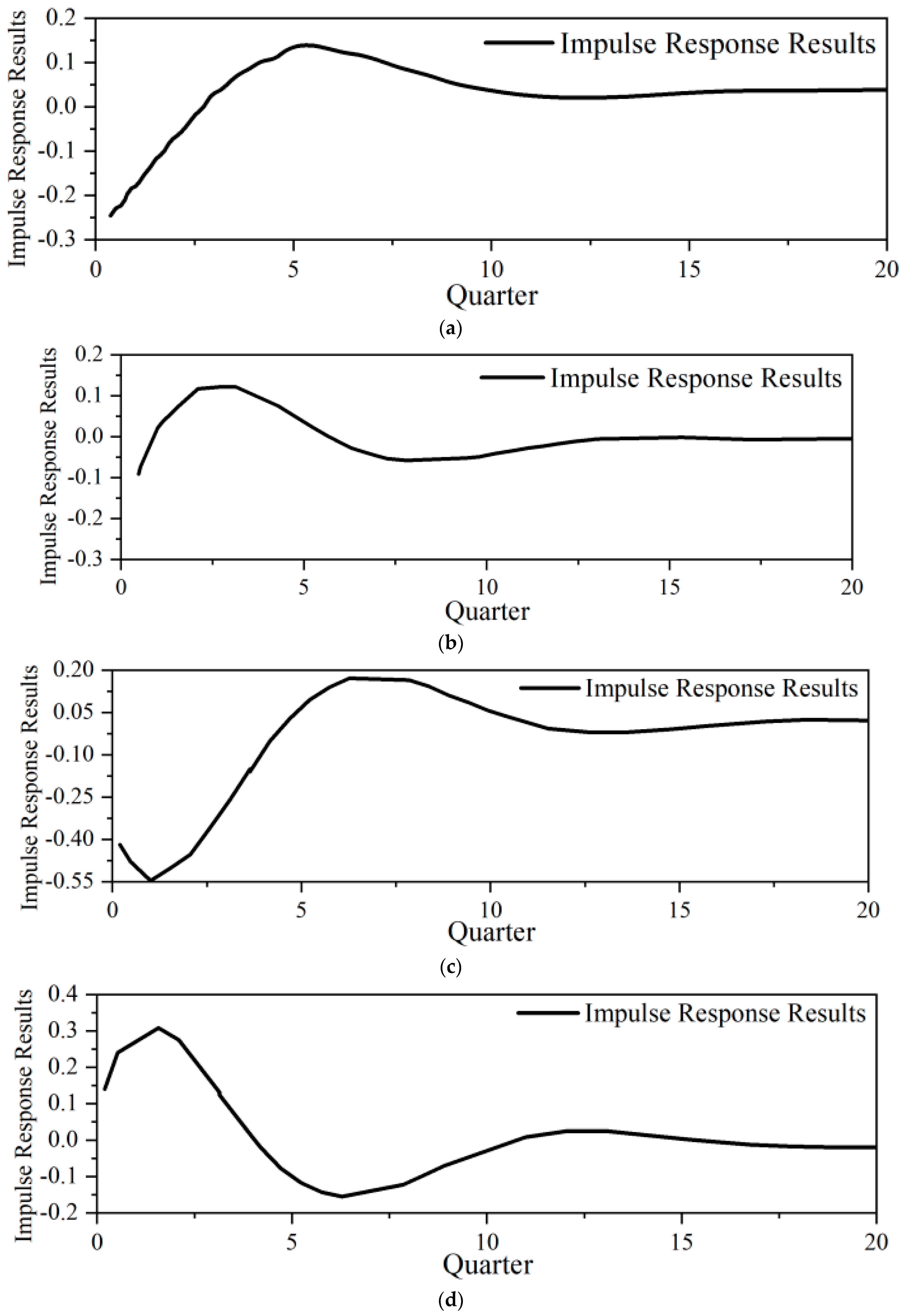
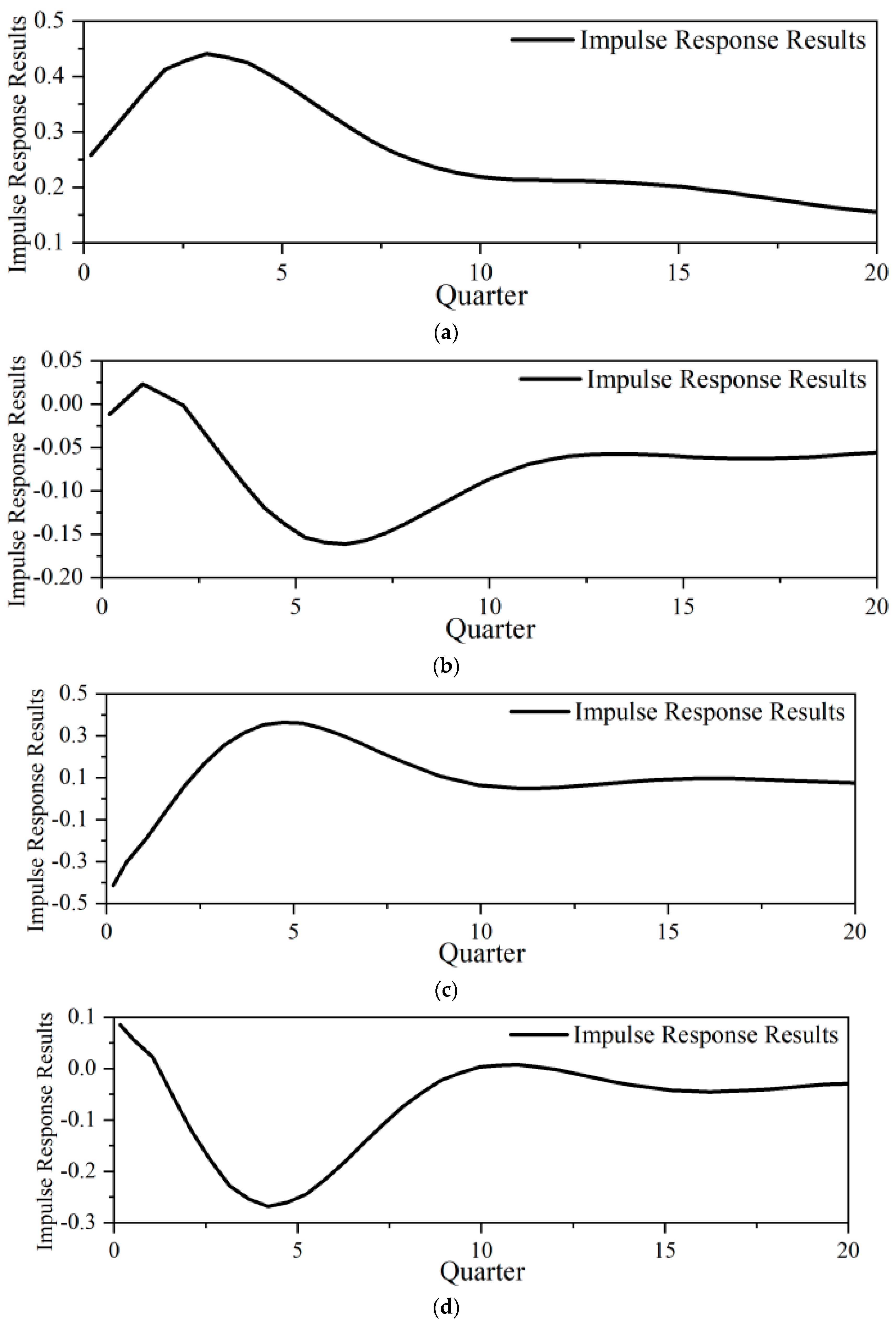
| Variable Name | Calculation Method | Influence Direction | |
|---|---|---|---|
| Currency market | SHIBOR term spread (M1) | The difference between 1-year period and 7-day SHIBOR | Negative |
| Spread between interbank offered rate and Treasury bond yield (M2) | The spread between the 3-month interbank offered rate and the 3-month Treasury bond maturity yield | Positive | |
| Bond market | Treasury bond maturity spread (B1) | The term spread between the 10-year Treasury bond and the 3-month Treasury bond yield to maturity | Negative |
| Spread between corporate bonds and government bonds (B2) | The difference between the yield to maturity of the 1-year AAA corporate bonds and the 1-year Treasury bonds | Positive | |
| Stock market | Stock price volatility (S1) | IGARCH volatility of the Shanghai Composite | Positive |
| Forex market | Real effective exchange rate volatility (F1) | IGARCH volatility of the real effective exchange rate | Positive |
| Exchange rate fluctuations (F2) | IGARCH volatility of RMB to USD | Positive | |
| Real estate market | House price volatility (H1) | IGARCH volatility of commodity housing sales prices | Positive |
| House price overvaluation level (H3) | Regression residuals of per capita disposable income and interest rates on real estate prices | Positive |
Table 2.
Variable selection and description.
| Variable Selection | Variable Description | Data Sources | |
|---|---|---|---|
| Monetary policy variables | Real money supply (rM2_gro) | Year-on-year growth rate of M2 excluding price factors | CEIC |
| Real short-term rate (rR007) | R007 excluding price factors | CEIC | |
| Real economic variables | Actual output (rGDP_gro) | Year-on-year growth rate of real GDP | CEIC |
| Inflation (CPI) | CPI year-on-year growth rate | CEIC | |
| Systemic risk level | China Financial Stress Index (CFSI) | ||
Table 3.
Variable ADF test results.
| Variable Name | T Statistic | p-Value |
|---|---|---|
| rGDP_gro | −4.900567 *** | 0.0012 |
| CPI | −4.250878 *** | 0.0014 |
| CFSI | −3.183057 ** | 0.0271 |
| rR007 | −3.327355 ** | 0.0211 |
| rM2_gro | −4.655218 *** | 0.0027 |
NOTE: “**” and “***” represent rejections of the null hypothesis at the 5% and 1% significance levels, respectively.
Table 4.
MS-VAR model form.
| Variable Mean | Variable Intercept | ||
|---|---|---|---|
| Aj Constant | Constant Variance | Markov-Switching Mean Vector Auto-Regressive Model (MSM-VAR) | Markov-Switching Intercept Vector Auto-Regressive Model (MSI-VAR) |
| Variable Variance | Markov-Switching Mean Heteroskedastic Vector Auto-Regressive Model (MSMH-VAR) | Markov-Switching Intercept Heteroskedastic Vector Auto-Regressive Model (MSIH-VAR) | |
| Aj Variable | Constant Variance | Markov-Switching Mean Autoregressive Coefficient Vector Auto-Regressive Model (MSMA-VAR) | Markov-Switching Intercept Autoregressive Coefficient Vector Auto-Regressive Model (MSIA-VAR) |
| Variable Variance | Markov-Switching Mean Autoregressive Coefficient Heteroskedastic Vector Auto-Regressive Model (MSMAH-VAR) | Markov-Switching Intercept Autoregressive Coefficient Heteroskedastic Vector Auto-Regressive Model (MSIAH-VAR) |
NOTE: Aj represents the vector autoregressive parameter matrix.
Table 5.
Model form selection basis.
| Model Form | Log Likelihood | AIC | HQ | SC |
|---|---|---|---|---|
| MSM(2)-VAR(1) | −85.499 | 5.6122 | 6.3739 | 7.6198 |
| MSMA(2)-VAR(1) | −351.0524 | 17.4715 | 18.5994 | 20.4444 |
| MSMH(2)-VAR(1) | −65.7095 * | 5.4167 * | 6.3981 * | 8.0035 * |
| MSMAH(2)-VAR(1) | −351.0524 | 18.0838 | 19.4314 | 21.6358 |
| MSI(2)-VAR(1) | −86.8419 | 5.667 | 6.4287 | 7.6747 |
| MSIA(2)-VAR(1) | −145.574 | 10.0234 | 11.4882 | 13.8843 |
| MSIH(2)-VAR(1) | −69.9882 | 5.5914 | 6.5728 | 8.1781 |
NOTE: “*” represents the selected model form.
Table 6.
Zone conversion probability matrix.
| Conversion Probability | Zone 1 | Zone 2 |
|---|---|---|
| Zone 1 | 0.9565 | 0.0435 |
| Zone 2 | 0.0769 | 0.9231 |
Table 7.
Zone estimated duration.
| Sample | Frequency | Duration | |
|---|---|---|---|
| Zone 1 | 24.0 | 0.6389 | 23.00 |
| Zone 2 | 25.0 | 0.3611 | 13.00 |
Disclaimer/Publisher’s Note: The statements, opinions and data contained in all publications are solely those of the individual author(s) and contributor(s) and not of MDPI and/or the editor(s). MDPI and/or the editor(s) disclaim responsibility for any injury to people or property resulting from any ideas, methods, instructions or products referred to in the content. |
© 2023 by the authors. Licensee MDPI, Basel, Switzerland. This article is an open access article distributed under the terms and conditions of the Creative Commons Attribution (CC BY) license (https://creativecommons.org/licenses/by/4.0/).
Share and Cite
MDPI and ACS Style
Dong, H.; Zheng, Y.; Li, N. Analysis of Systemic Risk Scenarios and Stabilization Effect of Monetary Policy under the COVID-19 Shock and Pharmaceutical Economic Recession. Sustainability 2023, 15, 880. https://doi.org/10.3390/su15010880
AMA Style
Dong H, Zheng Y, Li N. Analysis of Systemic Risk Scenarios and Stabilization Effect of Monetary Policy under the COVID-19 Shock and Pharmaceutical Economic Recession. Sustainability. 2023; 15(1):880. https://doi.org/10.3390/su15010880
Chicago/Turabian StyleDong, Hao, Yingrong Zheng, and Na Li. 2023. "Analysis of Systemic Risk Scenarios and Stabilization Effect of Monetary Policy under the COVID-19 Shock and Pharmaceutical Economic Recession" Sustainability 15, no. 1: 880. https://doi.org/10.3390/su15010880
Note that from the first issue of 2016, this journal uses article numbers instead of page numbers. See further details here.