
A hybrid of artificial neural network, exponential smoothing, and ARIMA models for COVID-19 time series forecasting
Abstract
The Auto Regressive Integrated Moving Average (ARIMA) model seems not to easily capture the nonlinear patterns exhibited by the 2019 novel coronavirus (COVID-19) in terms of daily confirmed cases. As a result, Artificial Neural Network (ANN) and Error, Trend, and Seasonality (ETS) modeling have been successfully applied to resolve problems with nonlinear estimation. Our research suggests that it would be ideal to use a single model of ETS or ARIMA for COVID-19 time series forecasting rather than a complicated Hybrid model that combines several models. We compare the forecasting performance of these models using real, worldwide, daily COVID-19 data for the period between January 22, 2020 till June 19, and June 20 till January 2, 2021 which marks two stages, each stage indicating the first and the second wave respectively. We discuss various forecasting approaches and the criteria for choosing the best forecasting technique. The best forecasting model selected was compared using the forecasting assessment criterion known as Mean Absolute Error (MAE). The empirical results show that the ETS and ARIMA models outperform the ANN and Hybrid models. The main finding from the ETS and ARIMA models analysis indicate that the magnitude of the increase in total confirmed cases over time is declining and the percentage change in the death rate is also on the decline. Our results shows that the chosen forecaste models are consistent during the first and second wave of of the pandemic. These forecasts are encouraging as the world struggles to contain the spread of COVID-19. This may be the result of the social distancing measures mandated by governments worldwide.
1.Introduction
The 2019 novel coronavirus (COVID-19) pandemic has been recognized as a global threat that is having a significant negative impact on all spheres of life, worldwide. It is a rapidly evolving emergency situation and its effects are being felt all over the world as citizens of many countries have been restricted by ‘stay at home’ orders and government-mandated social distancing measures to prevent the spread of the virus. Stock markets are crashing with prices on a down swing, mental health issues are on the rise as people go into isolation, and unemployment is surging as most industries lay off employees whose jobs must be performed on site.
In this paper, we aim to forecast total confirmed cases and death rates of COVID-19 using a hybrid model to forecast the spread of COVID-19 around the world for the next two weeks using currently available data. The forecast of confirmed cases is presented alongside the death rate to discover what should be expected in the coming days as well as to determine the best forecasting method. The relative reliability of our forecasting model cannot be overemphasized as the models for the spread of the virus can be best fitted with a combination of linear and nonlinear models. To improve the overall forecasting performance of this COVID-19 model, a hybrid model – which is a combination of a linear stochastic model, the autoregressive integrated moving average (ARIMA) model, and the nonlinear artificial neural network (ANN) and Error, Trend, and Seasonality (ETS) models – is used. Evidence from previous studies suggests that the hybrid model performs better than the linear or nonlinear models. For example, using a standardized precipitation index series, the hybrid model as well as individual stochastic and ANN models were applied to forecast drought in India and the hybrid model was found to have the greatest accuracy (Mishra et al., 2007).
The ANN model has received a great deal of attention over the last 20 years. It is one of the most powerful tools for pattern classification due to its nonlinear and non-parametric adaptive-learning properties. Many studies have been conducted that have compared ANNs with other traditional techniques (see, e.g., Safi, 2013; Valipour et al., 2012; and White & Safi, 2016), among many others. White and Safi (2016) showed that when compared to the ARIMA model, the ANN model performed well when its linking function was nonlinear. However, when its linking function was linear, the ARIMA model outperformed the ANN model. This is not surprising since the ARIMA model was designed specifically for this situation.
Several studies are being conducted using a variety of models to predict the potential evolution of the COVID-19 pandemic. These models are based on various assumptions and their associated analyses are likely subject to bias. Benvenuto et al. (2020) performed an ARIMA model prediction on the Johns Hopkins epidemiological data to predict epidemiological trends in the prevalence and incidence of COVID-2019; however, it is only reliable if we assume that the data follow only a linear pattern. In a different light, Remuzzi and Remuzzi (2020), Liu et al. (2020), and Zhao et al. (2020) used an exponential growth model to explain the spread of severe acute respiratory syndrome and COVID-19; however, this forecast is reliable only if the trends follow a strictly exponential pattern. Therefore, our proposed hybrid forecasting model is a blend of linear and nonlinear models that combines the ARIMA, ANN, and ETS models to more accurately account for the linear and nonlinear patterns in the data.
2.Data description and measures of forecasting accuracy
2.1Description of the datasets
There are currently 85,040,066 confirmed cases and 1,844,920 deaths from the coronavirus COVID-19 outbreak as of January 03, 2021, 10:37 GMT.
We consider total confirmed cases as of close of business on January 22, 2020 through June 19, 2020. In addition, we considered the data for the outcomes of all closed cases, which resulted in death, from February 2, 2020 through June 19, 2020 (Worldometer, 2020).
Figure 1 shows the total confirmed COVID-19 cases and reflects the fact that there were 1,201,483 confirmed cases of COVID-19 worldwide at the end of the day on June 19, 2020. This figure includes deaths and recovered or discharged patients (i.e., cases with an outcome). Total confirmed cases ranged between 580 and 8,750,990 with a mean of 2,418,848.85. This summary indicates that the spread of total confirmed cases varies among the various countries.
Figure 1.
Time series plot of total confirmed cases and death rate of COVID-19.
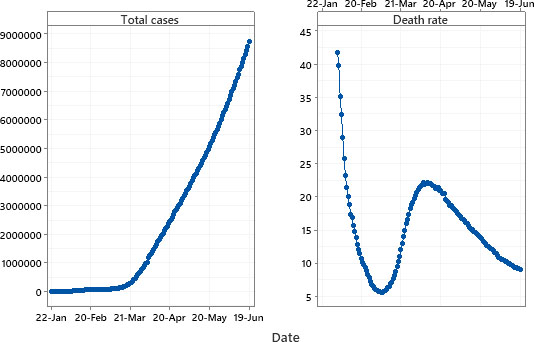
In addition, Fig. 1 shows the outcome of all closed cases (death rate) from February 2, 2020 through June 19, 2020. This figure illustrates the cumulative number of total deaths over the cumulative number of closed cases. The death rate ranges between 5.64% and 41.8% with a mean of 15.01 and a median of 14.32.
In this study, 10% of the sample size is used as the testing sample. A training sample is used for the model building, and the testing sample is used for the model validation at the end of analysis. We considered the first 135 observations as training sample for the total confirmed cases and 125 observations as training sample for the death rate of COVID-19 data.
2.2Assessment of forecasting accuracy
The accuracy of forecasts can be determined by considering how well a model performs on new data that were not used when fitting the model. Accuracy is an important issue in forecasting; therefore, researchers tend to add more and more variables to their proposed model. Safi and White (2017) considered the issue of whether a complex model does a better job than a simple one.
Many measures of forecasting accuracy have been developed and several authors have discussed the fundamental usage of these measurements and compared the accuracy of forecasting methods with univariate time series data (see, i.e., Cryer & Chan, 2008; Hyndman & Athanasopoulos, 2018; Wei, 2006). The best forecasting models selected will be compared using three different forecasting accuracy measuring criteria: mean absolute error (MAE), the root mean squared error (RMSE), and mean absolute percentage error (MAPE).
Definition 1. Suppose
(1)
Definition 2. The RMSE is defined as:
(2)
The RMSE has been popular, largely because of its theoretical relevance in statistical modeling (Hyndman et al., 2002). However, this measure is more sensitive to outliers than the MAE, which has led some authors (e.g., see Armstrong, 2001) to recommend using other measures of forecasting accuracy. The MAE is preferable in cases of the existence of outliers. Using the MAE or RMSE is recommended when comparing forecasting methods on a single data set. This means, the MAE and RMSE should be used if all forecasts are measured on the same scale.
Definition 3. The MAPE is defined as:
(3)
The MAPE presents the forecast error in terms of percentage and hence it is scale invariant and unit-free (Lyhagen et al., 2015). The MAPE is a simple average of absolute percentage errors. It is recommended to use MAPE when comparing the accuracy of the same or different methods on different time series data with different scales, unless the data contain zeros or small values (Hyndman & Koehler, 2006).
The evaluation criterion for these measures of forecasting accuracy is that the smaller the value obtained, the better the model’s forecasting ability (McKenzie, 2011).
Definition 4. The efficiency of the proposed forecasting method relative to that of the benchmark method in terms of the RMSE,
(4)
where RMSEp and RMSEb represent the RMSE from the proposed and the benchmark methods, respectively. Usually the benchmark method is the most naïve method (Hyndman, 2006). A ratio of less than one indicates that the forecasting performance of the proposed method is more efficient than the benchmark method and if
3.Forecasting models
3.1The ARIMA model
The general ARIMA
(5)
where
(6)
and
(7)
The best ARIMA model is chosen according to its Akaike information criterion (AIC), AICc, or BIC value.
3.2The exponential smoothing model
The exponential smoothing method has been in use since the 1950s and is still the most popular forecasting method used in business and industry. The field of exponential smoothing has undergone a substantial evolution over the past 10 years.
Let
(8)
(9)
where
3.3The ANN model
The nnetar function is used to fit neural networks. This function is described as a feed-forward neural network with a single hidden layer and lagged inputs for forecasting univariate time series. The nnetar function fits a neural network autoregressive
3.4The hybrid model
The hybrid model fits multiple individual model specifications to enable the easy creation of ensemble forecasts. The hybrid model consists of a combination of three models: the ARIMA, the exponential smoothing, and the ANN models. Looking at a time series composed of autocorrelated linear and nonlinear components, we have:
(10)
Fitting
(11)
The error term consists of nonlinear relationships with previous errors. The nonlinear relationships can be modeled from the past residuals as follows:
(12)
Then, using an ANN model to predict
(13)
These models were built using hybrid Model command in the forecast Hybrid package. This package fits multiple models and combines them using either equal weights or weights based on in-sample errors. There are six models: ARIMA, exponential smoothing, theta, neural network autoregression (NNAR), seasonal and trend decomposition, and the trigonometric seasonal
4.Empirical results
This section presents the empirical results of the models used to forecast the total confirmed cases and the recovery or death rate using four different approaches; the ARIMA, ETS, ANN models, and the hybrid combination of the three models. The forecasting results are presented in the following sub-sections.
4.1Test for normality
We carried out the Anderson-Darling (AD) normality test to determine if the residuals after approximation for the four models followed a normal distribution (Thode, 2002).
For the total confirmed cases’ residuals of COVID-19 data, normality test yielded the following AD values: 8.8922, 7.5803, 6.22, and 9.645, with corresponding
For the death rates residuals’, the normality test yielded the following AD values: 4.976, 0.535, 2.368, and 1.029, with corresponding
Since the data are not normally distributed (without loss of generality), to compare the performance of the models through the two datasets, we used the forecasting accuracy measure, the MAE, over the forecasting period for each model. The smaller values of MAE indicate higher forecasting accuracy. Therefore, the ratios of the MAE of the hybrid model to those of the ARIMA, ETS, and ANN models were calculated for analysis.
4.2Relative efficiencies of the empirical results
Table 1 lists the complete empirical results for the ratios of the hybrid model’s RMSE, MAE, and MAPE of residuals after approximation to those of the ARIMA, ETS, and ANN models for total confirmed cases and the death rate. Since the data are not normally distributed, we discuss these empirical results based on the ratios of the hybrid model’s MAE to those of the ARIMA, ETS, and ANN models.
Table 1
Ratios of the RMSE, MAE, and MAPE for the hybrid to the ARIMA, ETS, and ANN models
| Dataset | Statistic | Hybrid/ARIMA | Hybrid/ETS | Hybrid/ANN |
|---|---|---|---|---|
| Total confirmed cases | RMSE | 1.5142 | 1.5700 | 0.5865 |
| MAE | 1.5089 | 1.5638 | 0.5890 | |
| MAPE | 1.5070 | 1.5611 | 0.5897 | |
| Death rate | RMSE | 1.1804 | 1.1068 | 0.7950 |
| MAE | 1.1682 | 1.1417 | 0.7593 | |
| MAPE | 1.1699 | 1.1384 | 0.7629 |
Table 2
Forecast in total confirmed cases and death rate for the full data
| Date | Total cases | Death rate |
|---|---|---|
| 20-Jun | 8,901,699 | 9 |
| 21-Jun | 9,055,284 | 8.92 |
| 22-Jun | 9,208,869 | 8.84 |
| 23-Jun | 9,362,454 | 8.76 |
| 24-Jun | 9,516,039 | 8.69 |
| 25-Jun | 9,669,624 | 8.63 |
| 26-Jun | 9,823,209 | 8.57 |
| 27-Jun | 9,976,794 | 8.52 |
| 28-Jun | 10,130,379 | 8.47 |
| 29-Jun | 10,283,964 | 8.42 |
| 30-Jun | 10,437,549 | 8.38 |
| 1-Jul | 10,591,134 | 8.34 |
| 2-Jul | 10,744,719 | 8.3 |
| 3-Jul | 10,898,304 | 8.27 |
| 4-Jul | 11,051,889 | 8.24 |
4.3Total confirmed cases data
Applying the ANN model with average of 10,000 networks, each of which is a 1-25-1 network, with 76 weights and estimated noise variance of 1.33e+08. This indicates that 25 networks were trained and that their predictions were averaged. For the hybrid model, the weights for the ARIMA, ETS, and ANN models were chosen to be equal. For the ARIMA model, the result shows that the best fit model was the ARIMA (0, 2, 1) with estimated moving average coefficient
For the exponential smoothing model, simple exponential smoothing with additive errors is fitted. The estimated values of the model smoothing parameters are
The relative efficiencies based on residuals after approximation of the hybrid model to the ARIMA, ETS, and ANN models equal
Therefore, the ETS model perfroms more efficient as compared to ARIMA, and was superior than the ANN and Hybrid models for total confirmed cases of COVID-19 data. However, as a second choice in this case, we could use the ARIMA model since it is almost as efficient as the ETS model, keeping in mind that it is not a perfect substitute.
4.4Death rate data
The ANN model with an average of 10,000 networks, each of which was a 1-25-1 network, with 76 weights and estimated noise variance of 0.2494. This indicates that 25 networks were trained and that their predictions were averaged. For the hybrid model, the weights for the ARIMA, ETS, and ANN models were chosen to be equal. For the ARIMA model, the result shows that the best fit model is ARIMA (2,0,2) with zero mean and estimated noise variance equaling 0.09114 (with AIC
Figure 2.
Forecasts and Actual values in total confirmed cases and death rate.
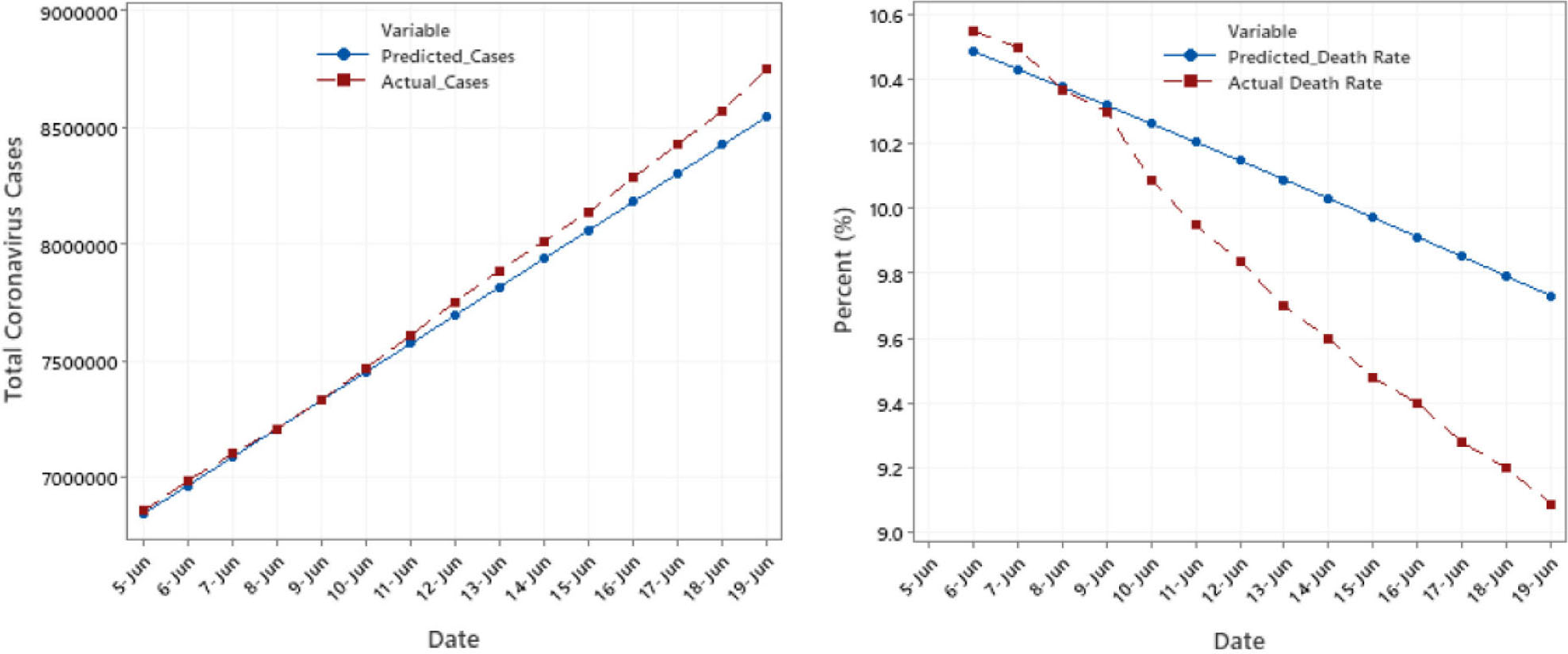
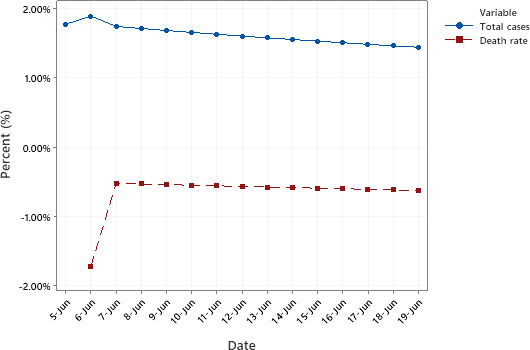
Figure 3.
Time Series Plot of percentage change* from the forecast in total confirmed cases and death rate. *The percentage change is
The relative efficiencies based on residuals after approximation of the hybrid to the ARIMA, ETS, and ANN models equal
Therefore, the hybrid model performed poorly as compared to the ARIMA and ETS models and was more efficient than the ANN model for forecasting the total confirmed cases and the death rate of COVID-19 data. Therefore, the ANN model is not the best choice for forecasting COVID-19 death rates, and ARIMA outperforms the other models.
Table 3
Actual and forecast in total confirmed cases and death rate
| Total cases | Death rate | |||
|---|---|---|---|---|
| Date | Actudal | Forecast | Actudal | Forecast |
| 20-Jun | 8,884,614 | 8,901,699 | 8.99 | 9 |
| 21-Jun | 9,016,161 | 9,055,284 | 8.88 | 8.92 |
| 22-Jun | 9,156,852 | 9,208,869 | 8.8 | 8.84 |
| 23-Jun | 9,321,853 | 9,362,454 | 8.7 | 8.76 |
| 24-Jun | 9,496,903 | 9,516,039 | 8.57 | 8.69 |
| 25-Jun | 9,678,539 | 9,669,624 | 8.53 | 8.63 |
| 26-Jun | 9,874,597 | 9,823,209 | 8.41 | 8.57 |
| 27-Jun | 10,053,182 | 9,976,794 | 8.34 | 8.52 |
| 28-Jun | 10,218,466 | 10,130,379 | 8.27 | 8.47 |
| 29-Jun | 10,381,866 | 10,283,964 | 8.18 | 8.42 |
| 30-Jun | 10,558,291 | 10,437,549 | 8.09 | 8.38 |
| 1-Jul | 10,758,053 | 10,591,134 | 7.99 | 8.34 |
| 2-Jul | 10,968,830 | 10,744,719 | 7.83 | 8.3 |
| 3-Jul | 11,184,378 | 10,898,304 | 7.75 | 8.27 |
| 4-Jul | 11,381,197 | 11,051,889 | 7.66 | 8.24 |
Figure 4.
Actual data in total confirmed cases and death rate.
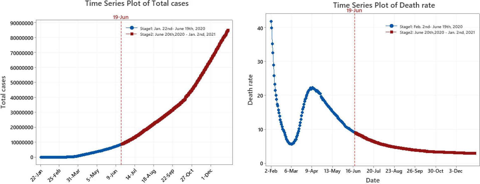
Figure 5.
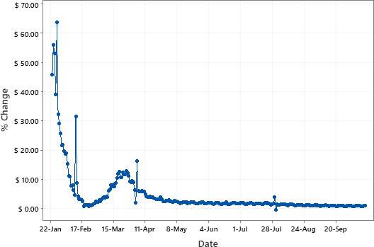
Time Series Plot of percentage change in total confirmed cases.
5.Model forecasting
The forecast for total comfirmed cases and death rates using the ETS and ARIMA respectively is compared with the actual values as shown in Fig. 2. We could observe from this Fig that the predicted values are close to the actual values. This substantiates the valid use of the models.
In Fig. 3, we show the forecasts and percentage changes in total confirmed cases and the death rate calculated using the ETS and ARIMA models, respectively, to forecast the next 14 days (June 4–June 19). The prediction intervals are preserved from the individual component models and use the most extreme values from each individual model, producing conservative estimates for the combination’s performance.
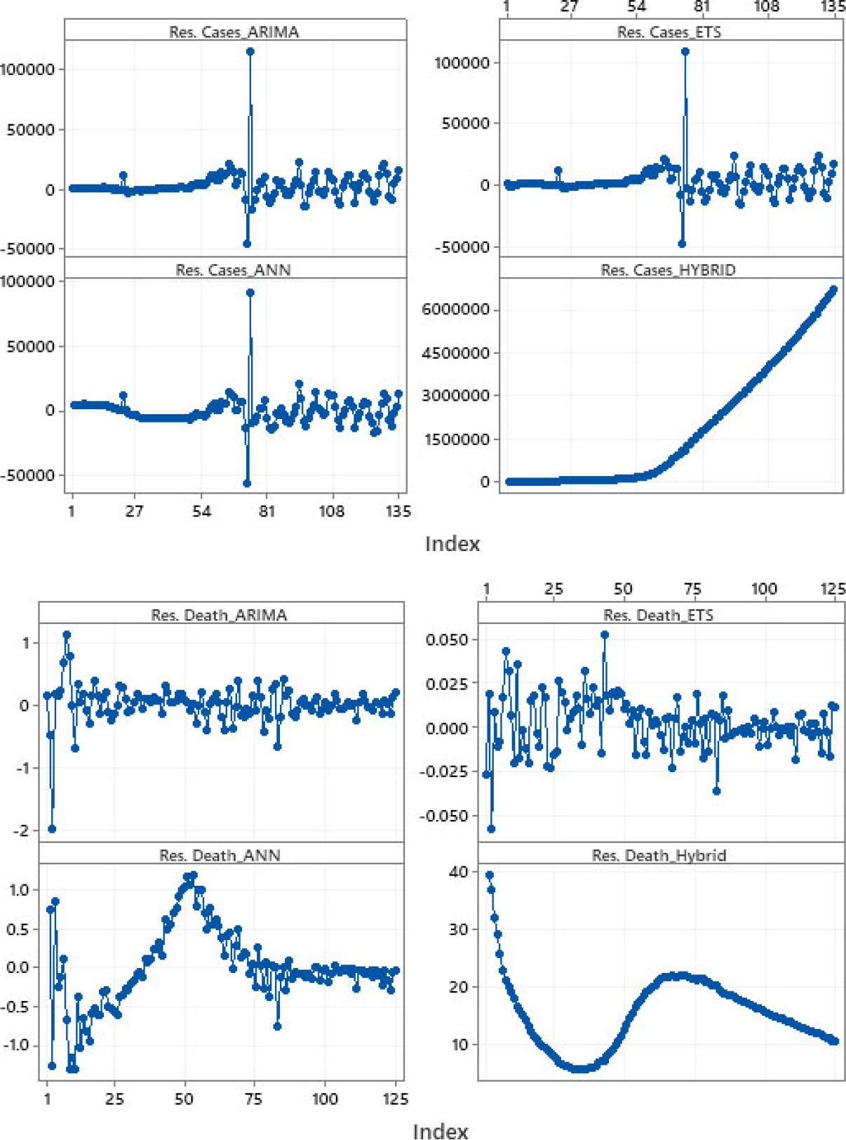
Figure 6.
Time series plot for residuals of the total confirmed cases and the death rate.
After feeding the model with data from June 4–June 19, and repeating the procedure, we show the forecasts in total confirmed cases and the death rate for the next 14 days (June 20–July 4). This is shown in Table 2.
In our forecast for June 20th till July 4th, the daily total confirmed cases is shown to be on the increase, however, this increase is at a decreasing rate. The death rate exhibit a declining trend which increases our optimism as the fight to contain the COVID-19 continues.
Table 3 shows actual and forecast numbers in total confirmed cases side by side the actual and forecast of death rate. The figure illustrates the increase in total confirmed cases of the actual data alongside the forecast value from January 20th till July 4th 2020. From the plots we observe the closeness of our forecast value to the actual value, indicating that our selected model in forecasting the total confirmed cases is relatively close to the actual values, hence, this can be reliable for policy implementation. For the death rate, the figure illustrates a decline in both the actual and forecast values and the forecast value for the death rate is closer to the actual rates. However, the chosen forcasting model which is relatively higher prepares policy makers for the worst case scenario as we go through the second wave of the pandemic.
6.First wave and suggested second wave of COVID-19
In Fig. 4, we show two different stages of the actual data of total confirmed cases and death rate for COVID-19 each separated by a partition. The total confirmed cases for the first stage which is the data used for the initial analysis and forecasts starts from January 22
Figure 5 shows the time series plot of percentage changes in total confirmed cases of COVID-19. The daily total confirmed cases is on the increase while the percentage change in total confirmed cases is declining, which indicates that the magnitude of increase over time of total cases is falling. Overall, the results shows that our chosen forecaste model is consistent in both the first and the second wave of the pandemic. This result is promising as the world enters the second wave of the spread of COVID-19.
7.Conclusions and future research
We used the hybrid model to exploit the capabilities of the ARIMA, ANN, and ETS models in time series forecasting of COVID-19 trends. Forecasting performance was compared based on the residuals for these models using the current daily data for COVID-19 around the world for forthcoming days. We further enumerated, explained, and discussed the various forecasting approaches and the criteria for choosing a forecasting technique that provides the best forecasts for total confirmed cases and the death rate for COVID-19.
The results show that the ETS and ARIMA models outperforms the ANN and Hybrid models. This is not a surprising fact as the ARIMA model is well-fitted to stationary residuals as exhibited in the sample period as shown in Fig. 6. This result adds to the growing body of literature that seeks to accurately forecast the spread of COVID-19 by combining and examining the validity of multiple models used by other researchers. We were able to establish that the use of complicated models such as ANN and Hybrid does not necessarily provide the best results. With the ETS and ARIMA models, the forecasting results indicate that there are brighter days ahead as we observe a percentage decrease in new total daily cases and a decline in the death rate percentage respectively around the world. Our findings shows that the chosen forecaste models are consistent during the first and second wave of of the pandemic. This forecast strengthens our optimism that, more people will recover from COVID-19 as the mortality rate declines.
In addition, there is more hope as many countries are racing to discover a cure as well as a vaccine that would mitigate the negative effects of COVID-19. Further research could be carried out in this area by studying a Hybrid model that combines ARIMA and ETS in contrast to the individual use of either ARIMA or ETS to forecast total cases and death rates. Also, one could examine the impact of COVID-19 on economic variables using the most appropriate forecasting techniques.
References
[1] | Armstrong, J. S. ((2001) ). Principles of forecasting: A handbook for researchers and practitioners. Springer Science & Business Media, 30: . |
[2] | Benvenuto, D., Giovanetti, M., Vassallo, L., Angeletti, S., & Ciccozzi, M. ((2020) ). Application of the ARIMA model on the COVID-2019 epidemic dataset, Data in Brief, 105340. |
[3] | Cryer, J., & Chan, K. ((2008) ). Time series analysis with applications in R. Springer, New York. |
[4] | Hyndman, R. J. ((2004) ). New in Forecast 4.0. http://robjhyndman.com/hyndsight/forecast4/. |
[5] | Hyndman, R. J., & Athanasopoulos, G. ((2018) ). Forecasting: Principles and practice. OTexts. |
[6] | Hyndman, R. J., & Koehler, A. B. ((2006) ). Another look at measures of forecast accuracy, International Journal of Forecasting, 22: , 679-688. |
[7] | Hyndman, R. J., Akram, M., & Archibald, B. C. ((2008) ). The admissible parameter space for exponential smoothing models, Annals of the Institute of Statistical Mathematics, 60: , 407-426. |
[8] | Hyndman, R. J., Koehler, A. B., Snyder, R. D., & Grose, S. ((2002) ). A state space framework for automatic forecasting using exponential smoothing methods, International Journal of Forecasting, 18: , 439-454. |
[9] | Liu, Y., Gayle, A. A., Wilder-Smith, A., & Rocklöv, J., ((2020) ). The reproductive number of COVID-19 is higher compared to SARS coronavirus, Journal of Travel Medicine. |
[10] | Lyhagen, J., Ekberg, S., & Eidestedt, R. ((2015) ). Beating the VAR: Improving Swedish GDP forecasts using error and intercept corrections, Journal of Forecasting, 34: , 354-363. |
[11] | McKenzie, J. ((2011) ). Mean absolute percentage error and bias in economic forecasting, Economics Letters, 113: , 259-262. |
[12] | Mishra, A. K., Desai, V. R., & Singh, V. ((2007) ). Drought forecasting using a hybrid stochastic and neural network model, Journal of Hydrologic Engineering, 12: , 626-638. |
[13] | Remuzzi, A., & Remuzzi, G. ((2020) ). COVID-19 and Italy: What next? The Lancet. |
[14] | Safi, S. K. ((2013) ). Artificial neural networks approach to time series forecasting for electricity consumption in Gaza strip, Artificial Neural Networks Approach to Time Series Forecasting for Electricity Consumption in Gaza Strip, 21: . |
[15] | Safi, S. K., & White, A. K. ((2017) ). Short and long-term forecasting using artificial neural networks for stock prices in Palestine: A comparative study, Electronic Journal of Applied Statistical Analysis, 10: , 14-28. |
[16] | Thode, H. C. ((2002) ). Testing for normality. CRC press. 164: . |
[17] | Valipour, M., Banihabib, M. E., & Behbahani, S. M. R. ((2012) ). Monthly inflow forecasting using autoregressive artificial neural network, Journal of Applied Sciences, 12: , 2139-2147. |
[18] | Wei, W. ((2006) ). Time Series Analysis Univariate and Multivariate Methods, Second edition, Pearson Education, Inc. |
[19] | White, A., & Safi, S. K. ((2016) ). The efficiency of artificial neural networks for forecasting in the presence of autocorrelated disturbances, The Efficiency of Artificial Neural Networks for Forecasting in the Presence of Autocorrelated Disturbances, 5: . |
[20] | Worldometer, C. C. ((2020) ). 1-22. |
[21] | Zhao, S., Musa, S. S., Fu, H., He, D., & Qin, J. ((2019) ). Simple framework for real-time forecast in a data-limited situation: The Zika virus (ZIKV) outbreaks in Brazil from 2015 to 2016 as an example, Parasites & Vectors, 12: , 344. |

