
Energy and Environmental Effects of Human Habits in Residential Buildings Due to COVID-19 Outbreak Scenarios in a Dwelling near Rome


Energy Efficiency Unit Department (DUEE), Italian National Agency for New Technologies, Energy and Sustainable Economic Development (ENEA), 00123 Rome, Italy
*
Author to whom correspondence should be addressed.
Energies 2021, 14(21), 7408; https://doi.org/10.3390/en14217408
Submission received: 29 September 2021
/
Revised: 3 November 2021
/
Accepted: 4 November 2021
/
Published: 7 November 2021
(This article belongs to the Section G: Energy and Buildings)
Abstract
:The COVID-19 pandemic and resulting containment measures have shown that energy consumption in buildings is linked to several factors, such as living habits, occupancy profiles, and heating ventilation and air conditioning (HVAC) systems. This paper addresses the influences of such factors on energy consumption in a residential building, analysing different scenarios (pre-COVID-19, lockdown, post-COVID-19), in terms of discomfort and energy needs, through the new hourly calculation method (UNI EN ISO 52016). Energy and environmental effects were studied in a real case study near Rome by varying occupancy profiles, lighting and appliance schedules, and HVAC systems. Results show that, during the heating period, the lockdown scenario led to the lowest hours of discomfort (−29% on average), but the highest in the cooling period (up to +154%, +28% on average). The same scenario led to reasonable reduction of energy needs for heating (−14%), but also highlighted a significant increase (+60%) for the cooling period. This study underlines how the pandemic has influenced the energy and environmental behaviours in buildings. Moreover, the new hourly calculation method points out the importance of analysing HVAC systems, in terms of hours of discomfort, which could provide results that are more reliable.

1. Introduction
Growing attention on energy consumption in the building sector, and efforts made to reduce it (especially in most developed countries) have led, throughout the years, to a decrease in energy intensity. Indeed, the final energy use per m2 (which is a measure for the energy intensity) has been decreasing by a yearly rate of 0.5% to 1% since 2010. However, this virtuous trend has not pair with the average annual floor area growth, which has remained around 2.5% since 2010 [1]. This means that energy efficiency measures (for new and renovated buildings) proceed slower than floor area expansion.
Because building stock retrofitting mainly concerns the building envelope and the heating, ventilation, and air conditioning (HVAC) system, these actions must be improved in order to accelerate the renovation process.
Regarding the building envelope—its improvements in energy efficiency is responsible for half of the total expenses for energy-related investments [1]. For the HVAC systems, the efforts in promoting (on an average global level) heat pumps, renewable energy systems (RES), efficient electric technologies, and district heating are struggling, in regard to substituting fossil fuel-based assets (including boilers, furnaces, and cook stoves) [1].
In addition to these strategies, to achieve energy intensity reduction of at least 2.5% per year, the sustainable development scenario (SDS) requires stricter measures, especially a shift in building management and use, since it could be misleading to address the total building consumption exclusively to the envelope or to the HVAC system characteristics.
In fact, factors influencing the energy use of a building are multiple and are clearly outlined in the literature: occupancy profiles [2,3,4,5,6], appliance schedules [7,8], and human behaviour [9,10] are involved in the final energy consumption.
In [11], a novel data-driven procedure attempted to improve building energy modelling reliability, taking into account representative occupant-related electric load profiles and yearly occupancy profiles.
In [2], four occupancy profiles and four thermal comfort strategies were implemented in a residential building model, to realistically represent occupants and their activities. Results show variability with occupancy profile (and with the number and age of occupants) as well as with the adopted control strategies, suggesting that correct assumptions and data regarding these aspects are needed for accurate building model.
The recent work by Flett et al. [3] highlights the importance of realistic occupancy models and the consequent electrical demand, by using and adapting existing datasets and probabilistic modelling methods, whilst in [4], the occupancy profiles of households allowed identifying peak load and, therefore, energy-saving margins and opportunities within the peak load shift.
In [6], a multi-storey Zero Energy Building (ZEB) building model, representative of the current real estate market, was developed. The influence of occupancy, ventilation, and shading system schedules was assessed by comparison with the “reference case” (referred to customized/tailored profiles), showing the relevance of such aspects in the design phase, especially in low-energy consuming buildings.
Even appliance use influences the building’s total consumption, but home energy management system profitability depends on the number of inhabitants and on CO2 emissions and pricing models [7].
These considerations also apply to the tertiary sector. In [5], simulation of human behaviour in office building were carried out, showing that persistent changes in habits can lead to relevant energy savings (up to 28% in energy use). In [8], the occupancy patterns in office spaces were used to obtain, by a decision tree, the occupancy schedule usable in building energy modelling.
Besides the evidences from the literature, the relevance of occupancy profiles, schedules, and habits inside our homes were experienced by everyone during the pandemic, as living habits changed [12,13] and, in turn, the energy consumption [14,15] and corresponding billing.
Indeed, pandemic containment measures adopted in many countries introduced movement restrictions, forbade people from exiting their homes (with few exceptions) [16], and forced people to stay at home for several hours, changing the way dwellings were used, lived, and experienced, with reflections on energy consumption [17,18,19].
The pandemic has disrupted living habits and changed work places [20], forcing people to experience new ways of working and networking, causing socioeconomic drawbacks [21], as well as some positive implications for the environment (e.g., CO2 reduction due to mobility reduction) [22].
Homes have suddenly become places for living, sleeping, cooking, working, studying, and keeping fit, with the possibility (and need) of using appliances at any time. Thus, total energy consumption has changed, affecting energy consumption at a large scale such as in districts or municipalities [23,24,25,26], or counties [27,28], and at a small scale (e.g., homes), as also proven by questionnaire surveys [29] and monitoring [30].
In particular, in [30], the authors found that lockdown measures influenced electric and hot water consumption and use, when the most intensive lockdown measures were applied, impacting consumer energy bills and how energy utilities might have been solicited during the pandemic.
Finally, an interesting study [31] underlined the strict correlation between occupancy and, on the one hand, HVAC system energy consumption, and on the other hand, the transmission of COVID-19, depending on the number and distribution of the occupants. Even if the researchers analysed a university building, some considerations can be extended to all building typologies, including housing. For example, it is necessary to maximize the ventilation rate and to correctly schedule the users’ presence in order to reduce infection risk. At the same time, it is useful to decrease the ventilation rate up to the allowed rate, when possible, and to promote climate adaptive occupant distribution, to decrease energy consumption.
This work aims to quantify how the changes in living habits (i.e., occupancy profiles and the related lighting and appliance schedules), due to containment measures and prolonged lockdowns, alter the building energy consumption
The building model of a reference case was developed and validated by adopting the new energy calculation method provided by UNI EN ISO 52016 [32], which seems to be very promising in reliability of energy performance, although only few applications can be found in the literature [33,34,35,36,37,38].
These two points (influence of human habits and use of the new calculation method to assess energy consumption) concur to the novelty of the study, since this kind of work has not been carried out in the literature.
Three different scenarios, which refer to different occupant habits (that reflect pre- and post-pandemic real occupancy profiles of owner dwellings) were also implemented. Moreover, two HVAC systems equipping the dwelling were modelled, to assess the implications of the heating system use on the total consumption.
Indeed, considering that many buildings are undergoing refurbishments and substitutions of gas-fired boilers with heat pumps, it is worth considering and assessing the implications of this kind of HVAC system. This, also in the case of human habit permanent change, is likely to occur, considering that some restrictions and limitations are ongoing.
Comparisons were carried out, in terms of discomfort hours, energy need, and CO2 emissions.
Therefore, this paper aims to: (i) analyse the effects of human habits (defined according to pre- and post-COVID-19 pandemic period), occupancy profiles, and HVAC systems in regard to the energy consumption of buildings; (ii) adopt a new energy calculation procedure, under the rules of UNI EN ISO 52016; (iii) analyse the three considered scenarios in terms of discomfort hours and energy needs.
The novelties of the paper are: (i) the application of the new hourly energy calculation method provided by UNI EN ISO 52016, for the energy consumptions assessment of a real case study near Rome (validated with its energy carriers bills); (ii) thermal energy analyses of HVAC systems, by correlating energy needs with the hours of discomfort; (iii) thermal-energy analyses carried out by adopting three different scenarios linked to the pre- and post-COVID-19 pandemic period.
Our research questions are: (i) how many discomfort hours could there be in the different occupancy scenarios? (ii) How much does an occupancy profile change a building’s final energy consumption? (iii) How much do human habits (and new schedules, due to the pandemic) influence a building’s CO2 emissions?
2. Materials and Methods
The comparison between hours of discomfort, energy consumption, and environmental impacts related to different human habits, pre- and post-COVID-19 pandemic, requires a methodology that considers different scenarios, changing the significant parameters related to these aspects.
The assumption was to select three human behaviours, representative of the changes in lifestyle that occurred in this pandemic. The choice was made, taking into account two particular aspects—work and social life. Regarding work, the Italian government adopted legislative prescription to avoid infection diffusion, promoting “smart working” at home and determining great changes in the lifestyles of workers. In fact, if during the pre-COVID-19 period, staying in the office was substantially diffused, after that, many public and private companies adopted remote solutions to guarantee the safety and health of their employees. At the same time, this action brought some indirect consequences, such as savings, in terms of management costs, and a better quality of life for commuters, leading to the adoption of this kind of work even when the pandemic situation had improved. The second aspect to be considered is the change in sociability, due to the closures of all meeting places (gyms, theatres, cinemas, etc.) and the reduction of outside activities that improved home hobbies and chores.
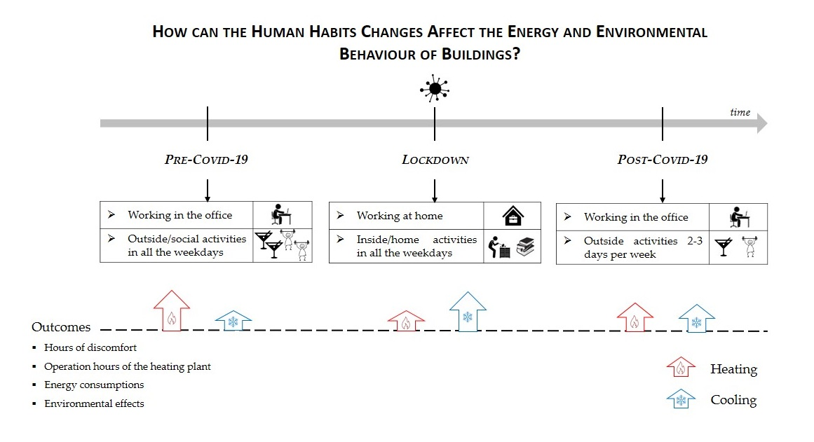
This study makes comparisons among the pre-COVID-19 lifestyle, lockdown (i.e., during the COVID-19 pandemic), and post-COVID-19 (Figure 1). All three lifestyles were defined according to occupant habits. Particularly, before the pandemic (corresponding to the pre-COVID-19 lifestyle of the user [39]), active behaviour, characterized by outside activities on all days throughout the week, was found. After the pandemic (corresponding to the post-COVID-19 lifestyle of the user), custom (social and outside) activities that took place two–three days throughout the week was, instead “taken over”. People worked in their offices in both cases. The lockdown lifestyle (during the pandemic) was associated with working at home and predominately inside activities, to avoid infection.
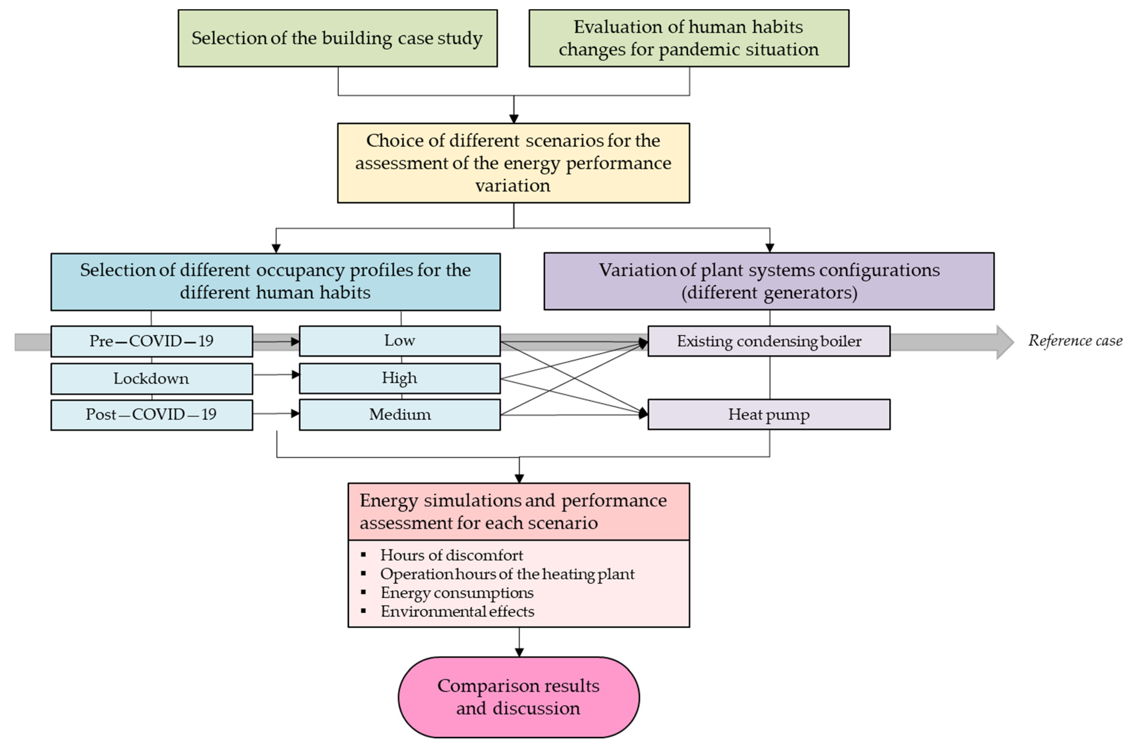
To evaluate the influence of these human habits on building energy consumption, comfort, and environmental aspects, the research followed certain steps (Figure 2), starting from the consideration of the described lifestyles and the selection of a case study deemed representative of a typical and widespread building typology in Italy.
First, three different scenarios of “human habits” were defined, changing the occupancy profiles and the use of appliances and lighting related to them, based on the user behaviours. In this way, the so-called “low” profile was adopted for the pre-COVID-19 lifestyle, the “medium” profile stood for the post-COVID-19 one, and finally the “high” profile for the COVID-19 pandemic period. The terms low, medium, and high were selected to give the idea of occupancy rate in the house, immediately.
At this point, thermal energy simulations were carried out for the analyses of all of the defined scenarios applied to the selected residential case study, which was validated previously in [39]. It was characterized thanks to the available data related to all of the characteristics of the envelope components and plant systems, as well as information about the daily routine of the inhabitant, taking into account the habits of the single occupant, corresponding to the low profile. For this reason, this profile was assumed as the reference case. Thus, the thermophysical characteristics of the case study were implemented in the 3D simulation model and the residential unit was analysed through certified software, implementing the hourly calculation method, according to [32].
The energy simulations were performed by adopting conventional domestic hot water needs and by “setting free” the heating period, to better compare the real energy and environmental effects of the human habits, according to the hourly calculation procedure.
We compared different plant system solutions for each of the three profiles, changing the generator system, to evaluate which better fit the needs of the house occupant, and to highlight whether different human habits could affect the choice of a heat generator system (in case, for instance, of its substitution or renewal).
A comparison between the different analysed scenarios was useful to obtain the variations in terms of discomfort hours, operation hours of the heating plant system, energy consumption, and CO2 emissions, allowing us to understand the influence of the inhabitants’ lifestyles and behavioural changes, before, during, and after COVID-19.
2.1. Hourly Calculation Method
This study is based on a comparison of different human habits simulated with the new energy calculation method, according to UNI EN ISO 52016. Compared to the current energy calculation procedure provided by the UNI TS 11300 series [40,41,42,43], the procedure is capable of assessing the hourly energy needs of a building based on the resistance and capacitor (RC) network thermal model for each building component, i.e., taking into account the thermal inertia of the building envelope.
Currently, the main difference between these two methods consists of the thermal loss evaluation through the building envelope, mainly due to the different time spans for the energy calculation: the UNI TS series provides a monthly energy balance, whilst in UNI EN ISO 52016 it is hourly.
The new procedure provides a less simplified calculation method. In fact, the building envelope must be modelled, as shown in Figure 3, by using 5 nodes with 4 thermal resistances (grey boxes) and by adopting a different number of capacitors (indicated with k in the figure), depending on the position of the mass. This modelling allows accounting of the influence of climate conditions, operation schedules, and thermal inertia of building structures on the energy need assessment. The same is only marginally considered by the UNI TS 11300 series.
According to this description, the energy assessment with the hourly calculation procedure should be more accurate; further studies should be carried out by varying the climatic zones and thermal properties of the building envelope [44]. According to previous papers that analysed the application of the hourly calculation procedure to different types of buildings [33,34,35,36,37,38,44], the energy outcomes significantly varied with the thermal properties of the building envelopes, use of buildings, and outdoor thermal conditions, making a comparison between these works difficult [44].
3. The Case Study
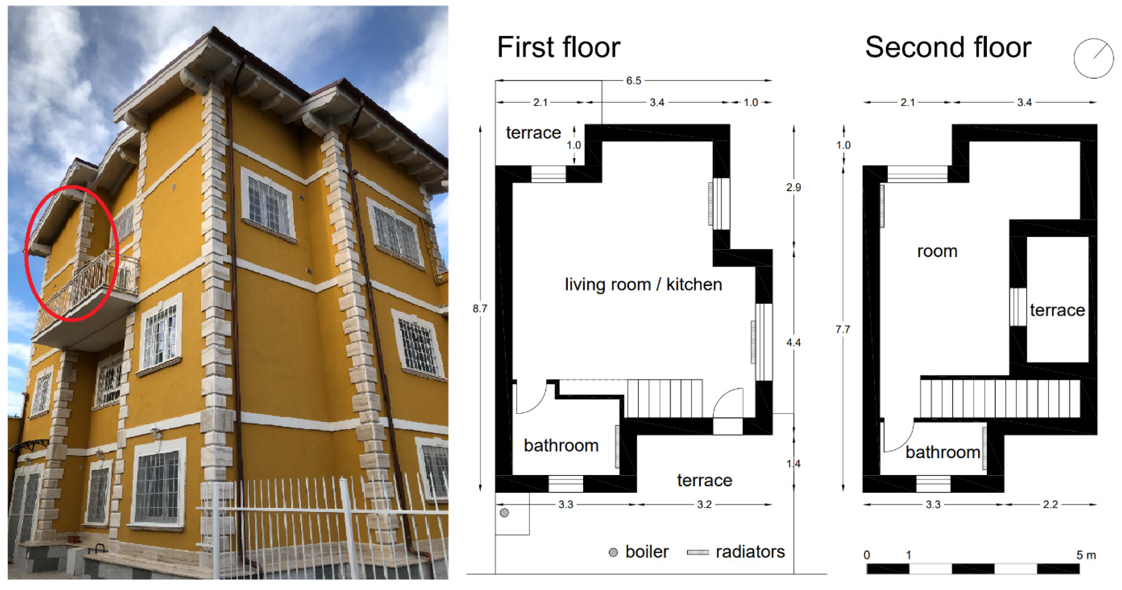
A unit apartment located in a three-storey building in Rome was chosen for the analysis, as representative of a widespread apartment typology. According to [45], the most diffused and best-selling flats have useful areas between 50 and 85 m2, especially in the biggest cities of Italy. Moreover, according to the Italian census (ISTAT), more than five million existing Italian buildings are multi-storey buildings, consisting of various apartments on each floor [46]. The case study has a net surface of 60 m2 and it is located on the second floor of the building, with an independent entrance through external stairs. The apartment has an open space for the kitchen, dining, and living rooms, and a bathroom on the lower floor. Internal stairs lead to the bedroom and the second bathroom on the upper floor (Figure 4).
The north, east, and west facades are external exposed, while the south side adjoins a similar apartment on the same floor.
For the building envelope, the entire building was refurbished in 2019 with a demolition and reconstruction intervention; it is in good agreement with the current standard minimum requirements [47]. It contains a reinforced concrete framed structure with highly insulated walls made of porous brick blocks and expanded polystyrene (EPS) insulation. This kind of insulation is also present in the other building envelope components, such as the roof and the floor ceiling, as illustrated in detail in Table 1.
Openings are characterized by double-glazing and thermal break windows with air gaps and an average transmittance Uw value equal to 1.8 W/m2K.
An independent heating system, consisting of a condensed gas-fired boiler, provides heating and domestic hot water (DHW) production; its rated power is 24 kW with an energy efficiency of 97.7%. A system of radiators with an operating temperature of 70 °C at the inlet section of radiators and 50 °C at the outlet section of radiators, managed by zone thermostats, completes the thermal system. The average delivery temperature of the domestic hot water is 40 °C. No cooling system, or any energy production system by renewable energy sources, was installed in the apartment.
The set point temperatures are fixed to 20 °C in the winter and 26 °C in the summer.
As aforementioned, the energy simulations were carried out in climatic zone D (heating period from 1 November to 15 April), taking, as reference, the city of Rome, characterized by 1642 degree days. The validation of the model was performed by taking into account the real climatic conditions related to the monitored period [39], whilst the current analysis was carried out adopting the climatic data provided by [48] (Figure 5), in order to consider the whole year.
The simulation model was validated previously by adopting two different procedures, as illustrated in [39], by acquiring both billing and indoor environmental conditions, using an experimental campaign, monitoring, and logging indoor environmental conditions (indoor air temperature and relative humidity).
3.1. The Analysed Scenarios
As aforementioned, due to the COVID-19 pandemic, human habits have changed in a relevant way. Occupation is one of the most influencing parameters used in evaluating the energy performance of a house; it is important to understand how great the variations of results are influenced by an occupant’s behaviour. It is essential to hypothesize “realistic” user behaviour and, consequently, a consistent use of plant systems.
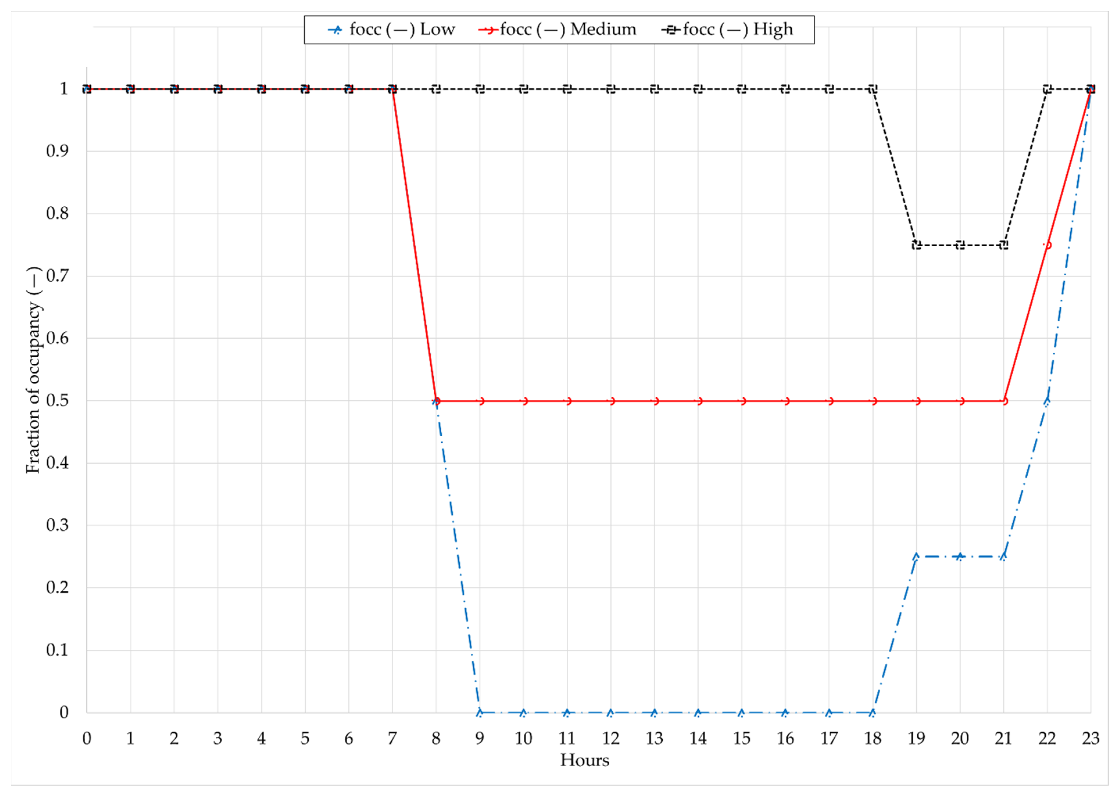
For this reason, the three profiles for the analysed building (Table 2) were hypothesized to cover the three hypotheses of possible user habits and lifestyles (pre-COVID-19, lockdown, and post-COVID-19), described in paragraph 2. A single occupant in the apartment was considered (as in the actual state) and all of the profiles are the results of the average fraction values of occupancy, evaluated in a typical day of the week.
In detail, the so-called “low” profile is characterized by a low occupancy rate of the apartment, more concentrated during evening and night hours, beginning from 19:00 until 7:00 in the morning. It is typical of a young worker, who does not stay in the house during work hours, and is often implied in social and sports activities. Moreover, this profile is calibrated and coherent with the actual use profile of the house monitored in [39], before the COVID-19 pandemic. For this reason, it was assumed as the reference profile for the comparison results.
The second profile was set as medium. It presents a constant probability of occupancy at 50% in the typical day of an apartment inhabitant, and it was chosen according to the legislative standard profile. Moreover, an interview with the occupant confirmed new habits after the COVID-19 pandemic crisis, where the frequency of social and outside activities had decreased to two–three times per week.
The third (and last) profile was set as high, due to the rather constant occupancy of the apartment, except for a little variation during the evening hours (80% of occupancy from 19:00 to 21:00). This is the profile that best fits the last “life months” of the pandemic, which radically changed human habits, with individuals obliging to the lockdown, and due to the reduction of social lives (i.e., for people to avoid being infected). Outside activities were reduced to only needful chores (groceries shopping, medical needs). Moreover, implementation of smart working at home led to long stays in houses, during the central daily hours of a typical day.
The three profiles are illustrated in Figure 6, where value 0 stands for the unoccupied building and value 1 for the fully occupied building.
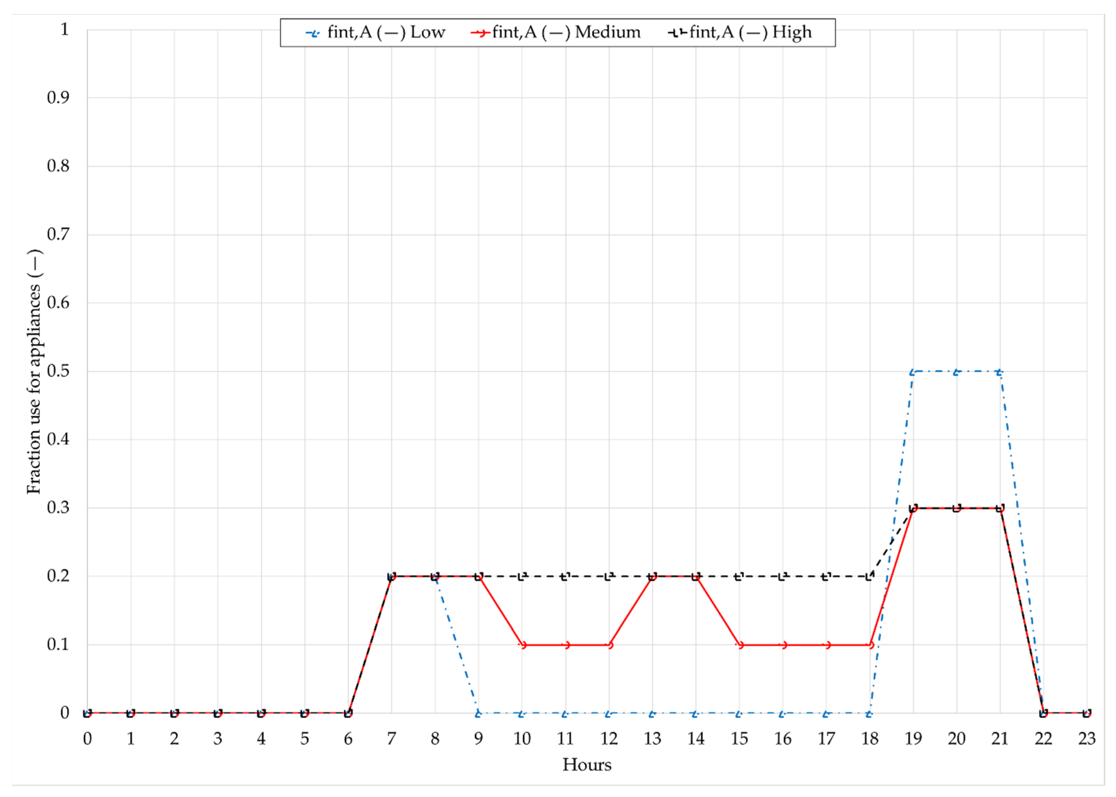
Consistent with occupation, the profiles, regarding use of appliances and lighting systems, varied (Figure 7 and Figure 8). In the low case profile for appliances, it was assumed that they were used during the early hours of the day and during the evening, coherently with the inhabitant’s habits. The general thinking was that, in the low profile, the occupant uses the appliances in the few hours in which he/she stays at home. For this reason, the maximum value of fraction was set to 0.5. In the other profiles, their uses were widespread during the day, with no such peaks, and more regular operation profiles, as evident in Figure 7. This trend correlates with what is affirmed by researchers in [24]; according to the authors, the most important change was that consumption occurred throughout the day instead of being concentrated in the evening, as observed before the lockdown. This is perfectly aligned with the chosen and surveyed scenarios analysed in this work.
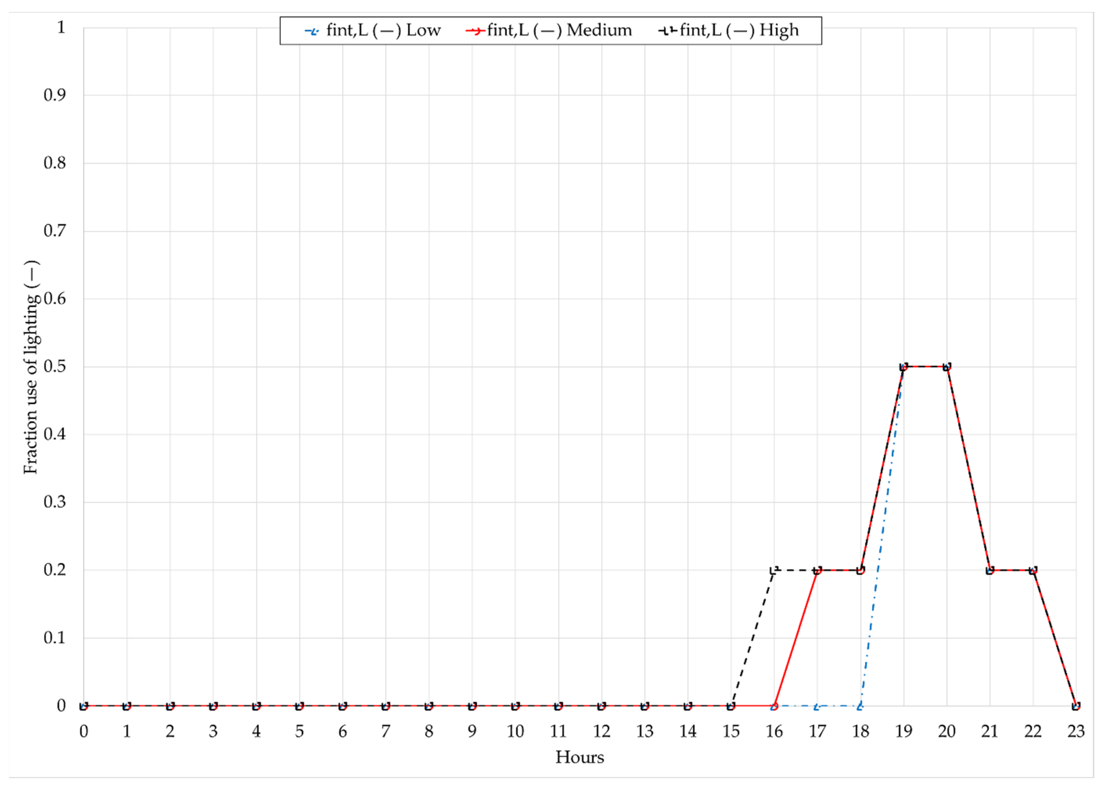
The lighting profiles follow the same consideration of the appliances, but it was calculated as an average period of artificial lighting, beginning from 19:00 for the low profile, and from 17:00 and 16:00 for the medium and high profiles, respectively. Figure 8 shows the trend and the fraction values hour-by-hour.
In relation to the three defined occupancy profiles, specific heat gains were assumed for the people (P), appliances (A), and lighting (L). In absence of measured reliable data for the appliances and for the lighting contribution, the current energy calculation method (that follows UNI TS 11300) proposes an estimation for the sensible and latent contributions; this was assumed in this study. On the other hand, for the sensible heat gain due to the occupant, the same value defined in previous work [39] was adopted. In particular, daily metabolism (Mdaily) was estimated according to the Harris and Benedict relation [49] based on the weight (W expressed in kg), height (H expressed in cm), and years (Y) of the occupant.
Mdaily = 64.730 + 13.7516∙W + 5.0033∙H − 6.7550∙Y (kcal)
As shown in [39], in agreement with the calculated metabolism value, an hourly internal sensible gain due to the occupant, equal to 1.95 W/m2, was considered. The ones due to appliances and lighting were set as 32 and 6 W/m2, respectively [40]. Moreover, the internal heat latent gains were considered, varying hourly, according to the cited profiles of occupancy and appliances, and multiplying them for 2.8 and 12.6 (g/h)/m2 [40].
Table 3 shows the daily values of sensible (indicated with ϕ) and latent (indicated with G) gains for each aspect analysed. As shown, the medium profile has an increase of the internal heat gains of about 42% on average, with respect to the low profile (considered as the reference profile), whilst the high profile is about 84% more than the reference case.
Finally, to evaluate the energy performance of a building, considering the different energy uses derived by the defined profiles, another plant system was hypothesized to define which one best fit the occupant needs.
For this reason, each defined scenario was simulated, substituting the existing condensing boiler with a heat pump. Its sizing was chosen, satisfying the DHW requirements and the heating energy loads according to [39,41]. The heat pump system supplies both the heating and DHW production and has a rated heating capacity of 7.74 kW and a coefficient of performance (COP) of 4.75.
The same typology of emission systems (radiators) was considered for both configurations equal to the reference existing case.
4. Results and Discussion
Energy simulations were performed by setting the three profiles defined in the previous section with the aim of analysing their impacts on:
- Hours of discomfort, evaluated as the number of hours in which the indoor operative temperature was lower (heating), or higher (cooling), than the set point values;
- Energy consumption, analysed as the energy needs of a building for heating, and as a primary energy need (renewable, not renewable, and total), evaluating two heating system configurations described above (condensing boiler and heat pump);
- Operation hours of the heating plant, assessed as the number of hours where the heating system was switched on for reaching the set point temperature within the environment;
- Environmental effects, in term of CO2 emissions varying the heating system configuration.
4.1. Hours of Discomfort
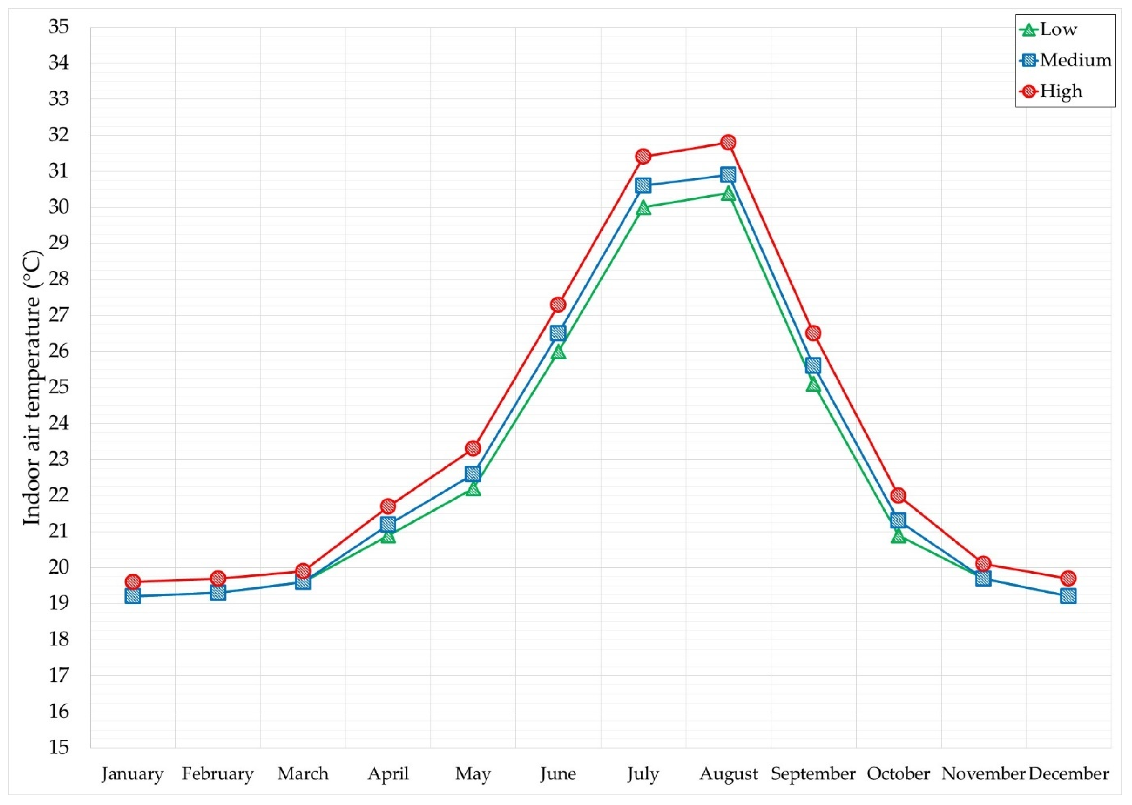
The internal thermal load (returned by energy simulations) of the medium and high profiles are, respectively, (on average) +58% and +149% higher than the internal load of the low profile (reference case), and, according to the UNI EN ISO 52016 calculation method, this affects the indoor air temperature. Figure 9 shows the mean indoor air temperature reached in each month of the year by adopting the low (green line), medium (blue line), and high (red line) occupancy profiles, confirming that the greater the indoor thermal loads (linked to occupancy profiles), the higher the indoor air temperature. In fact, as expected, the mean indoor air temperature tends to increase with the level of occupancy profile (the more time spent in the house, the more internal heat load); in particular, compared to the low profile (reference profile), the increase is up to 2.0% and to 5.6% for medium and high profiles, respectively. Nevertheless, the indoor air temperatures obtained with medium and low profiles tend to correspond during the coldest months (from November to February) although the indoor thermal load of the medium profile is higher (about +55%, considering only the heating period). On the other hand, the high profile gives an air temperature trend shift of at least 0.5 °C in the coldest months.
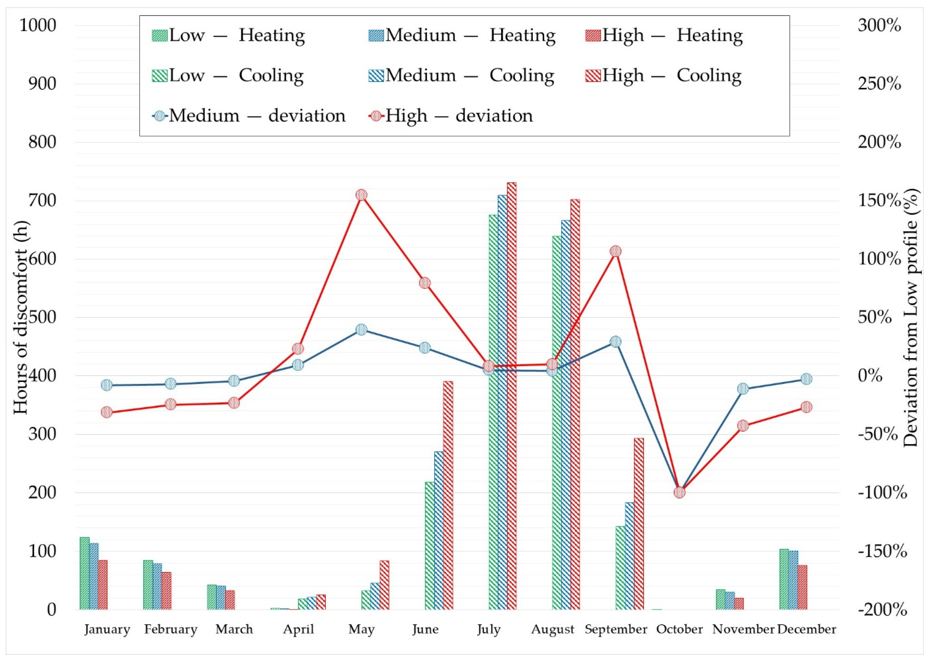
Furthermore, the mean indoor air temperature involves different discomfort levels within the environment. As shown in Figure 10, the reference profile (i.e., the low profile, indicated with green bars) leads to a higher number of hours of discomfort during the heating period (about 390 h), whilst it leads to a lowest number of hours of discomfort during the cooling seasons (less than 1900 h). The medium profile allows reducing the hours of discomfort during the heating period, of about 11% on average, with peaks over the intermediate months (April and October). A higher significant reduction, up to 45%, on average, can reached during the heating period, by adopting a high occupancy profile. However, both profiles (medium and high) led to a significant increase of the hours of discomfort during the cooling period, of about 24% and 80%, respectively. In the spring and autumn months, a higher deviation was found, especially for the high profile, which could increase up to +154% (May). This result indicates that, in the intervening months, even small temperature deviations can lead to significant levels of discomfort within the environment.
Another important consequence is related to the application of the hourly calculation method. In fact, as aforementioned, the building is equipped by an existing HVAC system, which was designed with current energy regulations [40,41,42,43,50], and refers to the monthly calculation procedures for which the building solely has heating needs. According to Figure 9 and Figure 10 (which refer to hourly calculation procedures), cooling is also necessary due to both the higher mean values of temperatures reached indoors (more than 30 °C) and the high number of hours of discomfort found from June to September. This result confirms the capability of the new hourly calculation method of providing more accurate energy analysis of HVAC systems. In fact, it takes into account the time lag between the switch-on time of an HVAC system and the time of the required set point temperature; therefore, it helps to analyse whether the system is over- or undersized.
4.2. Building Energy Need
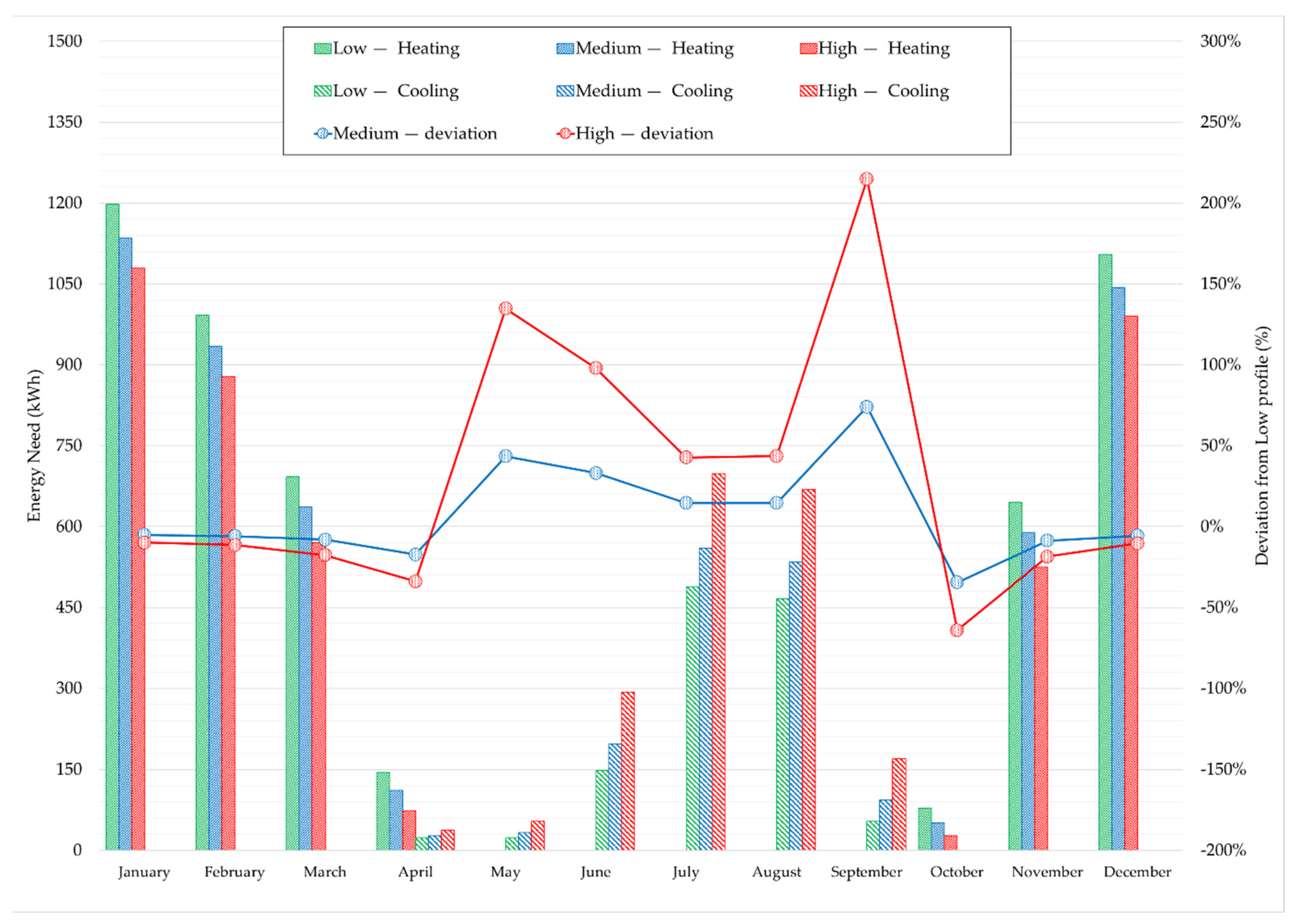
The indoor air temperature reached within the environment and the number of hours of discomfort are directly (and strictly) linked to the energy needs for heating and cooling. In fact, the lower the discomfort (corresponding to higher indoor air temperature), the less the energy need for heating (Figure 11); the higher the discomfort (corresponding to higher indoor air temperature), the greater the energy need for cooling (Figure 11). Therefore, according to Figure 11, compared to the reference profile (i.e., low profile), the high occupancy one allows reducing the energy need for heating of about 15% on average, but it leads to a significant increase of an energy need for cooling, up to 60% on average. The medium occupancy profile, instead, allows reducing the energy need for heating of about 7%, involving an increase of an energy need for cooling of 20%. As for the hours of discomfort, and for the energy need, the higher deviations, with respect to the baseline profile, were found in the intervening months (especially in June and September).
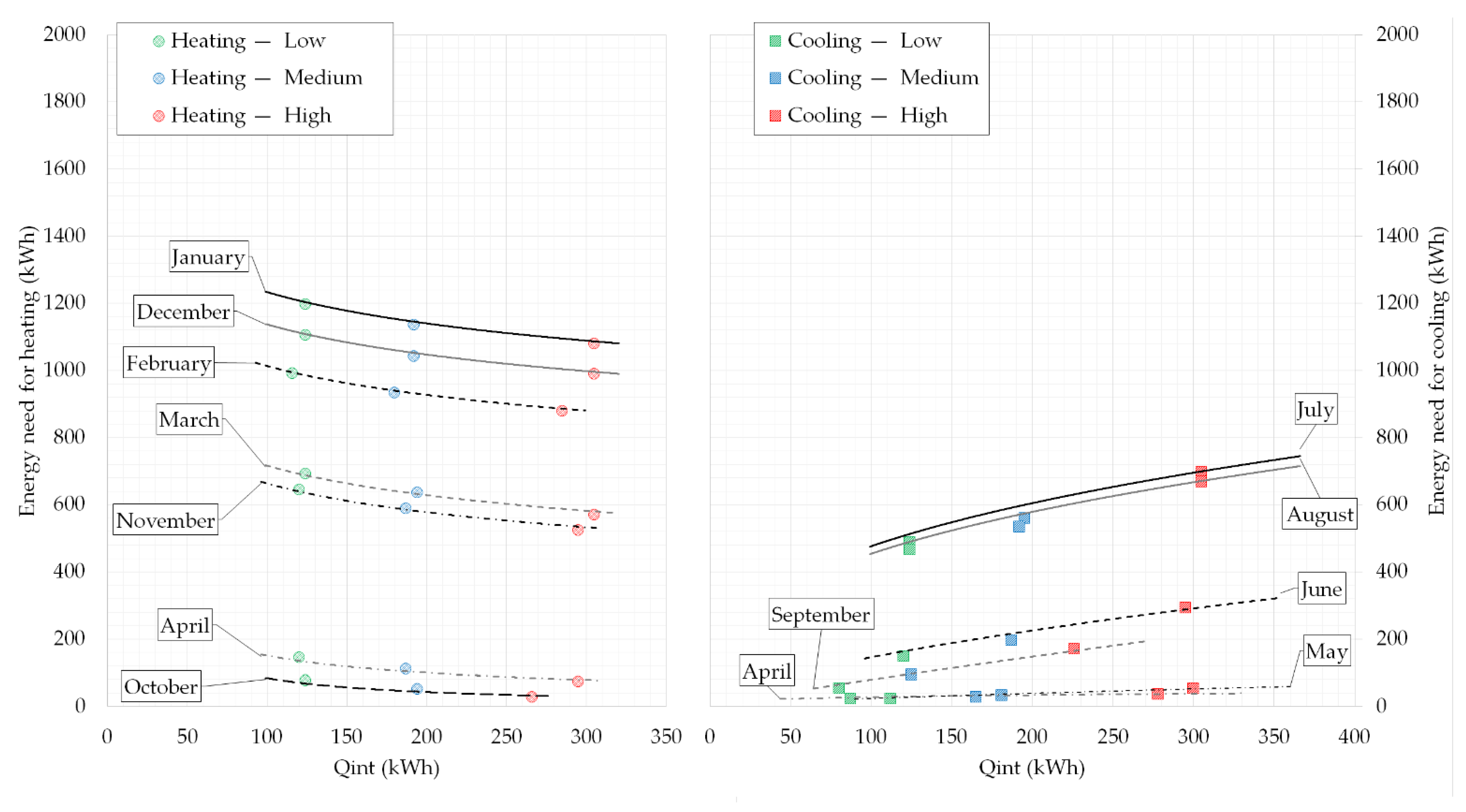
A more accurate analysis of the energy needs as functions on the occupancy profiles is shown in Figure 12. In particular, the energy need for heating and for cooling were analysed with respect to indoor thermal loads (Qint), where the low profile is indicated with the green series, medium with the blue ones, and high with the red series. Dots, referring to the same months, are joined through the same curve; they represent monthly values of energy needs for the heating and cooling periods for each case. As highlighted, the energy need for heating tends to decrease with the increase of Qint, the opposite can be observed for the cooling period.
This trend can also be explained by relating the hours of discomfort with the energy needs of the three occupancy profiles. As shown in Figure 13, the linear regression line (red line) for heating months is more tilted than the cooling period (blue line), confirming that the hours of discomfort during the heating period have greater influence on the energy needs of buildings. Even in this figure, each dot represents the different months of the cooling and heating periods, and they are drawn with different symbols (corresponding to the three investigated scenarios) and with different backgrounds (corresponding to different months).
4.3. Operation of Heating System
The indoor air temperature reached within the environment, the hours of discomfort, and the energy needs of the building, also have considerable influence on the operation of the heating system (the case study only has the heating and domestic hot water production system). For further analysis, the operation hours of the heating system were studied compared to the occupancy profiles and to the heating system load factor (HLF). The analysis (Figure 14) highlighted that a high occupancy profile leads to a lower number of hours at HLF > 75% (less than 25%), and at HLF between 50 and 75% (about 17%), with a consequent increase of operating hours, mainly at HLF in the 25–50% range (up to 34%). A similar trend can be observed for the medium profile, but with slightly less significant deviation compared to the low profile. This result has important consequences, because it highlights that, by varying the occupancy profile, the performance of the heating system can significantly vary, determining a possible worse performance of the heating system. Moreover, based on the high and medium occupancy profiles, it can be concluded that the power of the heating system could be oversized, resulting in the need of using a heating system with lower thermal power than the one required for the low profile. The same results are detailed in Table 4, where the effective number of operating hours of the heating plant are shown.
Finally, the energy performance with the different heating systems was also analysed; results are summarized in Table 5, in terms of primary energy need (kWh) and energy carrier consumption (natural gas and electric energy). As expected, the configuration with the heat pump is the one with the higher renewable contribution (ren), which decreases from a low to a high profile, mainly due to the reduction of the energy needs of the building. The lowest energy carrier consumption was always obtained with the high profile; compared to the low profile, natural gas was reduced up to 13% for the condensing boiler.
4.4. Environmental Effects
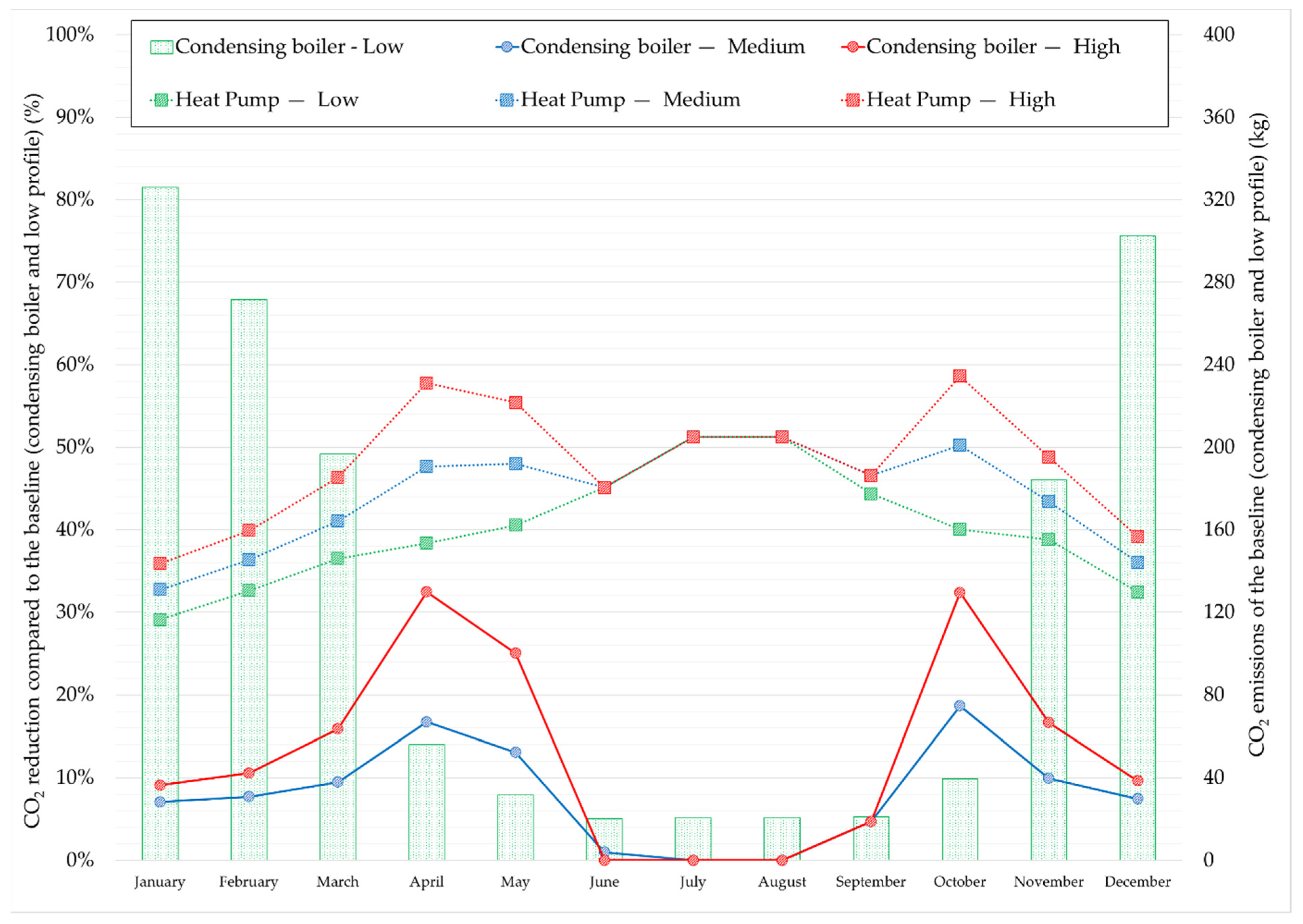
Finally, the environmental effects were investigated. Results are shown in Figure 15, where the reduction of CO2 emissions, compared to the reference case (i.e., condensing boiler and low profile) are highlighted as functions of occupancy profiles (low indicated with the green series, medium with the blue, and high the with red series), and plant system configurations (the condensing boiler is indicated with the circle symbol, the heat pump with square ones). As shown, compared to the reference case, the high profile allows obtaining a CO2 reduction of about 52% on average with the heat pump. Similar reductions were found by adopting the medium profile (49% on average). On the other hand, if the actual plant configuration is considered (but with a different occupancy scenario), a similar reduction can be noticed; specifically, the high occupancy profile allows reducing the CO2 emission of about 13–15%, while the medium one of about 7–8% on average.
This result highlights the great influence of the occupancy profile on environmental affects, entailing differences, especially in the intervening months.
5. Conclusions
This paper compared the effects of lifestyle variations of an inhabitant in a real dwelling, before and after the pandemic, on: (i) the total number of discomfort hours; (ii) the energy needs of the case study; (iii) the operation of the heating system; and (iv) the environmental effects.
In regard to the hour of discomfort, the results mainly show that:
- The increase in the number of hours spent indoors (from low to high occupancy) causes an increase in indoor temperature (up to 2 °C in August). However, a significant variation in internal loads (+58% and +149%) causes a slight variation (about 1–2%) of the indoor air temperature during the heating period and a variation of up to 4–5% during the cooling period. This implies an increase in discomfort hours during the summer, and a decrease during the winter. In June and September, there is a higher absolute difference of discomfort hours.
- During the heating season, the maximum number of discomfort hours (124) is registered in January for the low occupancy profile, whilst during the cooling season, the maximum number of discomfort hours (731) is registered in July for the high occupancy profile.
The energy needs for heating and cooling, simulated with the new hourly calculation method, highlight that:
- The energy need for cooling in the case study is much lower than the heating load, and it is concentrated in July (266 operation hours) and August (271 operation hours), on a total of 737 h working hours (for the cooling season). This implies a daily average turning-on of 8 h.
- The building energy need varies according to the occupancy, appliances, and lighting profiles, but higher deviations (almost 300%) are found for the summer months. This implies that these schedules mainly affect the cooling load. This result was confirmed by analysing the energy need as a function of the internal load. Moreover, it is consistent with some outcomes in the literature studies, such as [30], where the researchers sustain that, if the lockdown occurred in the summer, the long stay of people at home and the long use of electrical appliances would increase the overheating issues and the internal heat gains. Consequently, it could force the building owners to install cooling systems to achieve thermal comfort, causing a significant change in the energy breakdown of buildings.
By combining the results of these two first topics, the operation hours of the HVAC system were analysed, finding that the different scenarios could affect the operation hours of the heating plant:
- As per the HVAC system, when the occupancy is high, it will work for many hours when the load is <50%. On the contrary, when the occupancy is low, the HVAC system will work for many hours with a high load (>50%).
- The plant system can work at the lower load factor value, entailing an oversizing of the heating system, which can operate with lower energy efficiency.
Given the considerations above on the operation hours and on the load, it is worth comparing the different heating and DHW systems, in terms of primary energy needs and environmental effects:
- The condensing boiler with a high occupancy profile has a lower total primary energy need, whilst the higher value is reached by the heat pump working with low occupancy. This implies an overall consideration: in case, for example, there is a need to renovate the HVAC system, its choice should be conducted according to the foreseeable occupancy profile of the building.
- The occupancy profile significantly affects the primary energy need and the consumptions of the energy carriers. The high profile, i.e., homemaker or a person who spends much time at home (linked also to the COVID-19 pandemic period), entails a lower primary energy need and lower energy consumption (of about 12%), allowing to reduce the CO2 emissions of about 12%, considering condensing the boiler and heat pump. This could be in disagreement with some studies, which registered an overall increase in the residential sector during the lockdown [26,30]. This work provides an in-depth analysis of building heating system operations, which is useful to understand how different occupancy scenarios could foster the reduction of general consumption. In order to estimate, in detail, the differences in energy consumption (thus considering the economic effects of appliance schedule), an overall point of view is necessary, in relation to the different building sectors (non-residential and residential), and obtaining the total consumptions before and after the pandemic, as conducted by other authors in [27,51].
- The high occupancy profile allows CO2 reduction (with respect to the reference case) of about 52%, on average, with the heat pump.
From all of these considerations, it is evident how the pandemic has influenced the habits of owners and inhabitants in buildings and, consequently, the energy consumptions of the buildings themselves. Overall, it could be highlighted that the changes have affected quality of life, not only in terms of thermal comfort, but also in regard to notable environmental impacts. Moreover, energy consumption, increased in the summer and reduced in the winter, influences the billing and related costs; this determines that the involved stakeholders (building owners, landlords, inhabitants, etc.) must adopt more conscious behaviour in their houses, for energy savings.
Finally, the analysis carried out in this research can be useful to policymakers in accomplishing the European objectives (such as a decarbonized building stock by 2050). They have to calibrate their decisions in terms of long-term strategies, taking into account the changes in human life, for example, promoting, as a starting point, the recognition of building stock consumption in light of after-pandemic changes, and promoting informative campaigns for user awareness, and new thresholds for energy consumption. Moreover, the issue of increasing cooling needs—which has improved in the last few years due to climate change—as well as issues surrounding heat waves and global warming, are risks that will continue to grow, as a result of the long stays at home. Thus, it could be useful to promote outside activities in the summer and incentives for working in suitable spaces, designed specifically for the optimization of HVAC systems, lighting, and electrical equipment, which are often not effective for working in houses.
Final Remarks
The research questions are: (i) how many discomfort hours could there be in the different occupancy scenarios? (ii) How much does an occupancy profile change a building’s total energy consumption? (iii) How much do human habits (and the new schedules due to the pandemic) influence the CO2 emissions of a building?
To answer to the first research question, the yearly discomfort hours range from 279 (in the high occupancy scenario) to 395 (in the low occupancy scenario). During the heating and the cooling periods, the ranges are 1–85 and 1–124.
In answer to the second question, the occupancy profile can affect the operation hours and the building final energy consumption, up to 28% on average, with peaks up to 215% in the intervening months.
The third answer assesses that a new schedule for a high occupancy profile (due, for instance, to containment for a pandemic) can reduce the building CO2 emission of about 13%.
As a final remark, it is worth noting that the building was designed and built complying with the rules of standard UNI TS 11300, which calculates the building energy needs by a monthly average base, and according to which the building does not require energy for cooling. This work, indeed, is carried out following UNI EN ISO 52016, which elaborates an hourly calculation and performs a discomfort analysis, highlighting a cooling energy need (1200 kWh), mainly concentrated in July and August.
Hence, the new energy calculation method (UNI EN ISO 52016) provides results that better fit the real need (also considering the inhabitant need).
Finally, the aim of the work was to assess the implication of different HVAC systems. Indeed, the promoted renovation of HVAC systems (in favour, for instance, of a heat pump) should properly consider the human habits of the occupant. This is also in the case of “human habit permanent change”, which is likely to occur, considering that some restrictions and limitations are still in force.
Hence, when a building heating system must be replaced, evaluation on it use, and on the inhabitant’s schedule, should be carried out. This is also to avoid some common setbacks, such as plant (or system) oversizing, or system load factors far from maximum efficiency. These drawbacks, indeed, might affect the economic and environmental benefits of the chosen system.
6. Limitations and Future Works
The study was possible because of the detailed knowledge of the building itself (geometry, architectural, and constructive features, plant system characteristics, etc.), and inhabitant behaviours (occupancy profiles, lighting, and appliance schedules).
These considerations are related to the investigated case study; in order to overcome this limitation and to extend the outcomes, further studies should be conducted (for instance, evaluating the heating and cooling energy needs with electrical consumptions derived by domestic appliances).
Author Contributions
Conceptualization and methodology, D.P., S.D.T. and I.N.; software and validation, D.P.; data curation, D.P.; writing—original draft preparation, D.P., S.D.T. and I.N.; writing—review and editing, D.P., S.D.T. and I.N. All authors have read and agreed to the published version of the manuscript.
Funding
This research received no external funding.
Institutional Review Board Statement
Not applicable.
Informed Consent Statement
Not applicable.
Data Availability Statement
The data presented in this study is from a new design analysis carried out in line with the objective of the study. All the data is available under request to the corresponding Authors.
Conflicts of Interest
The authors declare no conflict of interest.
Abbreviations
| Symbol | |
| CO2 | carbon dioxide |
| COP | coefficient of performance |
| cp | specific heat |
| DHW | domestic hot water |
| f | fraction |
| ϕ | sensible heat gain |
| G | latent heat gain |
| HLF | heating load factor |
| HVAC | heating, ventilation and air-conditioning system |
| λ | thermal conductivity |
| M | metabolism |
| ρ | density |
| R | thermal Resistance |
| t | thickness |
| U | thermal transmittance |
| Subscripts | |
| A | appliances |
| int | internal heat gain |
| L | lighting |
| occ | occupancy |
| P | people |
References
- International Energy Agency (IEA). Tracking Building 2020; IEA: Paris, France, 2020; Available online: https://www.iea.org/reports/tracking-buildings-2020 (accessed on 27 August 2021).
- Motuziene, V.; Vilutiene, T. Modelling the effect of the domestic occupancy profiles on predicted energy demand of the energy efficient house. Procedia Eng. 2013, 57, 798–807. [Google Scholar] [CrossRef] [Green Version]
- Flett, G.; Kelly, N. Modelling of individual domestic occupancy and energy demand behaviours using existing datasets and probabilistic modelling methods. Energy Build. 2021, 252, 111373. [Google Scholar] [CrossRef]
- Akbari, S.; Haghighat, F. Occupancy and occupant activity drivers of energy consumption in residential buildings. Energy Build. 2021, 250, 111303. [Google Scholar] [CrossRef]
- Ali, Q.; Thaheem, M.J.; Ullah, F.; Sepasgozar, S.M.E. The performance gap in energy-efficient office buildings: How the occupants can help? Energies 2020, 13, 1480. [Google Scholar] [CrossRef] [Green Version]
- Di Turi, S.; Falcone, I.; Nardi, I.; Ronchetti, L.; Calabrese, N. Evaluation of the energy performance of Zero Energy residential Buildings: Complexity of dynamic simulations and results variability. E3S Web Conf. 2021, 312, 06002. [Google Scholar]
- Louis, J.N.; Caló, A.; Leiviskä, K.; Pongrácz, E. Modelling home electricity management for sustainability: The impact of response levels, technological deployment & occupancy. Energy Build. 2016, 119, 218–232. [Google Scholar]
- D’Oca, S.; Hong, T. Occupancy schedules learning process through a data mining framework. Energy Build. 2015, 88, 395–408. [Google Scholar] [CrossRef] [Green Version]
- Santin, O.G. Behavioural patterns and user profiles related to energy consumption for heating. Energy Build. 2011, 43, 2662–2672. [Google Scholar] [CrossRef]
- Zambrano, J.M.; Oberegger, U.F.; Salvalai, G. Towards integrating occupant behaviour modelling in simulation-aided building design: Reasons, challenges and solutions. Energy Build. 2021, 253, 111498. [Google Scholar] [CrossRef]
- Causone, F.; Carlucci, S.; Ferrando, M.; Marchenko, A.; Erba, S. A data-driven procedure to model occupancy and occupant-related electric load profiles in residential buildings for energy simulation. Energy Build. 2019, 202, 109342. [Google Scholar] [CrossRef]
- Alonso, M.; Rubio, A.; Escrig, T.; Soto, T.; Serrano-Lanzarote, B.; Matarredona-Desantes, N. Identification of measures to strengthen resilience in homes on the basis of lockdown experience during COVID-19. Sustainability 2021, 13, 6168. [Google Scholar] [CrossRef]
- Awada, M.; Becerik-Gerber, B.; Hoque, S.; Zheng, O.; Giulia, P.; Jin, W.; Teresa, W. Ten questions concerning occupant health in buildings during normal operations and extreme events including the COVID-19 pandemic. Build. Environ. 2021, 188, 107480. [Google Scholar] [CrossRef]
- Strielkowski, W.; Firsova, I.; Lukashenko, I.; Raudeliūniene, J.; Tvaronavičiene, M. Effective management of energy consumption during the COVID-19 pandemic: The role of ICT solutions. Energies 2021, 14, 893. [Google Scholar] [CrossRef]
- Abdeen, A.; Kharvari, F.; O’Brien, W.; Gunay, B. The impact of the COVID-19 on households’ hourly electricity consumption in Canada. Energy Build. 2021, 250, 111280. [Google Scholar] [CrossRef]
- Cortiços, N.D.; Duarte, C.C. COVID-19: The impact in US high-rise office buildings energy efficiency. Energy Build. 2021, 249, 111180. [Google Scholar] [CrossRef] [PubMed]
- Qarnain, S.S.; Sattanathan, M.; Sankaranarayanan, B.; Ali, S.M. Analyzing energy consumption factors during coronavirus (COVID-19) pandemic outbreak: A case study of residential society. Energy Sources Part A Recover Util. Environ. Eff. 2020, 1–20. [Google Scholar] [CrossRef]
- Qarnain, S.S.; Muthuvel, S.; Bathrinath, S. Review on government action plans to reduce energy consumption in buildings amid COVID-19 pandemic outbreak. Mater. Today Proc. 2021, 45, 1264–1268. [Google Scholar] [CrossRef]
- Cvetković, D.; Nešović, A.; Terzić, I. Impact of people’s behavior on the energy sustainability of the residential sector in emergency situations caused by COVID-19. Energy Build. 2021, 230, 110532. [Google Scholar] [CrossRef] [PubMed]
- Kolakowski, H.; Shepley, M.M.; Valenzuela-Mendoza, E.; Ziebarth, N.R. How the COVID-19 Pandemic Will Change Workplaces, Healthcare Markets and Healthy Living: An Overview and Assessment. Sustainability 2021, 13, 10096. [Google Scholar] [CrossRef]
- Petcu, M.A.; Sobolevschi-David, M.I.; Anica-Popa, A.; Curea, S.C.; Motofei, C.; Popescu, A.M. Multidimensional assessment of job satisfaction in telework conditions. Case study: Romania in the covid-19 pandemic. Sustainability 2021, 13, 8965. [Google Scholar] [CrossRef]
- Aruga, K.; Islam, M.M.; Jannat, A. Does staying at home during the covid-19 help reduce CO2 emissions? Sustainability 2021, 13, 8534. [Google Scholar] [CrossRef]
- Geraldi, M.S.; Bavaresco, M.V.; Triana, M.A.; Melo, A.P.; Lamberts, R. Addressing the impact of COVID-19 lockdown on energy use in municipal buildings: A case study in Florianópolis, Brazil. Sustain. Cities Soc. 2021, 69, 102823. [Google Scholar] [CrossRef] [PubMed]
- Krarti, M.; Aldubyan, M. Review analysis of COVID-19 impact on electricity demand for residential buildings. Renew. Sustain. Energy Rev. 2021, 143, 110888. [Google Scholar] [CrossRef]
- Jiang, P.; Van Fan, Y.; Klemeš, J.J. Impacts of COVID-19 on energy demand and consumption: Challenges, lessons and emerging opportunities. Appl. Energy 2021, 285, 116441. [Google Scholar] [CrossRef] [PubMed]
- Monzón-Chavarrías, M.; Guillén-Lambea, S.; García-Pérez, S.; Montealegre-Gracia, A.L.; Sierra-Pérez, J. Heating energy consumption and environmental implications due to the change in daily habits in residential buildings derived from COVID-19 crisis: The case of Barcelona, Spain. Sustainability 2021, 13, 918. [Google Scholar] [CrossRef]
- Kang, H.; An, J.; Kim, H.; Ji, C.; Hong, T.; Lee, S. Changes in energy consumption according to building use type under COVID-19 pandemic in South Korea. Renew. Sustain. Energy Rev. 2021, 148, 111294. [Google Scholar] [CrossRef] [PubMed]
- Ghiani, E.; Galici, M.; Mureddu, M.; Pilo, F. Impact on electricity consumption and market pricing of energy and ancillary services during pandemic of COVID-19 in Italy. Energies 2020, 13, 3357. [Google Scholar] [CrossRef]
- Nardi, I.; Palladino, D. How pandemic affects occupants’ buildings perception: Questionnaires investigation and preliminary results. E3S Web Conf. 2021, 312, 02011. [Google Scholar]
- Rouleau, J.; Gosselin, L. Impacts of the COVID-19 lockdown on energy consumption in a Canadian social housing building. Appl. Energy 2021, 287, 116565. [Google Scholar] [CrossRef]
- Mokhtari, R.; Jahangir, M.H. The effect of occupant distribution on energy consumption and COVID-19 infection in buildings: A case study of university building. Build. Environ. 2021, 190, 107561. [Google Scholar] [CrossRef] [PubMed]
- Italian National Unification Body (UNI); European Standardization (EN); International Organization for Standardization (ISO). UNI EN ISO 52016-1: 2018. Energy performance of buildings-Energy Needs for Heating and Cooling, Internal Temperatures and Sensible and Latent Heat Loads-Part 1: Calculation Procedures; Italian National Unification Body (UNI): Milan, Italy, 2018. [Google Scholar]
- Bruno, R.; Bevilacqua, P.; Arcuri, N. Assessing cooling energy demands with the EN ISO 52016-1 quasi-steady approach in the Mediterranean area. J. Build. Eng. 2019, 24, 100740. [Google Scholar] [CrossRef]
- Ohlsson, A.K.E.; Olofsson, T. Benchmarking the practice of validation and uncertainty analysis of building energy mod-els. Renew. Sustain. Energy Rev. 2021, 142, 110842. [Google Scholar] [CrossRef]
- Summa, S.; Tarabelli, L.; Di Perna, L. Evaluation of ISO 52010-1: 2017 and proposal for an alternative calculation procedure. Solar Energy 2021, 218, 262–281. [Google Scholar] [CrossRef]
- Congedo, P.M.; Baglivo, C.; Centonze, G. Walls comparative evaluation for the thermal performance improvement of low-rise residential buildings in warm Mediterranean climate. J. Build. Eng. 2020, 28, 101059. [Google Scholar] [CrossRef]
- Mazzarella, L.; Scoccia, R.; Colombo, P.; Motta, M. Improvement to EN ISO 52016-1:2017 hourly heat transfer through a wall assessment: The Italian National Annex. Energy Build. 2020, 210, 109758. [Google Scholar] [CrossRef]
- Palladino, D.; Scrucca, F.; Calabrese, N.; Barberio, G.; Ingrao, C. Durum-Wheat Straw Bales for Thermal Insulation of Buildings: Findings from a Comparative Energy Analysis of a Set of Wall-Composition Samples on the Building Scale. Energies 2021, 14, 5508. [Google Scholar] [CrossRef]
- Palladino, D.; Nardi, I. Approaching the validation of building energy models: Billing vs indoor environmental data. E3S Web Conf. 2020, 197, 02001. [Google Scholar] [CrossRef]
- Italian National Unification Body (UNI). UNI TS 11300—Part 1: 2014. Energy Performance of Buildings: Evaluation of Energy Need for Space Heating and Cooling; Italian National Unification Body (UNI): Milan, Italy, 2014. [Google Scholar]
- Italian National Unification Body (UNI). UNI TS 11300—Part 2: 2019. Energy Performance of Buildings: Evaluation of Primary Energy Need and of System Efficiencies for Space Heating, Domestic Hot Water Production, Ventilation and Lighting for Non-Residential Buildings; Italian National Unification Body (UNI): Milan, Italy, 2019. [Google Scholar]
- Italian National Unification Body (UNI). UNI TS 11300—Part 3: 2010. Energy Performance of Buildings: Evaluation of Primary Energy Need and of System Efficiencies for Cooling; Italian National Unification Body (UNI): Milan, Italy, 2010. [Google Scholar]
- Italian National Unification Body (UNI). UNI TS 11300—Part 4: 2016. Energy Performance of Buildings: Renewable Energy and Other Generation Systems for Space Heating and Domestic Hot Water Production; Italian National Unification Body (UNI): Milan, Italy, 2016. [Google Scholar]
- Palladino, D.; Iatauro, D.; Signoretti, P. Application of hourly dynamic method for nZEB buildings in Italian context: Analysis and comparisons in national calculation procedure framework. E3S Web Conf. Volume 2021, 312, 02006. [Google Scholar]
- Divisione Servizi Direzione Centrale Servizi Estimativi and Osservatorio Mercato Immobiliare, “Real estate report 2019. Residential Sector” 23rd may 2019 (reference period: 2018). Italian only. Available online: https://www.agenziaentrate.gov.it/portale/web/guest/schede/fabbricatiterreni/omi/pubblicazioni/rapporti-immobiliari-residenziali (accessed on 10 March 2020).
- Censimento Popolazione Abitazioni, Istat. 2011. Italian only. Available online: http://dati-censimentopopolazione.istat.it/Index.aspx (accessed on 18 March 2020).
- Ministerial Decree 26 June 2015: Application of the Methodologies for Calculating Energy Performance and Definition of the Details and Minimum Requirements of Buildings. 2015. Italian only. Available online: https://www.gazzettaufficiale.it/eli/id/2015/07/15/15A05199/sg (accessed on 15 September 2021).
- Italian National Unification Body (UNI). UNI 10349-1: 2016. Heating and Cooling in Buildings—Climatic Data-Part 1: Monthly Means for Evaluation of Energy Need for Space Heating and Cooling and Methods for Splitting Global Solar Irradiance into the Direct and Diffuse Parts and for Calculate the Solar Irradiance on Tilted Planes; Italian National Unification Body (UNI): Milan, Italy, 2016. [Google Scholar]
- Harris, J.A.; Benedict, F.G. A biometric study of human basal metabolism. Proc. Natl. Acad. Sci. USA 1918, 4, 370–373. [Google Scholar] [CrossRef] [PubMed] [Green Version]
- Italian National Unification Body (UNI). UNI EN 12831-1: 2018. Energy performance of buildings—Method for Calculation of the Design Heat Load-Part 1: Space Heating Load, Module M3-3; Italian National Unification Body (UNI): Milan, Italy, 2018. [Google Scholar]
- García, S.; Parejo, A.; Personal, E.; Guerrero, J.I.; Biscarri, F.; León, C. A retrospective analysis of the impact of the COVID-19 restrictions on energy consumption at a disaggregated level. Appl. Energy 2021, 287, 116547. [Google Scholar] [CrossRef] [PubMed]
Figure 1.
Change of human habits before, during, and after the COVID-19 pandemic.

Figure 2.
Methodology.

Figure 3.
Re-elaboration of the scheme of resistance and capacitor (RC) network thermal model provided by UNI EN 52016 [32].
Figure 3.
Re-elaboration of the scheme of resistance and capacitor (RC) network thermal model provided by UNI EN 52016 [32].

Figure 4.
View and plans of the analysed case study.

Figure 5.
Monthly average values of temperature and global solar irradiance on the horizontal surface.
Figure 5.
Monthly average values of temperature and global solar irradiance on the horizontal surface.

Figure 6.
Occupancy fraction profiles for the different scenarios analysed (low, medium, and high).

Figure 7.
Fraction of appliance uses for the different scenarios analysed (low, medium, and high).

Figure 8.
Fraction of lighting use for the different scenarios analysed (low, medium, and high).

Figure 9.
Indoor air temperature reached within the environment by adopting the three defined profiles.
Figure 9.
Indoor air temperature reached within the environment by adopting the three defined profiles.

Figure 10.
Number of discomfort hours simulated within the environment during the heating period for the three defined profiles.
Figure 10.
Number of discomfort hours simulated within the environment during the heating period for the three defined profiles.

Figure 11.
Energy needs for heating and for cooling in the three scenarios.

Figure 12.
Heating and cooling energy needs as functions of the indoor thermal loads due to the individuals in the three scenarios.
Figure 12.
Heating and cooling energy needs as functions of the indoor thermal loads due to the individuals in the three scenarios.

Figure 13.
Energy needs for heating and for cooling compared to the hours of discomfort for the three scenarios.
Figure 13.
Energy needs for heating and for cooling compared to the hours of discomfort for the three scenarios.

Figure 14.
Operation hour percentage (%) during the heating season for different load factor ranges and profiles: (a) lower than 25%, (b) between 25 and 50%, (c) between 50 and 75%, and (d) greater than 75%.
Figure 14.
Operation hour percentage (%) during the heating season for different load factor ranges and profiles: (a) lower than 25%, (b) between 25 and 50%, (c) between 50 and 75%, and (d) greater than 75%.

Figure 15.
Environmental effects due to the different analysed profiles and heating and domestic hot water production system configurations.
Figure 15.
Environmental effects due to the different analysed profiles and heating and domestic hot water production system configurations.


Table 1.
Thermal and geometric characteristics of the opaque building envelope.
| Typology | Materials | t (m) | λ (W/mK) | cp (kJ/kgK) | ρ (kg/m3) | R (m2K/W) | U (W/m2K) |
|---|---|---|---|---|---|---|---|
| External Walls | External gypsum plaster | 0.020 | 0.180 | 1.000 | 600 | 0.111 | 0.231 |
| Porous brick blocks | 0.250 | 0.325 | 0.840 | 748 | 0.769 | ||
| EPS insulation | 0.120 | 0.037 | 1.450 | 15 | 3.243 | ||
| Internal plaster | 0.100 | 0.300 | 0.840 | 1300 | 0.033 | ||
| Roof | Shingles | 0.020 | 0.575 | 2.200 | 1350 | 0.035 | 0.194 |
| Wooden plank | 0.040 | 0.120 | 2.200 | 450 | 0.333 | ||
| EPS insulation | 0.160 | 0.0370 | 1.450 | 15 | 4.324 | ||
| Wooden plank | 0.040 | 0.120 | 2.200 | 450 | 0.333 | ||
| Ceiling | Floor tiles | 0.010 | 1.300 | 0.840 | 2300 | 0.008 | 0.80 |
| Screed | 0.050 | 2.200 | 1.000 | 2200 | 0.023 | ||
| EPS insulation | 0.020 | 0.380 | 1.450 | 15 | 0.526 | ||
| Concrete slab | 0.050 | 2.200 | 1.000 | 2200 | 0.023 | ||
| Hollow brick | 0.200 | 0.720 | 0.840 | 1800 | 0.278 | ||
| Lime and sand plaster | 0.020 | 0.800 | 1.000 | 1600 | 0.025 |
Table 2.
Qualitative characterization of the analysed scenarios.
| Scenarios | Low (Pre-COVID-19) | Medium (Post-COVID-19) | High (Lockdown) |
|---|---|---|---|
| Work | Heavy worker | Worker | Smart worker at home |
| Sociability | High social/sport life | Social life | Low social/sport life |
| Occupancy | Minimum occupancy | Standard occupancy | High occupancy |
Table 3.
Daily thermal sensible gains for occupancy (P = people), appliances (A), lighting (L), and latent gains for people and appliances.
Table 3.
Daily thermal sensible gains for occupancy (P = people), appliances (A), lighting (L), and latent gains for people and appliances.
| ϕint,P (W/m2) | ϕint,A (W/m2) | ϕint,L (W/m2) | Gwv,P ((g/h)/m2) | Gwv,A ((g/h)/m2) | |
|---|---|---|---|---|---|
| Low | 20.96 | 60.80 | 8.40 | 30.10 | 23.94 |
| Medium | 32.66 | 83.20 | 10.80 | 46.90 | 32.76 |
| High | 45.34 | 105.60 | 12.00 | 65.10 | 41.58 |
Table 4.
Operation hours (h) during the heating season for different load factor ranges and profiles.
Table 4.
Operation hours (h) during the heating season for different load factor ranges and profiles.
| Months | Low | Medium | High | |||||||||
|---|---|---|---|---|---|---|---|---|---|---|---|---|
| <25% | 25–50% | 50–75% | >75% | <25% | 25–50% | 50–75% | >75% | <25% | 25–50% | 50–75% | >75% | |
| January | 69 | 50 | 87 | 195 | 65 | 73 | 83 | 174 | 55 | 143 | 76 | 137 |
| February | 73 | 46 | 86 | 149 | 80 | 59 | 78 | 133 | 74 | 127 | 72 | 97 |
| March | 75 | 71 | 64 | 84 | 64 | 70 | 54 | 79 | 104 | 86 | 43 | 57 |
| April | 73 | 24 | 13 | 10 | 47 | 20 | 11 | 6 | 28 | 18 | 6 | 4 |
| May | 31 | 11 | 4 | 2 | 20 | 8 | 3 | 0 | 11 | 4 | 2 | 0 |
| June | 0 | 0 | 0 | 0 | 0 | 0 | 0 | 0 | 0 | 0 | 0 | 0 |
| July | 0 | 0 | 0 | 0 | 0 | 0 | 0 | 0 | 0 | 0 | 0 | 0 |
| August | 0 | 0 | 0 | 0 | 0 | 0 | 0 | 0 | 0 | 0 | 0 | 0 |
| September | 5 | 1 | 0 | 0 | 4 | 0 | 0 | 0 | 0 | 0 | 0 | 0 |
| October | 67 | 12 | 3 | 4 | 40 | 8 | 5 | 2 | 18 | 6 | 4 | 0 |
| November | 74 | 73 | 57 | 77 | 87 | 59 | 56 | 67 | 109 | 84 | 43 | 49 |
| December | 78 | 41 | 98 | 169 | 76 | 65 | 80 | 154 | 44 | 174 | 71 | 110 |
| Total | 545 | 329 | 412 | 690 | 483 | 362 | 370 | 615 | 443 | 642 | 317 | 454 |
Table 5.
Primary energy needs for the three analysed profiles as functions of the heating and domestic hot water (DHW) production system.
Table 5.
Primary energy needs for the three analysed profiles as functions of the heating and domestic hot water (DHW) production system.
| Heating and DHW System | Profiles | Primary Energy Need (kWh) | Natural Gas (Nm3) | Electric Energy (kWh) | ||
|---|---|---|---|---|---|---|
| nren | ren | tot | ||||
| Condensing boiler | Low | 7325 | 77 | 7402 | 671.2 | 163.8 |
| Medium | 6770 | 33 | 6803 | 635.5 | 70.2 | |
| High | 6398 | 66 | 6464 | 586.8 | 140.4 | |
| Heat Pump | Low | 4141 | 5369 | 9510 | 0.0 | 2123.6 |
| Medium | 3876 | 5027 | 8903 | 0.0 | 1987.7 | |
| High | 3619 | 4691 | 8310 | 0.0 | 1855.9 | |
Publisher’s Note: MDPI stays neutral with regard to jurisdictional claims in published maps and institutional affiliations. |
© 2021 by the authors. Licensee MDPI, Basel, Switzerland. This article is an open access article distributed under the terms and conditions of the Creative Commons Attribution (CC BY) license (https://creativecommons.org/licenses/by/4.0/).
Share and Cite
MDPI and ACS Style
Palladino, D.; Di Turi, S.; Nardi, I. Energy and Environmental Effects of Human Habits in Residential Buildings Due to COVID-19 Outbreak Scenarios in a Dwelling near Rome. Energies 2021, 14, 7408. https://doi.org/10.3390/en14217408
AMA Style
Palladino D, Di Turi S, Nardi I. Energy and Environmental Effects of Human Habits in Residential Buildings Due to COVID-19 Outbreak Scenarios in a Dwelling near Rome. Energies. 2021; 14(21):7408. https://doi.org/10.3390/en14217408
Chicago/Turabian StylePalladino, Domenico, Silvia Di Turi, and Iole Nardi. 2021. "Energy and Environmental Effects of Human Habits in Residential Buildings Due to COVID-19 Outbreak Scenarios in a Dwelling near Rome" Energies 14, no. 21: 7408. https://doi.org/10.3390/en14217408
Note that from the first issue of 2016, this journal uses article numbers instead of page numbers. See further details here.