Geospatial Modeling of Health, Socioeconomic, Demographic, and Environmental Factors with COVID-19 Incidence Rate in Arkansas, US

Abstract

The COVID-19 pandemic has posed numerous challenges to human society. Previous studies explored multiple factors in virus transmission. Yet, their impacts on COVID-19 are not universal and vary across geographical regions. In this study, we thoroughly quantified the spatiotemporal associations of 49 health, socioeconomic, demographic, and environmental factors with COVID-19 at the county level in Arkansas, US. To identify the associations, we applied the ordinary least squares (OLS) linear regression, spatial lag model (SLM), spatial error model (SEM), and multiscale geographically weighted regression (MGWR) model. To reveal how such associations change across different COVID-19 times, we conducted the analyses for each season (i.e., spring, summer, fall, and winter) from 2020 to 2021. We demonstrate that there are different driving factors along with different COVID-19 variants, and their magnitudes change spatiotemporally. However, our results identify that adult obesity has a positive association with the COVID-19 incidence rate over entire Arkansas, thus confirming that people with obesity are vulnerable to COVID-19. Humidity consistently negatively affects COVID-19 across all seasons, denoting that increasing humidity could reduce the risk of COVID-19 infection. In addition, diabetes shows roles in the spread of both early COVID-19 variants and Delta, while humidity plays roles in the spread of Delta and Omicron. Our study highlights the complexity of how multifactor affect COVID-19 in different seasons and counties in Arkansas. These findings are useful for informing local health planning (e.g., vaccine rollout, mask regulation, and testing/tracing) for the residents in Arkansas.

1. Introduction

1.1. Background

The COVID-19 pandemic has been disrupting the lives and livelihoods of people across the world [1,2,3]. COVID-19 is a respiratory illness caused by the new coronavirus, named severe acute respiratory syndrome coronavirus 2 (SARS-CoV-2) [4]. Since the first case of COVID-19 was reported in December 2019, it has rapidly spread across the globe. According to the World Health Organization [5], the current COVID-19 outbreak has some 545.2 million confirmed cases and 6.33 million deaths (as of 2 July 2022). The consequent public health crisis and associated economic and humanitarian disasters are posing unprecedented impacts on human well-being [6,7]. As such, understanding the driving factors and their associations with COVID-19 transmission is crucial for constraining its spread and promoting future prevention work against similar infectious diseases.

1.2. Relevant Research Review

The scientific community has paid enormous efforts to identify the driving factors in COVID-19 virus transmission [8]. The source of infection, the way of transmission, and the susceptible population are the three key elements that decide how an infectious disease spreads [9]. Thus, besides the virus itself, factors related to these elements could play important roles in the spread of COVID-19 [9]. Among multiple potential factors, climatic variables, such as temperature, are the ones researched the most, especially during the initial spread of COVID-19 [10]. For instance, Ganslmeier et al. [11] found that temperature and wind speed have a robust negative impact on the COVID-19 virus spread using ~1.2 million daily observations in nine countries (e.g., Austria, Italy, and the US) for all seasons of 2020. A similar finding was reported by Rosario et al. [12], who stated that high temperature and wind speed likely reduced the spread of COVID-19 in tropical countries. Oppositely, Bashir et al. [13] found a positive correlation between temperature and COVID-19 in New York, US, and Coskun et al. [14] suggested that wind promoted the spread of the COVID-19 virus by increasing air circulation. Precipitation also has a mixed effect on COVID-19 spread. Fern’andez-Ahúja and Martínez [15] revealed that rainfall was not important in explaining the COVID-19 spread in Spain, while Menebo [16] stated that rainfall decreased the spread of virus transmission in Norway by strengthening the ‘stay-at-home’ order. This mixed effect presented in humidity as well. Wang et al. [17] showed a negative and significant correlation of relative humidity on the reproduction rate of COVID-19 in both the US and China. In contrast, Ahmed et al. [18] claimed that there was very little or nearly no impact of humidity in the outbreak of COVID-19 in 70 cities across the globe.

Climatic variables alone cannot explain all the variability in COVID-19 [19,20]. Several studies have explored the impacts from various non-climatic factors, including socioeconomic, demographic, and health variables, on the virus infection [8,21,22]. Bashir et al. [23] stated that communities with a lower average income in New York City, US, were more at risk of being infected than higher-income communities. Mena et al. [24] drew a similar conclusion regarding Chile, namely that people living in municipalities with a low socioeconomic status did not reduce their mobility during lockdowns as much as those in more affluent municipalities, and thus, they were more vulnerable to COVID-19. However, Yang et al. [19] found that GDP had a positive correlation with COVID-19 in five cities in China. In addition to income-related variables, other non-climatic factors also affect the COVID-19 spread. Da Silva et al. [21] identified the different effects of running water on the COVID-19 spread in different parts of Pernambuco, Brazil, with positive associations in the central region and negative associations in the western and eastern regions.

The above reviews suggest that the impacts of the health, socioeconomic, demographic, and environmental variables on COVID-19 spread differ in different geographic regions, implying that a ‘one-size-fits-all’ approach may not be appropriate for management and control and indicating the necessity to examine the impacts locally to provide insights on local virus control and prevention. To better understand COVID-19 and its driving factors in the US, considerable efforts have been implemented (

Table 1. Previous studies exploring COVID-19 and driving factors in US.

No.	Reference	Study Focus	Geographic Extent	Study Period	Quantitative Methods
1	Akinwumiju et al. [31]	COVID-19 mortality in relation to the socioeconomic and health conditions	Contiguous US	1 January–16 September 2020	Ordinary least squares regression (OLS), spatial lag model (SLM), spatial error model (SME), geographically weighted regression (GWR), and multiscale geographically weighted regression (MGWR)
2	Ali et al. [27]	COVID-19 occurrence in relation to the socioeconomic, health, and demographic factors	Contiguous US	1 January–30 June 2020	Logistic regression
3	Almalki et al. [32]	COVID-19 cases and death in relation to the socioeconomic and health factors	Guilford County, North Carolina, US	14 March–14 October 2021	OLS, GWR, linear multioutput regression, K-nearest neighbors of multioutput regression, random forest of multioutput regression, and support vector regression
4	Igoe et al. [25]	COVID-19 hospitalization in relation to the socioeconomic, demographic, and health factors	St. Louis Area, Missouri, US	1 April–30 September 2020	Univariable global Poisson model and geographically weighted negative binomial (GWNB) model
5	Iyanda et al. [33]	COVID-19 case fatality ration in relation to the sociodemographic and rural–urban continuum factors	2407 rural counties, US	1 January–18 December 2020	Nonspatial negative binomial Poisson regression and geographically weighted Poisson regression (GWPR)
6	Juhn et al. [34]	Identify hotspots for COVID-19	Olmsted County, Minnesota, US	Semimonthly from 11 March–31 October 2020	Kernel density analysis
7	Kandula et al. [35]	COVID-19 mortality in relation to the socioeconomic and health factors	US	1 January–31 December 2020	Spatial simultaneous autoregressive (SAR) model
8	Luo et al. [28]	COVID-19 death rate in relation to the socioeconomic, health, environmental, and demographic factors	Contiguous US	22 January–26 June 2020	Random forest and geographically weighted random forest (GW-RF)
9	Lyu et al. [36]	COVID-19 infection rate in relation to the socioeconomic, health, and demographic factors	South Carolina	7-day window from 1 July– 31 December 2020	SEM, SLM, conditional autoregressive model (CAR), and GWR
10	Maiti et al. [30]	COVID-19 cases and deaths in relation to the socioeconomic, health, environmental, demographic, and migration factors	Contiguous US	Monthly from 22 January–26 July 2020	OLS, SEM, SLM, GWR, and MGWR
11	Mollalo et al. [37]	COVID-19 incidence rate in relation to the socioeconomic and environmental factors	Contiguous US	22 January–25 April 2020	Multilayer perceptron neural network
12	Mollalo et al. [38]	COVID-19 incidence rate in relation to the socioeconomic, behavioral, environmental, topographic, and demographic factors	Contiguous US	22 January–9 April 2020	OLS, SLM, SEM, GWR, and MGWR
13	Mollalo et al. [39]	COVID-19 vaccine rate in relation to the socioeconomic and demographic factors	Contiguous US	11 December, 2020–29 July 2021	OLS, GWR, and MGWR
14	Oluyomi et al. [40]	COVID-19 cases in relation to the socioeconomic and health factors	Texas, US	23 June–3 August 2020	Poisson regression and GWPR
15	Tepe [41]	COVID-19 cases in relation to the built and socioeconomic factors	Florida, US	1 March–23 December 2020	OLS, SAR, and general spatial model (GSM)
16	VoPham et al. [42]	COVID-19 cases and mortality in relation to the social distancing, crowding, and socioeconomic factors	US	18 January–29 April 2020	Generalized linear mixed model with a Poisson distribution
17	Wang et al. [26]	COVID-19 rates in relation to the urban environment and socioeconomic factors	72 cities in Massachusetts, US	10 April 2021	Univariate and multivariate regression
18	Whittle et al. [43]	COVID-19 test positivity rate in relation to the demographic, economic, and health factors	New York, US	1 March–5 April 2020	Poisson model with random intercept, Besag–York–Mollié (BYM) model, negative binomial model with random intercept, negative binomial BYM model
19	Zhang et al. [44]	COVID-19 rate and mortality in relation to the socioeconomic variables	Contiguous US	18 January–1 May 2020	Multivariate regression
20	Wang et al. [45]	COVID-19 case rate and death rate in relation to the socioeconomic and demographic factors	Contiguous US	18 January–21 July 2020	Local Spearman’s correlation

). For example, Igoe et al. [25] identified that COVID-19 hospitalization risks were driven by differences in the socioeconomic, demographic, and health-related factors in the St. Louis area, Missouri, US. Wang et al. [26] explored the associations of city-level walkability, accessibility to biking, public transportation, and socioeconomic factors with COVID-19 cumulative cases in 72 cities in Massachusetts, US. Yet, as one of the states with overwhelming COVID-19 cases, Arkansas received little attention (Table 1). Some studies covering the entire US included the state of Arkansas (Table 1). However, most of these studies only focused on a certain phase of COVID-19 (e.g., February to July 2020 in [22]; 25 January to 29 February 2020 in [19]) and used cumulative cases or deaths over the entire period [26,27,28]. Nowadays, COVID-19 has evolved into several variants, including Delta and Omicron, which are more contagious. Their driving factors may be different. Qiu et al. [29] found that cities with more medical resources, which were measured by the number of doctors, had lower COVID-19 transmission rates in the early phase of the pandemic (i.e., 19 January to 1 February 2020). Yet, this effect became insignificant in the second phase of the pandemic (i.e., 2 February to 29 February 2020). Notably, Maiti et al. [30] thoroughly examined the associations of the socioeconomic, health, environmental, demographic, and migration factors with COVID-19 cases and deaths in each month from March to July in the contiguous US and concluded that such associations exhibited temporal variations. Maiti et al. [30] thus recommended that the time dimension needed to be paid more attention to in the spatial epidemiological analysis. However, this study only covered the study period from early to mid-2020, neglecting other COVID-19 variants, mainly because of the availability of COVID-19 data when the study was conducted. Given the inclusive relationships of COVID-19 with different factors across time and space, there is an urgent need to address the effects of different factors on COVID-19 at different time periods in Arkansas locally.

1.3. Methodology Review

Previous studies have applied different statistical methods to explore the relationship between COVID-19 and various factors. For instance, Wang et al. [45] used a local Spearman’s correlation analysis to explore the relationships between COVID-19 cases and the death rate and socioeconomic and demographic factors. Mollalo et al. [37] utilized an artificial neural network to model the COVID-19 incidence rates across the US. Among them, the spatial-related methods were the most used due to their capacity to take spatial autocorrelations into account (Table 1). Combining Bayes smoothing, local Moran’s I, and bivariate local indicators of spatial association (BiLISA), Mansour et al. [46] identified the spatial associations of the COVID-19 incidence rate with work sectors (e.g., health and agriculture) in Oman. By comparing five different regression models in exploring relationships between COVID-19 mortality and socioeconomic and health conditions, Akinwumiju et al. [31] found the local regression models, named geographically weighted regression (GWR) and multiscale geographically weighted regression (MGWR), outperformed three other global regression models, named ordinary least squares regression (OLS), spatial lag model (SLM), and spatial error model (SME). In addition, Akinwumiju et al. [31] concluded that MGWR was superior to GWR. Similarly, Maiti et al. [30] stated that the performances of GWR and MGWR were better than OLS, SLM, and SME, and MGWR performed better than GWR. This was also confirmed by Mollalo et al. [38] that MGWR could explain the highest variation in the COVID-19 incidence rate compared to OLS, SLM, SEM, and GWR. Due to the effectiveness and wide application of GWR and MGWR in modeling local associations, Comber et al. [47] and Zafri and Khan [48] proposed a route map for using geographically weighted regression reasonably and successfully.

The objective of this study is to quantify the associations of the health, socioeconomic, demographic, and environmental variables with the COVID-19 incidence rate and explore how such associations change across space and time in the state of Arkansas. This study first used a hot spot analysis to identify the spatiotemporal patterns of COVID-19 cases during all seasons from 2020 to 2021, covering the major phases of different COVID-19 variants (i.e., early variant, Delta, and Omicron) in Arkansas. Then, we followed the framework proposed by Comber et al. [47] and Zafri and Khan [48] to apply a OLS, SLM, SEM, and MGWR to model the associations of a total of 49 health, socioeconomic, demographic, and environmental variables with the COVID-19 incidence rate for each season from 2020 to 2021, respectively. The reason that we chose MGWR rather than GWR is shown in Section 2.3.6. This study aimed to answer the following three questions: (1) What are the spatiotemporal patterns of COVID-19 in Arkansas? (2) What are the spatial associations of different driving factors with COVID-19? (3) How do these associations change over time, along with the different COVID-19 variants?

2. Materials and Methods

2.1. Study Area

The state of Arkansas is located in South-Central US (Figure 1) with a humid subtropical climate. It has an annual precipitation of ~1250 mm and a temperature of ~16 °C, respectively, with relatively hot–humid summers and mild–dry winters [49,50]. Arkansas covers seven ecoregions, including Ozark Highlands, Boston Mountains, Arkansas Valley, Ouachita Mountains, South-Central Plains, Mississippi Alluvial Plain, and Mississippi Valley Loess Plains (Figure 1). Among them, the Mississippi Alluvial Plain, a well-known agricultural region in the US [51], provides abundant productive soil. Agriculture is a key economic driver of Arkansas, contributing more than USD 21 billion annually to its economy [52]. The median household income for Arkansas in 2019 is USD 48,952, USD 16,760 lower than the country’s median [53]. Approximately 25.2% of the households have a median income of less than USD 25,000, indicating that Arkansas is an economically stressed state compared to other US states [53]. The life expectancy in Arkansas was only 75.6 years in 2018, ranking 6th lowest among the states and well below the national average of 78.8 years [54]. COVID-19 started to spread in Arkansas on 11 March 2020, and the Delta and Omicron variants started to sweep across the state in June and December 2021, respectively.

2.2. Data and Preprocessing

The data on county-level daily cumulative COVID-19 cases from March 2021 to February 2022 were downloaded from the New York Times GitHub database (NYTIMES) (https://github.com/nytimes/covid-19-data (accessed on 1 May 2022)). We collected 24 health, 11 socioeconomic, 9 demographic, and 5 environmental variables from the County Health Rankings (CHR) (https://www.countyhealthrankings.org/ (accessed on 2 May 2022)), the Centers for Disease Control and Prevention (CDC) (https://data.cdc.gov/Vaccinations/COVID-19-Vaccinations-in-the-United-States-County/8xkx-amqh (accessed on 2 May 2022)), the New York Times database, the Agency for Toxic Substances and Disease Registry (ATSDR) (https://www.atsdr.cdc.gov/placeandhealth/svi/data_documentation_download.html (accessed on 1 May 2022)), and the European Center for Medium-Range Weather Forecasts Reanalysis v5 (ERA5) (https://cds.climate.copernicus.eu/#!/search?text=ERA5&type=dataset (accessed on 10 May 2022)). Most variables were yearly data obtained in the years that were close to the study period of 2021 to 2022, but the climate variables, including humidity, precipitation, temperature, and wind, were monthly data. Vaccination variables, including the percentage of persons with at least one dose, percentage of persons aged ≥ 5 years with at least one dose, percentage of persons aged ≥18 years with at least one dose, and percentage of persons aged ≥ 65 years with at least one dose, were daily data. All the variables were at the county scale, except for the climate variables, which were gridded data. The descriptions and sources for each variable are shown in

Table 2. Descriptions and data sources of the health, socioeconomic, demographic, and environmental factors.

Factors	Descriptions	Sources
Health
Poor health	Percentage of adults that report fair or poor health	CHR
Poor physical health	Average number of reported physically unhealthy days per month
Poor mental health	Average number of reported mentally unhealthy days per month
Adult smoking	Percentage of adults that reported currently smoking
Adult obesity	Percentage of adults that report Body Mass Index (BMI) >= 30
Physical inactivity	Percentage of adults that report no leisure-time physical activity
Access to exercise	Percentage of the population with access to places for physical activity
Excessive drinking	Percentage of adults that report excessive drinking
Uninsured	Percentage of people under age 65 without insurance
Primary care physicians rate	Primary care physicians per 100,000 population
Mental health providers rate	Mental health providers per 100,000 population
Flu vaccinations	Percentage of annual Medicare enrollees having an annual flu vaccination
Physical distress	Percentage of adults reporting 14 or more days of poor physical health per month
Mental distress	Percentage of adults reporting 14 or more days of poor mental health per month
Diabetes	Percentage of adults aged 20 and above with diagnosed diabetes (age-adjusted)
Food insecurity	Percentage of population who lack adequate access to food
Limited access to healthy foods	Percentage of population who are low-income and do not live close to a grocery store.
Insufficient sleep	Percentage of adults who report fewer than 7 h of sleep on average (age-adjusted)
% of persons with disability	Percentage of civilian noninstitutionalized population with a disability	ATSDR
Mask	The estimated share of people in the county who would always wear masks	NYTIMES
% of persons with at least one dose	Percent of the total population with at least one dose of COVID-19 vaccine	CDC
% of 5+ persons with at least one dose	Percent of population aged ≥ 5 years with at least one dose of COVID-19 vaccine
% of 18+ persons with at least one dose	Percent of population aged ≥ 18 years with at least one dose of COVID-19 vaccine
% of 65+ persons with at least one dose	Percent of population aged ≥ 65 years with at least one dose of COVID-19 vaccine
Socioeconomic
High school completion	Percentage of adults aged 25 and over with a high school diploma or equivalent	CHR
Some college	Percentage of adults aged 25–44 with some post-secondary education
Unemployment	Percentage of population aged 16+ unemployed and looking for work
Children in poverty	Percentage of children (under age 18) living in poverty
Income inequality	Ratio of household income at the 80th percentile to income at the 20th percentile
Median household income	Median household income ($)
Overcrowding	Percentage of households with overcrowding
Inadequate facilities in house	Percentage of households without of kitchen or plumbing facilities
People in poverty	Percentage of persons below poverty	ATSDR
% of households without vehicle	Percentage of households with no vehicle available estimate
% of persons in group quarters	Percentage of persons in group quarters estimate
Demographic
% of persons below 18 years	Percentage of persons under 18 years of age	CHR
% of 65 and older	Percentage of persons older 65 years of age
% of non-Hispanic	Percentage of non-Hispanic Black people
% of native	Percentage of American Indian and Alaska Native people
% of Asian	Percentage of Asian people
% of native Hawaiian	Percentage of native Hawaiian and other Pacific Islander
% of Hispanic	Percentage of Hispanic people
% of non-Hispanic White	Percentage of non-Hispanic White people
% of rural	Percentage of persons living in the rural area
Environmental
Air pollution	Average daily amount of fine particulate matter (PM2.5) in micrograms per cubic meter	CHR
Humidity	Specific humidity (kg/kg)	ERA5
Precipitation	Total precipitation (m)
Temperature	2-m temperature (°K)
Wind	10-m wind speed (m/s)

. Please note, to be concise, all the factor names in the following context refer to the names in the Column of ‘Factors’ in Table 2.

The county-level COVID-19, mask, and vaccine data covered the entire US. Thus, we first filtered the data only for counties in Arkansas (Figure A1). Similarly, the gridded monthly climate variables were overlapped with the Arkansas county boundaries to extract mean values for each climate variable in each county of Arkansas. Second, to identify how the relationships between COVID-19 and various factors change across different seasons, the daily cumulative COVID-19 cases from March 2020 to February 2021 were calculated for spring (March–April–May: MAM), summer (June–July–August: JJA), fall (September–October–November: SON), and winter (December–January–February: DJF) in 2020 and 2021, respectively. The daily vaccination variables and monthly climate variables were also averaged for each season. All the above processes were conducted using Python 3.8 libraries, including pandas, xarray, rasterio, and geopandas. In doing so, we obtained seasonal COVID-19 cases, health, socioeconomic, demographic, and environmental variables for each county in Arkansas from 2020 to 2021. Note that all the variables with a yearly temporal scale, as discussed above, remained the same for all seasons (

Table 3. Statistical summary for the health, socioeconomic, demographic, and environmental factors with the yearly temporal scale.

Factors	Mean	STD	MIN	MAX
Health
Poor health	26.4	3.1	19.0	34.0
Poor physical health	5.4	0.4	4.2	6.2
Poor mental health	5.3	0.3	4.4	5.9
Adult smoking	25.1	2.2	19.0	29.0
Adult obesity	36.4	5.6	24.0	48.0
Physical inactivity	33.7	5.0	23.0	50.0
Access to exercise	51.3	19.4	1.0	98.0
Excessive drinking	15.9	1.4	12.0	19.0
Uninsured	9.7	1.8	7.0	17.0
Primary care physicians rate	45.8	26.2	7.0	127.0
Mental health providers rate	155.1	130.4	6.0	626.0
Flu vaccinations	42.8	8.4	21.0	56.0
Physical distress	16.6	1.4	13.0	19.0
Mental distress	17.1	1.1	14.0	19.0
Diabetes	15.2	3.8	9.0	29.0
Food insecurity	18.4	2.4	12.0	26.0
Limited access to healthy foods	10.9	7.1	1.0	33.0
Insufficient sleep	36.8	2.1	32.0	41.0
% of persons with disability	20.6	3.5	9.5	27.3
Mask	0.5	0.1	0.3	0.7
Socioeconomic
High school completion	84.4	3.6	76.0	92.0
Some college	52.5	7.8	33.0	69.0
Unemployment	4.2	0.9	2.4	6.9
Children in poverty	26.8	7.4	12.0	50.0
Income inequality	4.8	0.7	3.7	6.8
Median household income	44,090.4	7414.3	30,421.0	70,775.0
Overcrowding	2.7	1.3	1.0	7.0
Inadequate facilities in house	1.2	0.8	0.0	5.0
People in poverty	19.8	4.5	8.5	33.2
% of households without vehicle	7.1	3.2	2.5	17.4
% of persons in group quarters	3.4	5.1	0.5	35.2
Demographic
% of persons below 18 years	22.2	2.4	16.3	28.6
% of 65 and older	20.2	4.1	12.1	31.1
% of non-Hispanic	16.1	17.6	0.3	61.7
% of native	0.9	0.6	0.3	3.6
% of Asian	0.9	0.8	0.1	4.7
% of native Hawaiian	0.2	0.4	0.0	2.8
% of Hispanic	5.7	5.4	1.7	34.3
% of non-Hispanic White	74.8	17.2	34.4	94.9
% of rural	64.9	24.1	12.3	100.0
Environmental
Air pollution	9.0	0.4	8.0	9.9

STD: standard deviation; MIN: minimum value; MAX: maximum value.

). The summary of the statistics for each dependent and independent variable is shown in Table 3 and

Table 4. Statistical summary for the COVID-19, health, and environmental factors with the seasonal temporal scale.

Factors		2020 MAM	2020 JJA	2020 SON	2020 DJF	2021 MAM	2021 JJA	2021 SON	2021 DJF
Cumulative COVID-19 cases	Mean	94.2	710.1	1260.6	2188.5	259.7	1462.5	1001.1	3608.0
	STD	194.7	1179.7	1788.9	3404.2	439.1	2242.3	1282.1	6143.8
	MIN	0.0	24.0	126.0	247.0	14.0	120.0	73.0	327.0
	MAX	982.0	6391.0	9833.0	20,482.0	2432.0	14,244.0	6274.0	41,525.0
Health
% of persons with at least one dose	Mean	0.0	0.0	0.0	4.3	24.2	35.9	46.8	52.0
	STD	0.0	0.0	0.0	1.2	4.5	6.3	7.2	7.5
	MIN	0.0	0.0	0.0	1.1	7.1	11.3	24.2	36.3
	MAX	0.0	0.0	0.0	6.9	33.4	48.2	61.8	68.9
% of 5+ persons with at least one dose	Mean	0.0	0.0	0.0	0.0	0.0	0.0	0.0	55.4
	STD	0.0	0.0	0.0	0.0	0.0	0.0	0.0	8.8
	MIN	0.0	0.0	0.0	0.0	0.0	0.0	0.0	34.9
	MAX	0.0	0.0	0.0	0.0	0.0	0.0	0.0	73.4
% of 18+ persons with at least one dose	Mean	0.0	0.0	0.0	5.5	31.0	44.3	56.3	61.7
	STD	0.0	0.0	0.0	1.5	5.8	8.1	8.9	8.9
	MIN	0.0	0.0	0.0	1.5	9.2	14.4	30.0	42.8
	MAX	0.0	0.0	0.0	9.0	44.1	61.5	76.0	82.6
% of 65+ persons with at least one dose	Mean	0.0	0.0	0.0	11.2	56.0	65.9	73.0	78.0
	STD	0.0	0.0	0.0	3.0	9.8	10.9	10.0	9.6
	MIN	0.0	0.0	0.0	4.2	22.0	27.0	45.1	50.9
	MAX	0.0	0.0	0.0	18.4	76.4	87.0	92.3	95.0
Environmental
Humidity	Mean	0.0059	0.0105	0.0064	0.003	0.0055	0.011	0.0063	0.0037
	STD	0.0002	0.0001	0.0003	0.0003	0.0003	0.0003	0.0002	0.0003
	MIN	0.0056	0.0102	0.0059	0.0026	0.005	0.0101	0.0058	0.0031
	MAX	0.0063	0.0107	0.0068	0.0036	0.0061	0.0115	0.0066	0.0042
Precipitation	Mean	0.0052	0.0037	0.0031	0.0038	0.0054	0.0038	0.0024	0.0037
	STD	0.0005	0.0005	0.0004	0.0008	0.0006	0.0005	0.0003	0.0006
	MIN	0.0043	0.0028	0.0023	0.0025	0.0043	0.0028	0.0018	0.0025
	MAX	0.0066	0.0051	0.0041	0.0053	0.0075	0.0049	0.0029	0.0051
Temperature	Mean	289.8	299.8	290.2	278.0	289.7	300.0	291.1	281.0
	STD	1.4	0.8	1.2	1.5	1.2	0.7	0.9	1.6
	MIN	287.1	297.7	288.0	275.5	287.1	297.9	289.2	278.3
	MAX	292.1	301.1	292.3	280.5	291.7	301.1	292.6	283.6
Wind	Mean	3.1	2.4	2.8	3.1	3.2	2.3	2.8	3.3
	STD	0.2	0.1	0.2	0.2	0.2	0.2	0.2	0.3
	MIN	2.6	2	2.2	2.6	2.6	1.8	2.3	2.5
	MAX	3.5	2.7	3.2	3.6	3.6	2.6	3.3	3.9

STD: standard deviation; MIN: minimum value; MAX: maximum value; MAM: March–April–May; JJA: June–July–August; SON: September–October–November; DJF: December–January–February.

.

Given the potential influence of the county population on COVID-19 cases, we calculated the incidence rate as COVID-19 case number per total population for each county in each season. To directly compare the magnitudes of association between COVID-19 and various factors, we further standardized the 49 factors and COVID-19 rate by subtracting the mean value from each county’s value for each factor and then dividing it by the standard deviation, respectively. This process was accomplished using the Python 3.8 sklearn library.

2.3. Methods

2.3.1. Health, Socioeconomic, Demographic, and Environmental Variables Selection

As there may be multicollinearity among this large volume of variables, it is necessary to find the most appropriate set of variables for the statistical analysis [55,56]. In this study, we first used the backward stepwise elimination method to select variables for each season from 2020 to 2021 (Figure A1). The backward stepwise elimination method is a widely used variable selection method [57]. It begins with a model that includes all variables and then deletes variables one by one until all remaining variables contribute some significance to the dependent variable [58]. In this study, the contribution was measured by the p-value for the F statistic that is smaller than the preselected cutoff value (i.e., 0.1 in this study). After backward selection, multicollinearity might still exist, as indicated by large Variance Inflation Factor (VIF) values and Pearson’s correlation coefficients (e.g.,

Table A1. VIF values for different variables in 2021 DJF after backward selection.

Factors	VIF
Adult smoking	10.46
Excessive drinking	4.62
Physical distress	17.19
Food insecurity	15.09
Insufficient sleep	6.46
People in poverty	10.00
% of 65 and older	1.97
% of non-Hispanic	2534.19
% of native	8.22
% of Asian	9.98
% of native Hawaiian	3.85
% of Hispanic	209.35
% of non-Hispanic White	2408.24
Humidity	2.96
Wind	1.89
% of persons with at least one dose	1.86

and Figure A2). For any variables with r values greater than 0.6 [48], we selected one of them based on the Akaike information criterion (AIC). We also ensured that the selected variables have VIF values under 5. If the selected variables did not contribute statistical significance to the dependent variable, we conducted the backward stepwise elimination method again.

Table A2. Selected variables for each model in each season.

	Seasons
Factors	2020 MAM	2020 JJA	2020 SON	2020 DJF	2021 MAM	2021 JJA	2021 SON	2021 DJF
Health
Poor health						√
Poor physical health
Poor mental health
Adult smoking
Adult obesity	√		√
Physical inactivity
Access to exercise	√					√
Excessive drinking
Uninsured
Primary care physicians rate
Mental health providers rate
Flu vaccinations
Physical distress
Mental distress	√			√
Diabetes		√		√		√	√
Food insecurity
Limited access to healthy foods
Insufficient sleep
% of persons with disability
Mask						√
% of persons with at least one dose							√	√
% of 5+ persons with at least one dose
% of 18+ persons with at least one dose				√
% of 65+ persons with at least one dose						√
Socioeconomic
High school completion
Some college
Unemployment						√
Children in poverty		√					√
Income inequality	√	√
Median household income
Overcrowding
Inadequate facilities in house							√
People in poverty
% of households without vehicle
% of persons in group quarters	√	√	√
Demographic
% of persons below 18 years	√						√
% of 65 and older				√				√
% of non-Hispanic			√			√
% of native	√
% of Asian					√			√
% of native Hawaiian								√
% of Hispanic		√					√
% of non-Hispanic White							√
% of rural	√				√
Environmental
Air pollution	√
Humidity	√	√				√	√	√
Precipitation
Temperature	√
Wind			√					√

shows the final selected variables for each model in each season from 2020 to 2021. This process was conducted using the Python 3.8 statsmodels and pandas libraries.

2.3.2. Hot Spot Analysis

To explore the spatiotemporal patterns of COVID-19 confirmed cases in Arkansas, a hot spot analysis was applied in ESRI ArcGIS Pro 2.7. The hot spot analysis can be used to identify geographic regions with a greater concentration of incidences [59]. The hot spot analysis in ArcGIS Pro calculates the Getis-Ord Gi* statistic for each feature (i.e., a county in this study) in a dataset [60]. The Getis-Ord Gi* statistic is expressed as Equation (1) [59].

$$G{i}_i^{*}=\frac{{\sum }_{j=1}^n{w}_{i,j}{x}_j-\overline{x}{\sum }_{j=1}^n{w}_{i,j}}{S\sqrt{\frac{n{\sum }_{j=1}^n{w}_{i,j}^2-{\left({\sum }_{j=1}^n{w}_{i,j}\right)}^2}{n-1}}}$$

(1)

where $x_j$ is the attribute value for the feature (i.e., county in this study), $w_{i,j}$ is the spatial weight between features $i$ and $j$, n is the total number of features, $\overline{x}$ is the mean value of $x_j$, and $s=\sqrt{\frac{{\sum }_{j=1}^n{x}_j^2}{n}-{\left(\overline{x}\right)}^2}$.

The resultant z-scores and p-values tell where features with either high or low values cluster spatially [61]. A high positive z-score with a low p-value indicates a cluster of high values (i.e., hot spot), while a low negative z-score with a low p-value denotes a cluster of low values (i.e., cold spot) [62]. The hot and cold spots highlight the vulnerable and nonvulnerable regions, respectively, of Arkansas during the COVID-19 pandemic [59]. The hot spot analysis for each season was conducted to determine how the patterns of COVID-19 cases change over time.

2.3.3. Ordinary Least Squares Linear Regression

According to Comber et al. [47] and Zafri and Khan [48], there are five primary steps that should be undertaken before conducting a GWR variant: (1) a basic linear regression; (2) a spatial autocorrelation and spatial heterogeneity test; (3) a spatial lag model (SLM) or spatial error model (SEM) if spatial autocorrelation was presented; (4) a MGWR if spatial heterogeneity presented; and (5) investigations of the results to decide the appropriate GWR variant (i.e., a standard GWR, a mixed GWR, or a MGWR) (Figure A1). As such, we first undertook an ordinary least squares linear regression model (Equation (2)) for each season from 2020 to 2021 and determined whether there was an autocorrelation and heterogeneity in the residuals.

$$y_i={\beta }_0+{{\displaystyle \sum }}_k^n{\beta }_k{x}_{ik}+{\epsilon }_i$$

(2)

where $y_i$ is the dependent variable of the $i$th feature (i.e., the standardized COVID-19 incidence rate for each county in this study), $x_{ik}$ denotes the $k$th independent variables of the $i$th feature (i.e., the standardized variables in Table A2 for each season), ${\beta }_0$ is the intercept, ${\beta }_k$ is the regression coefficients, ${\epsilon }_i$ is the random error term, and n is the number of independent variables.

To assess the spatial autocorrelation and heterogeneity of the OLS residuals, we calculated the global Moran’s I and conducted the Breusch–Pagan test for each model, respectively. We also computed R-squared, adjusted R-squared value, AIC, and corrected AIC (AICc) to evaluate the performance of the OLS models. All processes were conducted using GeoDa software.

Section 3.2.1 indicates that SLM, SEM, or GWR variant may be useful, as the Breusch–Pagan test and Moran’s I values are statistically significant for some seasons. As such, we proceeded with the following steps, i.e., using SLM, SEM, or MGWR to quantify the impacts of the health, socioeconomic, demographic, and environmental variables on COVID-19 cases.

2.3.4. Spatial Lag Model

To determine whether to use SLM or SEM if the spatial autocorrelation was represented in the residuals of OLS, we conducted the Lagrange Multiplier (LM)-lag and LM-error tests [48]. For some seasons (e.g., winter 2020), the LM-lag and LM-error are significant, while the robust LM-lag and robust LM-error are insignificant (

Table A3. LM-lag, LM-error, Robust LM-lag, and Robust LM-error tests for the OLS residuals for each season from 2020 to 2021.

	LM-Lag	LM-Error	Robust LM-Lag	Robust LM-Error
2020 MAM	0.00	0.17	0.26	0.43
2020 JJA	0.09	2.38	2.15	4.44 *
2020 SON	14.67 ***	8.26 ***	8.5 ***	2.13
2020 DJF	2.96 *	2.81 *	0.34	0.19
2021 MAM	0.34	0.45	0.01	0.11
2021 JJA	8.10 ***	7.63 ***	0.75	0.28
2021 SON	9.90 ***	1.95	10.99 ***	3.04 *
2021 DJF	3.11 *	0.11	5.74 **	2.74 *

*, **, and *** denote the 10%, 5%, and 1% significant levels.

), indicating both SLM and SEM are appropriate. Therefore, we built both SLM and SEM and their performance indicators (i.e., R-squared, AIC, Moran’s I, and Breusch–Pagan test). These processes were conducted using GeoDa software.

SLM incorporates spatial autocorrelation between the dependent and independent variables by integrating a spatially lagged dependent variable in the model, which is denoted as [48]:

$$y_i={\beta }_0+{{\displaystyle \sum }}_k^n{\beta }_k{x}_{ik}+{{\displaystyle \sum }}_k^n{\rho }_k{W}_i{y}_i+{\epsilon }_i$$

(3)

where $y_i$ is the dependent variable of the $i$th feature (i.e., the standardized COVID-19 incidence rate for each county in this study), $x_{ik}$ denotes the $k$th independent variables of the $i$th feature (i.e., the standardized variables in Table A2 for each season), ${\beta }_0$ is the intercept, ${\beta }_k$ is the regression coefficients, ${\rho }_k$ is the spatial autoregressive parameter, $W_i$ is the spatial weights matrix (i.e., the first-order Queens’ contiguity weight matrix in this study), ${\epsilon }_i$ is the random error term, and $n$ is the number of independent variables.

2.3.5. Spatial Error Model

The SEM model treats the error terms of the OLS as spatially correlated [63]. Thus, the error terms are divided into a random error term and a correlated error term [48]. The SEM model is expressed as follows:

$$y_i={\beta }_0+{{\displaystyle \sum }}_k^n{\beta }_k{x}_{ik}+{{\displaystyle \sum }}_k^n{\lambda }_k{W}_i{\xi }_i+{\epsilon }_i$$

(4)

where y_i is the dependent variable of the $i$th feature (i.e., the standardized COVID-19 incidence rate for each county in this study), $x_{ik}$ denotes the $k$th independent variables of the $i$th feature (i.e., the standardized variables in Table A2 for each season), ${\beta }_0$ is the intercept, ${\beta }_k$ is the regression coefficients, ${\xi }_i$ is the error’s spatial component, the intensity of the correlation between these components is the ${\lambda }_k$, $W_i$ is the spatial weights matrix (i.e., the first-order Queens’ contiguity weight matrix in this study), ${\epsilon }_i$ is the random error term, and $n$ is the number of independent variables.

2.3.6. Multiscale Geographically Weighted Regression Model

The MGWR is an extension of GWR that allows studying the relationships at varying spatial scales by using varying bandwidths as opposed to a single, constant bandwidth used in GWR [64]. The MGWR is expressed as Equation (3) [64].

$$y_i={\beta }_0\left(u_i,v_i\right)+{{\displaystyle \sum }}_k^n{\beta }_{bwk}\left(u_i,v_i\right)x_{ik}+{\epsilon }_i$$

(5)

where $y_i$ is the dependent variable of the $i$th feature (i.e., the standardized COVID-19 case rate for each county in this study), $x_{ik}$ denotes the independent variables of the $i$th feature (i.e., the standardized variables in Table A2 for each season), $u_i$ and $v_i$ are the spatial coordinates of the $i$th feature (i.e., the centroid coordinates for each county), ${\beta }_{bwk}\left(u_i,v_i\right)$ is the estimated coefficient of the kth independent variable for the $i$th feature with the bw bandwidth, and ${\epsilon }_i$ is the residual at the location $\left(u_i,v_i\right)$.

Following Comber et al. [47] and Zafri and Khan [48], we applied a Bi-square local weighting kernel, Golden Search algorithm for bandwidth searching, and corrected Akaike information criterion (AICc) as optimization criteria to develop the MGWR model for each season from 2020 to 2021. The local collinearity in the MGWR model was tested using the condition number [48]. To compare with other models, we also calculated the Moran’s I for MGWR’s residual, R-squared value, adjusted R-squared value, and AICc for assessing the model performance. All processes were also conducted using ESRI ArcGIS Pro 2.7.

As the bandwidths of one or more independent variables deviated from the global bandwidth (

Table A4. Bandwidth based on MGWR in each season (The maximum bandwidth is 523,617.85 m).

		Bandwidth (Meters)
2020 MAM	Intercept	523,617.85
	Adult obesity	523,617.85
	Access to exercise	523,617.85
	Mental distress	523,617.85
	Income inequality	523,617.85
	% of persons in group quarters	247,369.00
	% of persons below 18 years	523,617.85
	%of native	523,617.85
	% of rural	523,617.85
	Air pollution	523,617.85
	Humidity	523,617.85
	Temperature	523,617.85
2020 JJA	Intercept	523,617.85
	Diabetes	272,278.34
	Children in poverty	523,617.85
	Income inequality	272,278.34
	% of persons in group quarters	523,617.85
	% of Hispanic	523,617.85
	Humidity	523,617.85
2020 SON	Intercept	287,673.16
	Adult obesity	523,617.85
	% of persons in group quarters	247,369.00
	% of non-Hispanic	312,582.50
	Wind	352,886.67
2020 DJF	Intercept	52,3617.85
	Mental distress	523,617.85
	Diabetes	352,886.67
	% of 18+ persons with at least one dose	352,886.67
	% of 65 and older	247,369.00
2021 MAM	Intercept	523,617.85
	% of Asian	523,617.85
	% of rural	523,617.85
2021 JJA	Intercept	262,763.82
	Poor health	247,369.00
	Access to exercise	523,617.85
	Diabetes	523,617.85
	Mask	418,100.18
	% of 65+ persons with at least one dose	523,617.85
	Unemployment	418,100.18
	% of non-Hispanic	523,617.85
	Humidity	458,404.34
2021 SON	Intercept	523,617.85
	Diabetes	523,617.85
	% of persons with at least one dose	287,673.16
	Children in poverty	523,617.85
	Inadequate facilities in house	523,617.85
	% of persons below 18 years	523,617.85
	% of Hispanic	523,617.85
	% of non-Hispanic White	523,617.85
	Humidity	352,886.67
2021 DJF	Intercept	247,369.00
	% of persons with at least one dose	523,617.85
	% of 65 and older	523,617.85
	% of Asian	352,886.67
	% of native Hawaiian	458,404.34
	Humidity	458,404.34
	Wind	523,617.85

), the MGWR approach would be appropriate for our study [47]. Therefore, we retained the MGWR modeling results to quantify the effects of various factors on COVID-19 in Arkansas for each season from 2020 to 2021.

3. Results and Discussion

3.1. Spatiotemporal Patterns of COVID-19 Cases in Arkansas

COVID-19 in Arkansas has rapidly increased since it was first reported in March 2020. As of 30 June 2022, Arkansas had 865,592 confirmed COVID-19 cases in total, with 11,581 deaths (https://achi.net/covid19/). COVID-19 in Arkansas has experienced three peaks around January 2021, August 2021, and January 2022, corresponding to the spread of early variants, Delta, and Omicron throughout the state. This results in an increase in the cumulative cases in 2020 DJF, 2021 JJA, and 2021 DJF (Figure 2d,f,h), respectively. Due to the high transmissibility of the Omicron variant, the cumulative COVID-19 cases during 2021 DJF are much higher compared to other seasons (Figure 2h). Throughout all seasons from 2020 to 2021, the COVID-19 cases in Arkansas are mainly distributed in the central, northwestern, and northeastern regions (Figure 2), where Arkansas’s three major cities (i.e., Little Rock, Fayetteville, and Jonesboro Lake City) are located.

The hot spot analysis further reveals that there are two hot spots in Arkansas (i.e., northwestern and central regions) (Figure 3). This COVID-19 cases’ pattern is consistent across all seasons, which further indicates that these regions are more vulnerable to COVID-19 throughout time. This is likely attributed to the high population densities in the regions (Figure A3). A number of studies have concluded that the population size or density was an important factor that influenced the spread of COVID-19. Ahmed et al. [18] found that, for every unit increase in population density (persons per km²), a 14.5% rise in the COVID-19-infected case count could be expected. Yan et al. [65] also claimed that population density was a super factor in increasing the transmission of COVID-19 in the United States. This finding suggested that continuous interventions (e.g., social distancing and quarantine) should be recommended in regions with high population sizes or densities. This notable influence of population density on COVID-19 is the reason for us to use the COVID-19 incidence rate rather than count as the dependent variable, as mentioned in Section 2.2.

3.2. Associations of COVID-19 with Health, Socioeconomic, Demographic, and Environmental Factors

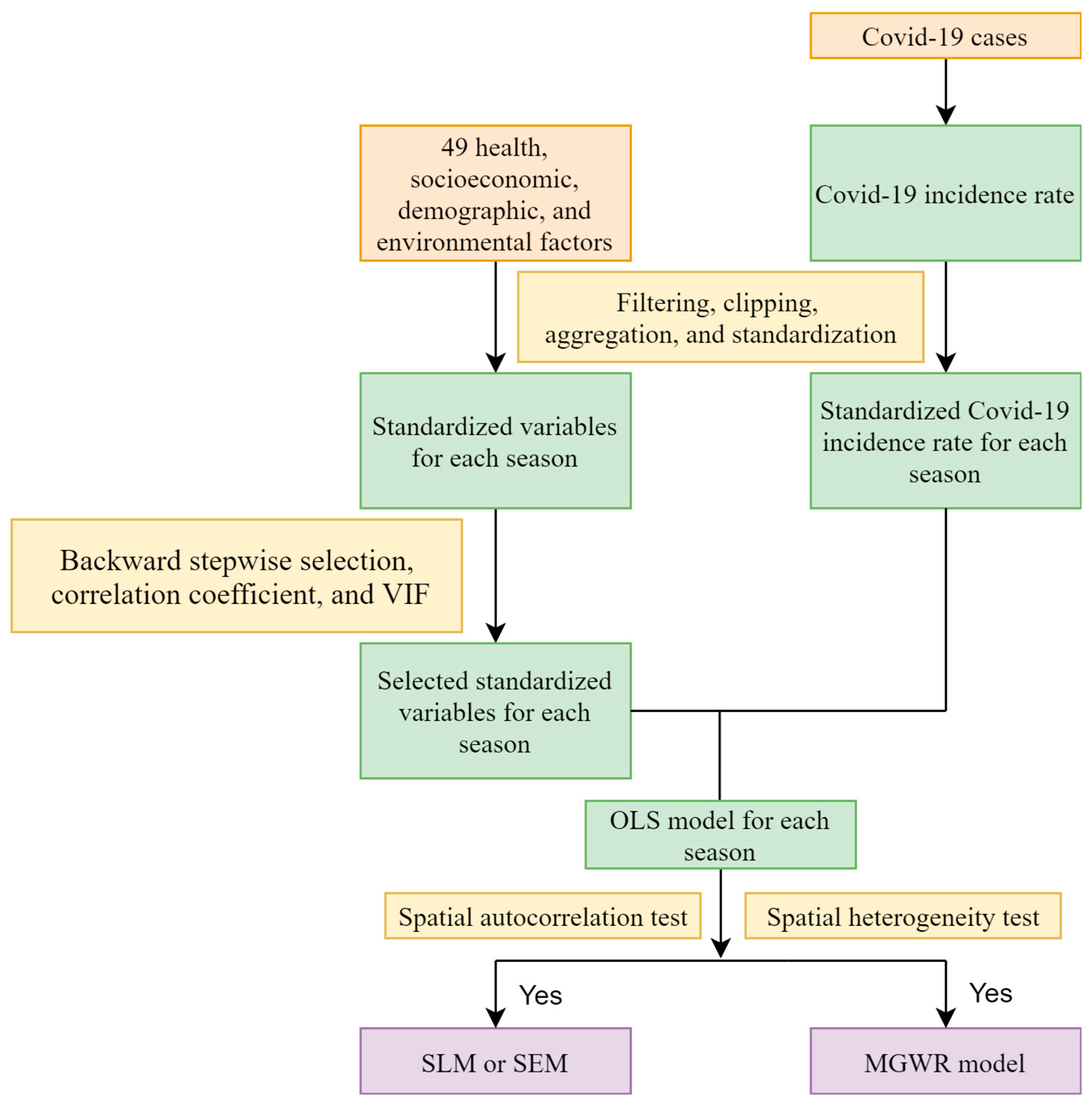
3.2.1. Performance of OLS, SLM, SEM, and MGWR

Table 5. Coefficients of each health, socioeconomic, demographic, and environmental factor from the OLS, SLM, SEM, and MGWR models for each season from 2020 to 2021.

		Coefficient
		OLS	SLM	SEM	MGWR
					Mean	Min	Max
2020 MAM	Intercept	0.00	0.00	0.00	−0.01	−0.02	−0.01
	Adult obesity	0.31 ***	0.31 ***	0.31 ***	0.32	0.28	0.36
	Access to exercise	0.19 **	0.19 **	0.20 **	0.20	0.16	0.23
	Mental distress	−0.39 ***	−0.39 ***	−0.39 ***	−0.39	−0.43	−0.36
	Income inequality	−0.21 **	−0.21 **	−0.20 **	−0.20	−0.22	−0.18
	% of persons in group quarters	0.78 ***	0.78 ***	0.79 ***	0.68	0.19	1.03
	% of persons below 18 years	0.24 **	0.24 **	0.26 ***	0.27	0.25	0.29
	%of native	0.22 **	0.22 **	0.22 **	0.21	0.19	0.24
	% of rural	0.49 ***	0.49 ***	0.51 ***	0.47	0.46	0.48
	Air pollution	−0.22 **	−0.22 ***	−0.22 ***	−0.22	−0.23	−0.21
	Humidity	−0.30 **	−0.30 ***	−0.30 ***	−0.28	−0.30	−0.25
	Temperature	0.41 ***	0.41 ***	0.42 ***	0.42	0.41	0.43
2020 JJA	Intercept	0.00	0.00	0.00	−0.05	−0.06	−0.03
	Diabetes	−0.29 ***	−0.29 ***	−0.30 ***	−0.25	−0.54	−0.03
	Children in poverty	0.34 ***	0.34 ***	0.38 ***	0.25	0.23	0.28
	Income inequality	0.21 **	0.22 **	0.20 **	0.18	−0.01	0.42
	% of persons in group quarters	0.36 ***	0.35 ***	0.34 ***	0.34	0.32	0.37
	% of Hispanic	0.47 ***	0.47 ***	0.49 ***	0.44	0.41	0.46
	Humidity	−0.20 **	−0.20 **	−0.18 ***	−0.15	−0.18	−0.11
2020 SON	Intercept	0.00	0.00	−0.01	−0.05	−0.26	0.31
	Adult obesity	0.26 **	0.19 **	0.17 *	0.16	0.11	0.20
	% of persons in group quarters	0.48 ***	0.48 ***	0.46 ***	0.65	0.23	1.53
	% of non-Hispanic	−0.41 ***	−0.30 ***	−0.19	−0.32	−0.58	−0.13
	Wind	0.32 ***	0.16 *	0.16	0.32	0.17	0.58
2020 DJF	Intercept	0.00	0.00	0.00	0.08	0.05	0.11
	Mental distress	0.19 *	0.16	0.20 *	0.17	0.16	0.19
	Diabetes	0.30 ***	0.29 ***	0.29 ***	0.34	0.14	0.40
	% of 18+ persons with at least one dose	0.35 ***	0.32 ***	0.34 ***	0.30	0.18	0.49
	% of 65 and older	−0.44 ***	−0.39 ***	−0.42 ***	−0.36	−0.70	0.13
2021 MAM	Intercept	0.00	0.00	0.00	−0.01	−0.05	0.04
	% of Asian	−0.20 *	−0.18	−0.19	−0.22	−0.27	−0.18
	% of rural	−0.48 ***	−0.46 ***	−0.48 ***	−0.47	−0.51	−0.42
2021 JJA	Intercept	0.00	−0.02	−0.02	0.08	−0.30	0.33
	Poor health	−0.22 *	−0.15	−0.20	−0.20	−0.56	0.06
	Access to exercise	−0.31 ***	−0.29 ***	−0.30 ***	−0.33	−0.36	−0.29
	Diabetes	0.29 ***	0.32 ***	0.32 ***	0.30	0.26	0.34
	Mask	0.23 **	0.20 **	0.22 **	0.27	0.16	0.34
	% of 65+ persons with at least one dose	0.20 **	0.22 **	0.24 ***	0.20	0.18	0.21
	Unemployment	−0.27 **	−0.28 ***	−0.29 ***	−0.30	−0.39	−0.18
	% of non-Hispanic	−0.34 ***	−0.28 **	−0.25 *	−0.26	−0.30	−0.23
	Humidity	−0.23 **	−0.14	−0.19	−0.14	−0.27	−0.05
2021 SON	Intercept	0.00	0.00	0.00	−0.14	−0.15	−0.13
	Diabetes	0.21 **	0.19 ***	0.20 **	0.19	0.15	0.23
	% of persons with at least one dose	−0.24 ***	−0.18 **	−0.18 **	−0.18	−0.45	0.03
	Children in poverty	0.49 ***	0.43 ***	0.45 ***	0.49	0.48	0.52
	Inadequate facilities in house	−0.20 **	−0.19 **	−0.18 **	−0.19	−0.21	−0.17
	% of persons below 18 years	0.41 ***	0.36 ***	0.35 ***	0.36	0.32	0.42
	% of Hispanic	0.32 ***	0.24 ***	0.29 ***	0.30	0.29	0.31
	% of non-Hispanic White	0.67 ***	0.55 ***	0.62 ***	0.69	0.67	0.72
	Humidity	−0.31 ***	−0.17 *	−0.32 ***	−0.27	−0.49	0.05
2021 DJF	Intercept	0.00	0.00	0.00	0.09	−0.26	0.37
	% of persons with at least one dose	0.41 ***	0.37 ***	0.41 ***	0.41	0.39	0.43
	% of 65 and older	−0.64 ***	−0.57 ***	−0.61 ***	−0.60	−0.60	−0.57
	% of Asian	−0.53 ***	−0.44 ***	−0.46 ***	−0.39	−0.45	−0.14
	% of native Hawaiian	−0.22 **	−0.19 **	−0.19 **	−0.17	−0.26	−0.07
	Humidity	−0.34 ***	−0.31 ***	−0.30 ***	−0.26	−0.35	−0.15
	Wind	0.17 **	0.09	0.17 *	0.13	0.10	0.16

*, **, and *** denote the 10%, 5%, and 1% significant levels.

shows the coefficients of the health, socioeconomic, demographic, and environmental factors derived from the OLS, SLM, SEM, and MGWR models, respectively.

Table 6. Performances of the OLS, SLM, SEM, and MGWR models for each season from 2020 to 2021.

		Breusch–Pagan Test	R-Squared	Adjusted R-Squared	AIC	AICc	Moran’s I for Residual
2020 MAM	OLS	207.06 ***	0.72	0.68	140.24	148.21	0.04
	SLM	207.06 ***	0.72		142.24		0.03
	SEM	204.53 ***	0.73		140.02		0.00
	MGWR		0.82	0.77		128.01	0.00
2020 JJA	OLS	113.11 ***	0.56	0.52	165.44	169.62	−0.09
	SLM	110.21 ***	0.56		167.33		−0.10
	SEM	90.56 ***	0.59		161.93		−0.01
	MGWR		0.64	0.57		167.50	−0.08
2020 SON	OLS	16.96 ***	0.37	0.34	188.06	191.29	0.20 ***
	SLM	20.17 ***	0.50		177.44		−0.02
	SEM	22.10 ***	0.49		178.17		0.01
	MGWR		0.58	0.52		172.64	0.11 *
2020 DJF	OLS	0.82	0.40	0.37	184.59	187.83	0.14 **
	SLM	1.72	0.43		183.99		0.02
	SEM	1.91	0.43		181.93		0.00
	MGWR		0.53	0.46		181.97	0.07
2021 MAM	OLS	1.04	0.19	0.17	202.79	205.36	0.05
	SLM	0.96	0.20		204.34		0.02
	SEM	1.07	0.20		202.27		0.01
	MGWR		0.21	0.16		206.05	0.05
2021 JJA	OLS	10.59	0.45	0.38	186.19	191.63	0.19 ***
	SLM	11.32	0.52		181.28		0.02
	SEM	8.3	0.53		178.58		0.00
	MGWR		0.62	0.53		180.26	0.06
2021 SON	OLS	5.03	0.62	0.57	159.10	164.53	0.12 **
	SLM	4.33	0.67		152.43		−0.09
	SEM	5.17	0.64		156.61		−0.01
	MGWR		0.69	0.62		160.78	0.04
2021 DJF	OLS	1.48	0.59	0.55	160.05	164.24	0.03
	SLM	1.54	0.61		158.76		−0.05
	SEM	1.42	0.59		159.72		−0.01
	MGWR		0.67	0.61		157.68	−0.05

*, **, and *** denote the 10%, 5%, and 1% significant levels.

shows their performances. Note, the adjusted R-squared value and AICc were not reported by GeoDa for both SLM and SEM, and ArcGIS Pro did not report the Breusch–Pagan test and AIC for MGWR.

The adjusted R-squared value is highest for 2020 MAM (0.68), indicating our selected independent variables could explain 68% of the variation in the COVID-19 incidence rate in the OLS model, whereas the OLS model performed the worst for 2021 MAM, and the selected variables only could explain 17% of the variation in the COVID-19 incidence rate. This is confirmed by the AICc values, ranging from 148.21 for 2020 MAM to 205.36 for 2021 MAM (Table 6). Nevertheless, all OLS models are statistically significant at the 5% level, indicating the reliability of the models.

The Moran’s I values of the OLS residuals for 2020 SON, 2020 DJF, 2021 JJA, and 2021 SON are statistically significant (Table 6) at the 10% level, indicating that there is spatial autocorrelation in the residuals. This highlights that the OLS approach is not the best approach for modeling the COVID-19 incidence rate in these seasons. Spatial autocorrelation regression modeling (i.e., SLM and SEM) is necessary to improve the performance. Compared to the OLS models, the R-squared values for 2020 SON, 2020 DJF, 2021 JJA, and 2021 SON increase from 0.37 to 0.50 (0.49), 0.40 to 0.43 (0.43), 0.45 to 0.52 (0.53), and 0.62 to 0.67 (0.64) for SLM (SEM), respectively. Correspondingly, the AIC values of the OLS models for 2020 SON, 2020 DJF, 2021 JJA, and 2021 SON reduce from 188.06 to 177.44 (178.17), 184.59 to 183.99 (181.93), 186.19 to 181.28 (178.58), 159.10 to 152.43 (156.61) for SLM (SEM), respectively. Moreover, the Moran’s I values derived from SLM and SEM for those seasons are statistically insignificant (Table 6). All this indicates the effectiveness of SLM and SEM. For 2020 SON and 2021 SON, SLM performs a little better compared to SEM (Table 6). This is consistent with the results of the LM-lag and LM-error tests, which denot that the LM-lag and robust LM-lag tests are statistically significant for 2020 SON and 2021 SON, while the LM-error test and robust LM-error test are insignificant for 2020 SON and 2021 SON, respectively (Table A3). This implies that the SLM is more appropriate for these two seasons, although their differences are minor (Table 5 and Table 6).

For the residuals without spatial autocorrelation (i.e., 2020 MAM, 2020 JJA, 2021 MAM, and 2021 DJF), we also built the SLM and SEM for comparison purposes. As expected, the performances of the SLM and SEM and OLS are similar (Table 6). Consistently, the coefficients for different factors also show similar values (Table 5).

The Breusch–Panga tests indicate that there is spatial heterogeneity in the residuals of the OLS models for 2020 MAM, 2020 JJA, and 2020 SON (Table 6). It is necessary to develop MGWR for these seasons. We also still built the models for 2020 DJF, 2021 MAM, 2021 JJA, 2021 SON, and 2021 DJF for comparison purposes and being consistent with the other seasons. The highest local condition number of all the models is 13.5, much smaller than 30, indicating the absence of multicollinearity in the local models. As expected, the adjusted R-squared values of the MGWR models for 2020 MAM (0.77), 2020 JJA (0.57), and 2020 SON (0.52) are higher than that of the OLS models (adjusted R-squared = 0.68, 0.52, and 0.34, respectively). Consistently, the AICc values of the MGWR models (128.01, 167.50, and 172.64) are lower than that of the OLS models (148.21, 169.62, and 191.29) over the three seasons (Table 6). Although the residuals of the OLS models for the seasons of 2020 DJF, 2021 JJA, 2021 SON, and 2021 DJF do not have spatial heterogeneity, there are varying bandwidths for the independent variables (Table A4), which may improve the performance of MGWR. However, the adjusted R-squared value (0.16) and AICc (206.05) for 2021 MAM of the MGWR model are found to be similar to the OLS model in the same season (adjusted R-squared = 0.17 and AICc = 205.36) (Table 6). This is within our expectations, as the residuals of the OLS model for the season are randomly distributed, and the bandwidths are all global values for all independent variables (Table A4).

Collectively, the MGWR models outperform OLS, SLM, and SLM (Table 6). The coefficients for each independent variable for each season have consistent signs for all models (Table 5), and the magnitudes of the coefficients for most of the OLS, SLM, and SEM models are within the range of the MGWR models (Table 5). Thus, in the following discussion, we focus on the MGWR results.

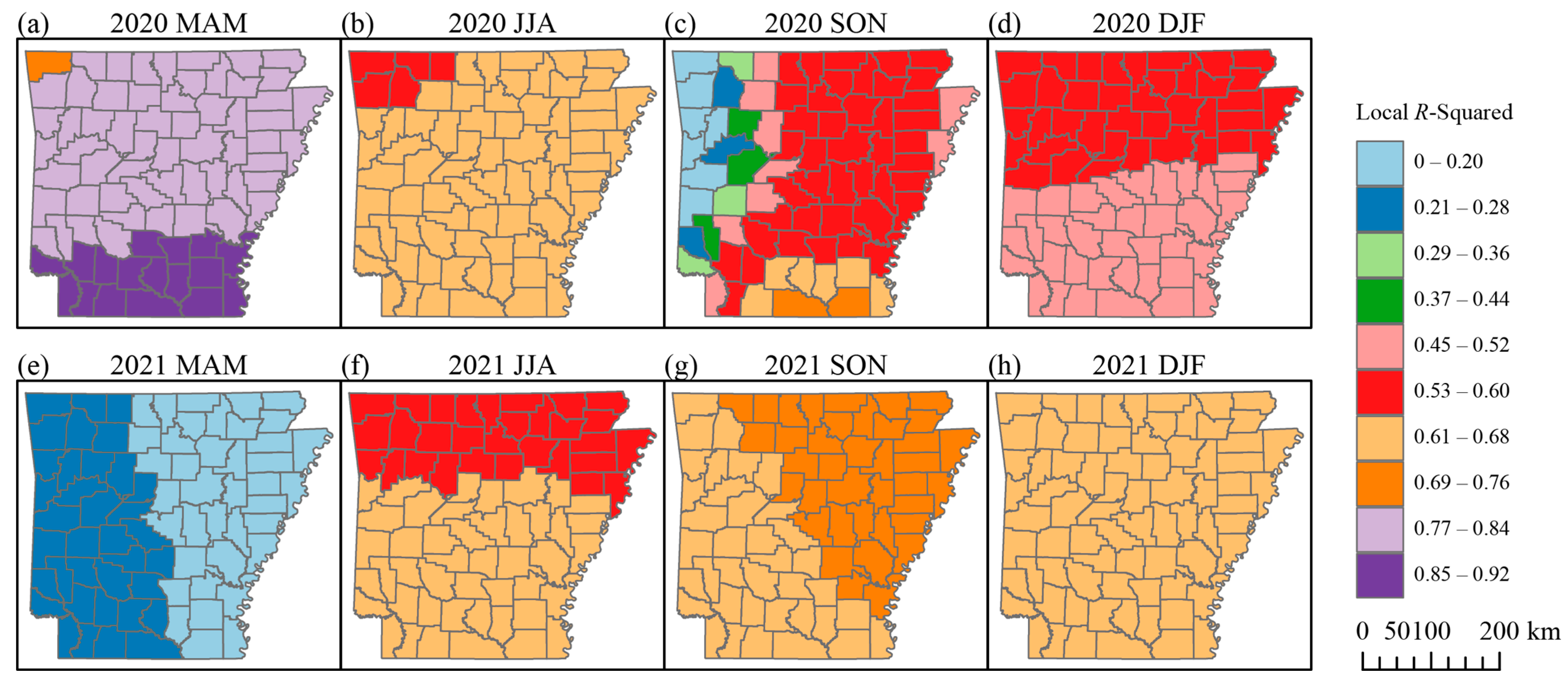
Figure 4 shows the local R-squared values of the MGWR models for each county in each season. Some counties in some seasons have low R-squared values (e.g., R-squared value <0.2 in Benton County in 2020 SON) (Figure 4c). Interestingly, the relatively poor performances of the MGWR models dominate in 2021 MAM (Figure 4e). This may denote that other explanatory variables (e.g., running water [21]) need to be considered in those regions during 2021 MAM. Nevertheless, in most counties and seasons, the local R-squared values of the MGWR models are larger than 0.5 (Figure 4), indicating that our models could capture more than 50% of the variability in the standardized COVID-19 case rate. This implies the relative reliability of MGWR in modeling the COVID-19 rate.

3.2.2. Associations of COVID-19 with Health Factors

Figure 5, Figure 6, Figure 7 and Figure 8 present the spatiotemporal impacts of different health, socioeconomic, demographic, and environmental variables on COVID-19 at the Arkansas county level during all seasons from 2020 to 2021. In general, the associations of the variables from the four categories with COVID-19 vary across space and time.

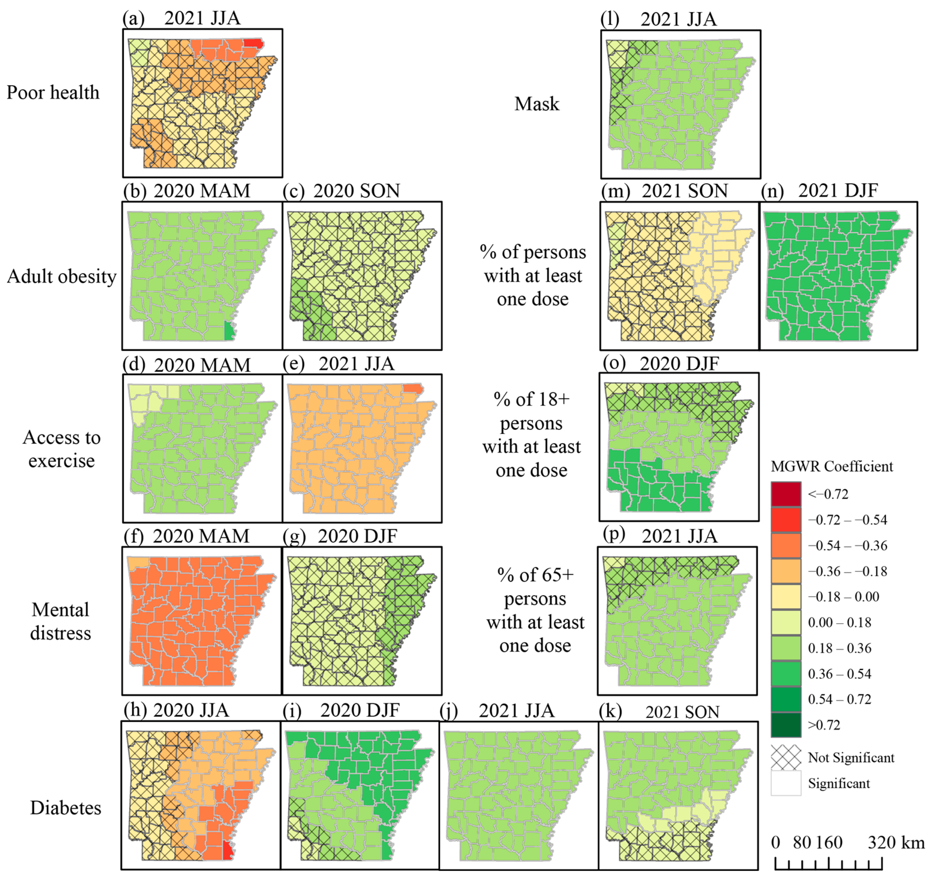
The associations of poor health with COVID-19 are insignificant at the 5% level in most of the counties in Arkansas in the summer of 2021, excepting a few counties in Northern Arkansas, with coefficients ranging from −0.72 to −0.36 (Figure 5a). The significant negative impacts of poor health on COVID-19 may be attributed to people’s preferences to stay at home given the fear of COVID-19 [66], thus reducing the risk of exposure. This may also be the potential reason for the significantly negative associations (coefficients ranging from −0.54 to −0.18) of mental distress with COVID-19 during spring 2020 (Figure 5f).

Adult obesity has significantly positive associations with COVID-19 in all counties during spring 2020, with the highest coefficients (0.36–0.54) in Chicot County (Figure 5b), indicating that people with obesity are vulnerable to COVID-19. Such positive associations persist during fall 2020; however, the effects are not statistically significant at the 5% level (Figure 5c). This finding is consistent with previous studies [67]. Mohammad et al. [68] stated that obesity could weaken the immune system and, therefore, make the host vulnerable to infectious diseases such as COVID-19. Further, Sawadogo et al. [69] demonstrated that people with obesity were at increased risk of both COVID-19-related hospitalizations and death.

The access to exercise shows both significantly negative (coefficients from −0.54 to −0.18) and positive (coefficients from 0.0 to 0.36) associations with COVID-19 during spring 2020 (Figure 5d) and summer 2021 (Figure 5e), respectively. Regular exercise has been shown to improve human immune regulation [70], which may reduce the risk of COVID-19 infection. Yet, exercising may increase the risk of exposure to the virus, especially without social distancing [71]. Arkansas has reopened gyms and fitness centers since 4 May 2020 [72]. As such, people may resume their exercise routines in gyms or fitness centers, which may increase exposure to COVID-19 in a confined environment. However, during the summer, people prefer to exercise outdoors, increasing their contact distance and thus reducing the possibility of COVID-19 infection.

Diabetes shows positive associations with COVID-19 in all counties for winter 2020 (Figure 5i), summer 2021 (Figure 5j), and fall 2021 (Figure 5k), with coefficients ranging from 0 to 0.54, although some counties in Southern Arkansas have insignificant associations (Figure 5i,k)). This is in line with Leon-Abarca et al. [73], who claimed that people with diabetes had a higher probability of being infected after analyzing the cases of more than 1 million Mexican patients. In addition, the positive impacts of diabetes on COVID-19 show spatial variations, with the strongest impacts in Northeastern Arkansas during the winter of 2020 (Figure 5i), while the reason is not clear. Complicating this finding is that diabetes significantly negatively associates with COVID-19 in the eastern part of Arkansas during the summer in 2020 (Figure 5h), with the effects decreasing from the southeastern part (coefficients ranging from −0.72 to −0.54) to northwestern part (coefficients ranging from −0.36 to −0.18). The reasons for the significantly negative associations remain unclear. It may be related to the drugs used by some Type 2 diabetics, as Nyland et al. [74] identified that glucagon-like peptide-1 receptor (GLP-1R) agonists, which have anti-inflammatory effects, were associated with reductions in COVID-19 complications. The stronger negative effects in the southeastern part are probably related to the relatively higher number of people receiving diabetes treatment in this region [75].

As expected, the % of persons with at least one dose shows significantly negative associations with COVID-19 in Eastern Arkansas during fall 2021 (Figure 5m), with coefficients ranging from −0.18 to 0. Moghadas et al. [76] found that vaccination reduced the overall COVID-19 attack rate from 9.0% (without vaccination) to 4.5%. However, vaccination does not always perform as an effective prevention for COVID-19, as stated in Brüssow and Zuber [77]. The % of persons with at least one dose, % of 18+ persons with at least one dose, and % of 65+ persons with at least one dose have significantly positive relationships with COVID-19 during the winter 2020 and 2021 and summer 2021 (Figure 5n–p). This may be due to the fact that people with vaccinations are more likely to break social distances and reduce their willingness to stay at home [78]. Such a reason may also explain the significantly positive associations of masks with COVID-19 during summer 2021 in most Arkansas counties (Figure 5l). The contrasting effects of the % of persons with at least one dose on COVID-19 during fall 2021 (Figure 5m) and winter 2021 (Figure 5n) may be because of changes in people’s perceptions. COVID-19 in fall 2021 was at a low level in Arkansas, which may have led people to change their perception of COVID-19 from severe to weak. Therefore, people may lose their COVID-19 practices (e.g., keeping social distance), resulting in increased infections. There is a spatial variation of the impacts of the % of 18+ persons with at least one dose on COVID-19, with the largest magnitudes in Southern Arkansas, followed by Central Arkansas, in the winter 2020 (Figure 5o). Such variations may be related to the requirement of wearing masks in several universities in Central Arkansas.

Figure 5. Spatial impacts of health variables on the COVID-19 rate derived from a multiscale geographically weighted regression model in each county in Arkansas, US from 2020 to 2021. The unhatched regions indicate a 5% significance level. (MAM: March–April–May; JJA: June–July–August; SON: September–October–November; DJF: December–January–February).

Figure 5. Spatial impacts of health variables on the COVID-19 rate derived from a multiscale geographically weighted regression model in each county in Arkansas, US from 2020 to 2021. The unhatched regions indicate a 5% significance level. (MAM: March–April–May; JJA: June–July–August; SON: September–October–November; DJF: December–January–February).

3.2.3. Associations of COVID-19 with Socioeconomic Factors

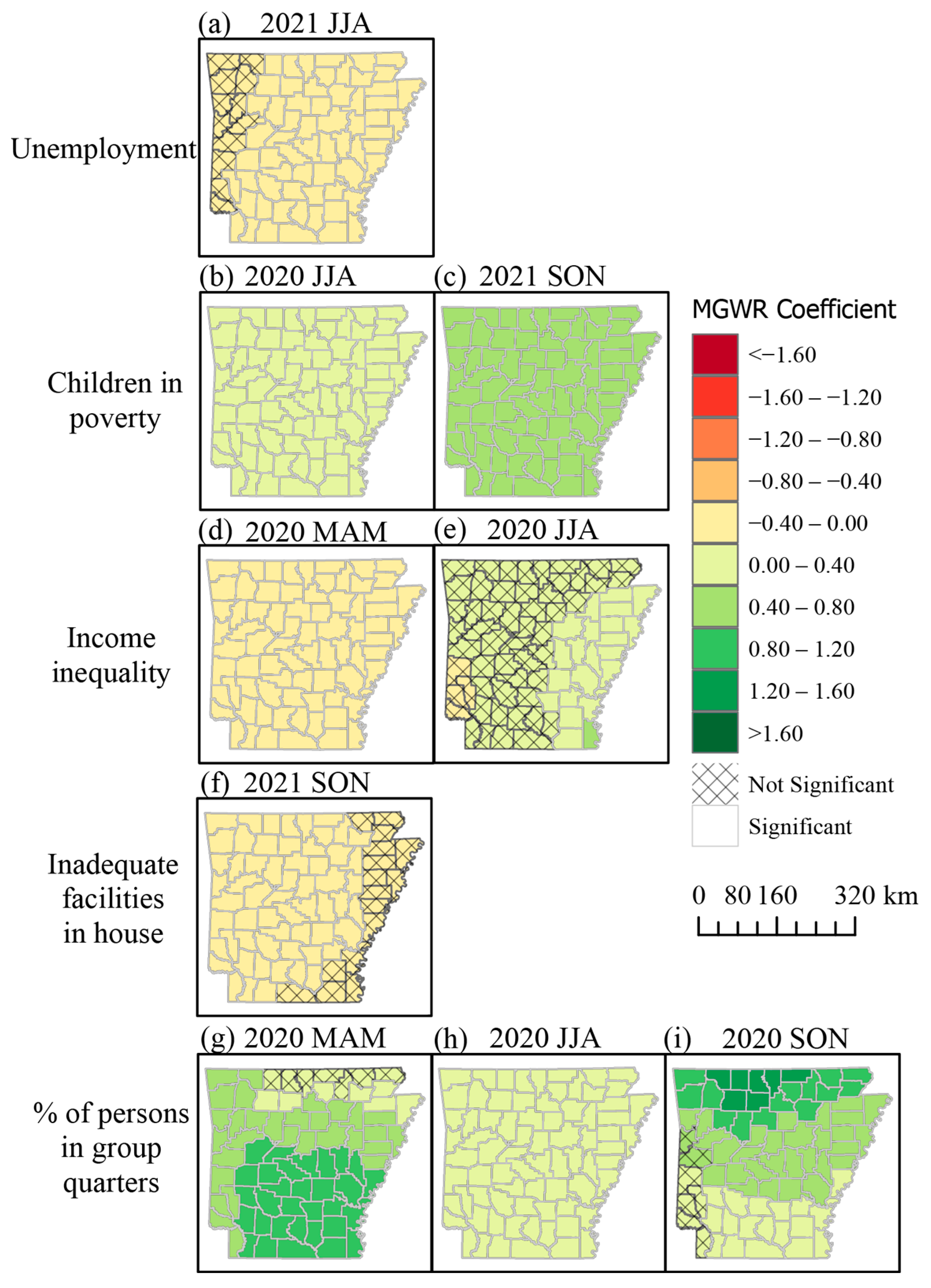
The coefficients of children in poverty with COVID-19 range from 0 to 0.40 in the summer 2020 (Figure 6b) and from 0.40 to 0.80 in the fall 2021 (Figure 6c). Children living in poverty are more likely to experience poor nutrition and live in overcrowded and damp housing and are less likely to have access to green spaces for exercise and less likely to be vaccinated [79]. Thus, they are more vulnerable to catching infectious diseases such as COVID-19.

Consistent with previous studies, income inequality has divergent influences on COVID-19. It has significantly negative effects on the COVID-19 levels in all counties during the spring 2020 (Figure 6d), with the magnitudes ranging from -0.40 to 0, but significantly positive effects (coefficients ranging from 0 to 0.80) on the COVID-19 levels in Eastern Arkansas during the summer 2020 (Figure 6e). Gong and Zhao [80] found that richer people were more mobile and more easily exposed to infection, bringing the virus into their neighborhoods. Oppositely, Demenech et al. [81] found that COVID-19 incidence and mortality increased more pronouncedly among those with greater economic inequality in Brazilian Federative Units. The different signs of impacts of income inequality on COVID-19 may be due to the fact that richer people are more able to work remotely after recognizing the severity of COVID-19, while poorer people, such as the farmers in Eastern Arkansas, have to go outside to make money [1]. This leads to increased COVID-19 infections.

Unlike Ahmad et al. (2020), who found that poor housing conditions induced higher COVID-19 incidence [82], our results show that inadequate facilities significantly negatively affects the COVID-19 levels in most of the counties in Arkansas during the fall 2021 (Figure 6f). This is probably related to the behavior change that households without a kitchen may directly order ready-to-eat food without visiting the grocery stores because of the fear of COVID-19 [83], thus reducing the infection risk.

In general, the % of persons in group quarters has a significantly positive relationship with the COVID-19 levels (Figure 6g–i), with coefficients ranging from 1.20 to 1.60 in Northern-Central Arkansas during the fall 2020 (Figure 6i) to 0 to 0.40 in all of Arkansas during the summer 2020 (Figure 6h). People living in group quarters (e.g., nursing homes, homeless shelters, dormitories, and prisons) usually share space and facilities (e.g., bathrooms). Thus, such positive relationships are anticipated, as the COVID-19 virus spreads mainly between people who are in close contact with each other [84]. The impacts of the % of persons in group quarters on COVID-19 are strongest in Southern Arkansas, followed by the northern and western parts in the spring 2020 (Figure 6g), while the strongest impacts show in Northern-Central Arkansas, followed by the central and southern parts in the fall 2020 (Figure 6i). These variations may be related to interactions with other factors (Table 5), which needs to be further examined.

Surprisingly, we found negative associations of being unemployment (Figure 6a) with COVID-19 levels. One possible reason is that unemployment people are unlikely to test for COVID-19 given their financial burdens [85], leading to many unreported cases among these groups.

Figure 6. Spatial impacts of the socioeconomic variables on the COVID-19 rate derived from the multiscale geographically weighted regression model on COVID-19 in each county in Arkansas, US from 2020 to 2021. The unhatched regions indicate a 5% significance level. (MAM: March–April–May; JJA: June–July–August; SON: September–October–November; DJF: December–January–February).

Figure 6. Spatial impacts of the socioeconomic variables on the COVID-19 rate derived from the multiscale geographically weighted regression model on COVID-19 in each county in Arkansas, US from 2020 to 2021. The unhatched regions indicate a 5% significance level. (MAM: March–April–May; JJA: June–July–August; SON: September–October–November; DJF: December–January–February).

3.2.4. Associations of COVID-19 with Demographic Factors

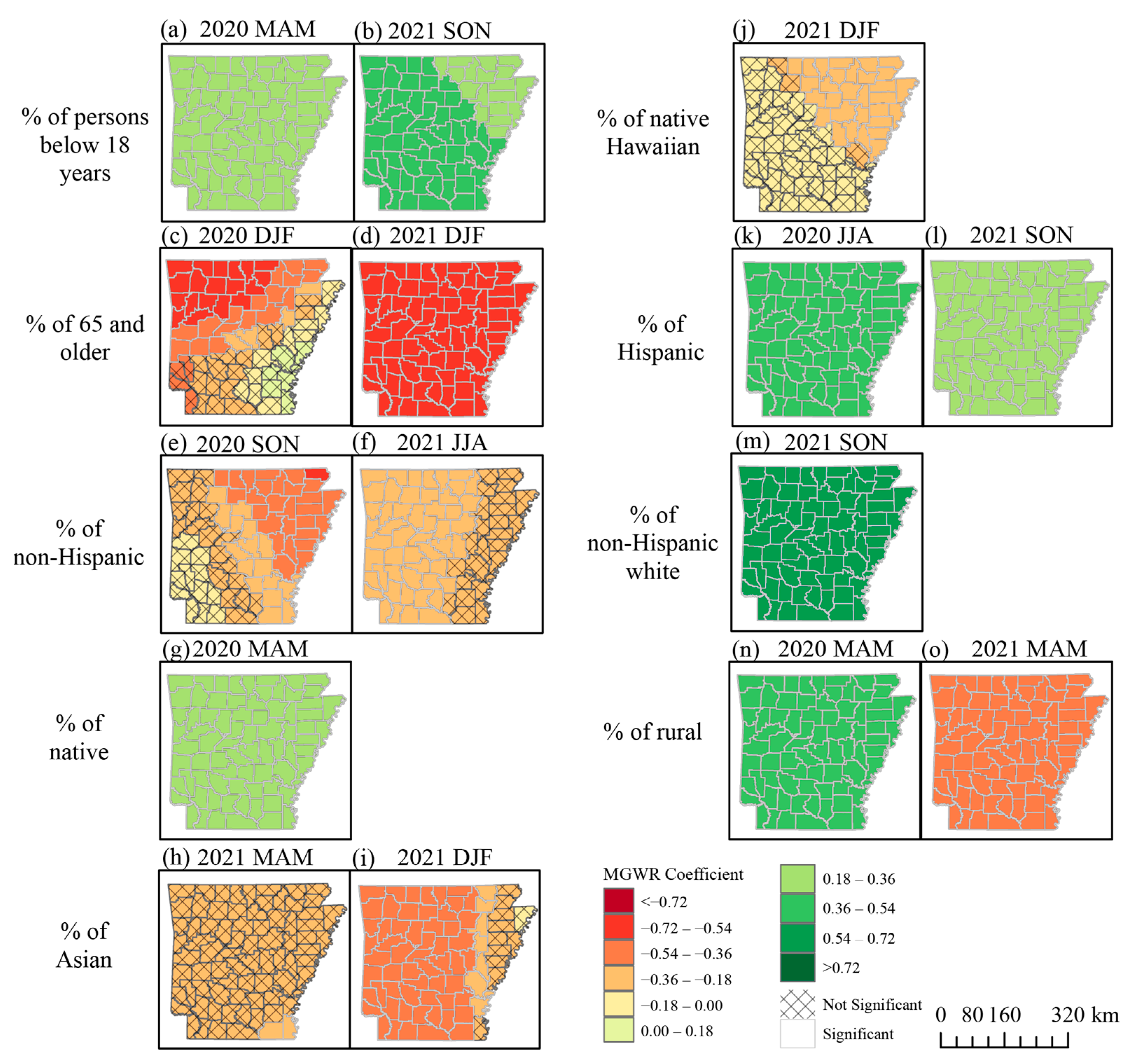
For demographic impacts, there are significantly positive relationships of the % of persons below 18 years (Figure 7a,b), % of native (Figure 7g), % of Hispanic (Figure 7k,l), and % of non-Hispanic White (Figure 7m) with COVID-19 in all counties in Arkansas during different seasons, with coefficients ranging from 0.18 to 0.72. These findings are consistent with previous research. According to the CDC [86], older teens, ages 16 and 17, face the highest rate of weekly cases. This is reinforced by Rumain et al. [87], who concluded that the prevalence of COVID-19 for adolescents (10–19) was significantly greater than that for older adults. McLernon [88] reported that COVID-19 cases, mortality, and case fatality incidences were 2.2, 3.8, and 1.7 times higher for Native Americans compared with White people in Montana. Further, Weeks [89] stated that the American Indian and Alaska Native communities have been experiencing some of the highest rates of COVID-19 in the United States based on the maps generated by The John’s Hopkins Coronavirus Resource Center. As Hispanics or Latinos are heavily represented in the service industry, they were 1.5 times more likely to contact COVID-19 than their non-Hispanic White counterparts, as well as 1.9 times more likely to be hospitalized from COVID-19 and 1.8 times more likely to die from COVID-19 [90]. The White population has a relatively low vaccination rate (only 50% of the population are fully vaccinated), leading to a high risk of COVID-19 [91].

The % of 65 and older has a significantly negative impact on the COVID-19 levels during the winter 2020 and 2021 (Figure 7c,d), with coefficients ranging from −0.72 to −0.18. Due to the severe illness of COVID-19 in older people, the CDC has suggested giving the top priority to more senior people to get the vaccine [92]. As such, more than 95% of 65 to 74 years old people in the U.S. received at least one dose of the vaccine [91], which thereby may reduce the total COVID-19 burden. In addition, the % of 65 and older shows the strongest negative impacts in Northwestern Arkansas, followed by a belt stretching from the northeastern to southwestern parts in the winter 2020 (Figure 7c). Such variations need to be further explored.

Unlike Native Americans and Hispanics, the % of Asians and % of Native Hawaiians show significantly negative relationships with the COVID-19 levels in Southeastern Arkansas in the spring 2021 (Figure 7h) and Western and Northeastern Arkansas in the winter 2021 (Figure 7i,j). The magnitudes of the relationships range from −0.54 to −0.18. Asians and Native Hawaiian/Pacific Islanders has high vaccination rates. The vaccination may provide some protection for them from COVID-19 [91].

The % of rural parts has both significantly positive (coefficients ranging from 0.36 to 0.54) and negative (coefficients ranging from −0.54 to −0.36) associations with COVID-19 during the spring 2020 (Figure 7n) and spring 2021 (Figure 7o), respectively. The rural area populations tend to be older, sicker, heavier, poorer, and less vaccinated and have experienced higher COVID-19 incidence and mortality rates [93]. Meanwhile, the population density in rural areas is lower compared to metropolitan areas [94], leading to a reduction in COVID-19 transmission. The different signs of impacts are presumably due to the fact that after getting vaccination and a better education, people in rural areas with a lower population density and more open space are less likely to be infected by COVID-19.

As for the impacts of unemployment impacts on COVID-19, the negative influences of the % of non-Hispanic Blacks on COVID-19 (Figure 7e,f) are presumably because of the hidden COVID-19 cases caused by the inability to test for it, which need to be further explored.

Figure 7. Spatial impacts of demographic variables on the COVID-19 rate derived from a multiscale geographically weighted regression model on COVID-19 in each county in Arkansas, US from 2020 to 2021. The unhatched regions indicate a 5% significance level. (MAM: March–April–May; JJA: June–July–August; SON: September–October–November; DJF: December–January–February).

Figure 7. Spatial impacts of demographic variables on the COVID-19 rate derived from a multiscale geographically weighted regression model on COVID-19 in each county in Arkansas, US from 2020 to 2021. The unhatched regions indicate a 5% significance level. (MAM: March–April–May; JJA: June–July–August; SON: September–October–November; DJF: December–January–February).

3.2.5. Associations of COVID-19 with Climate Factors

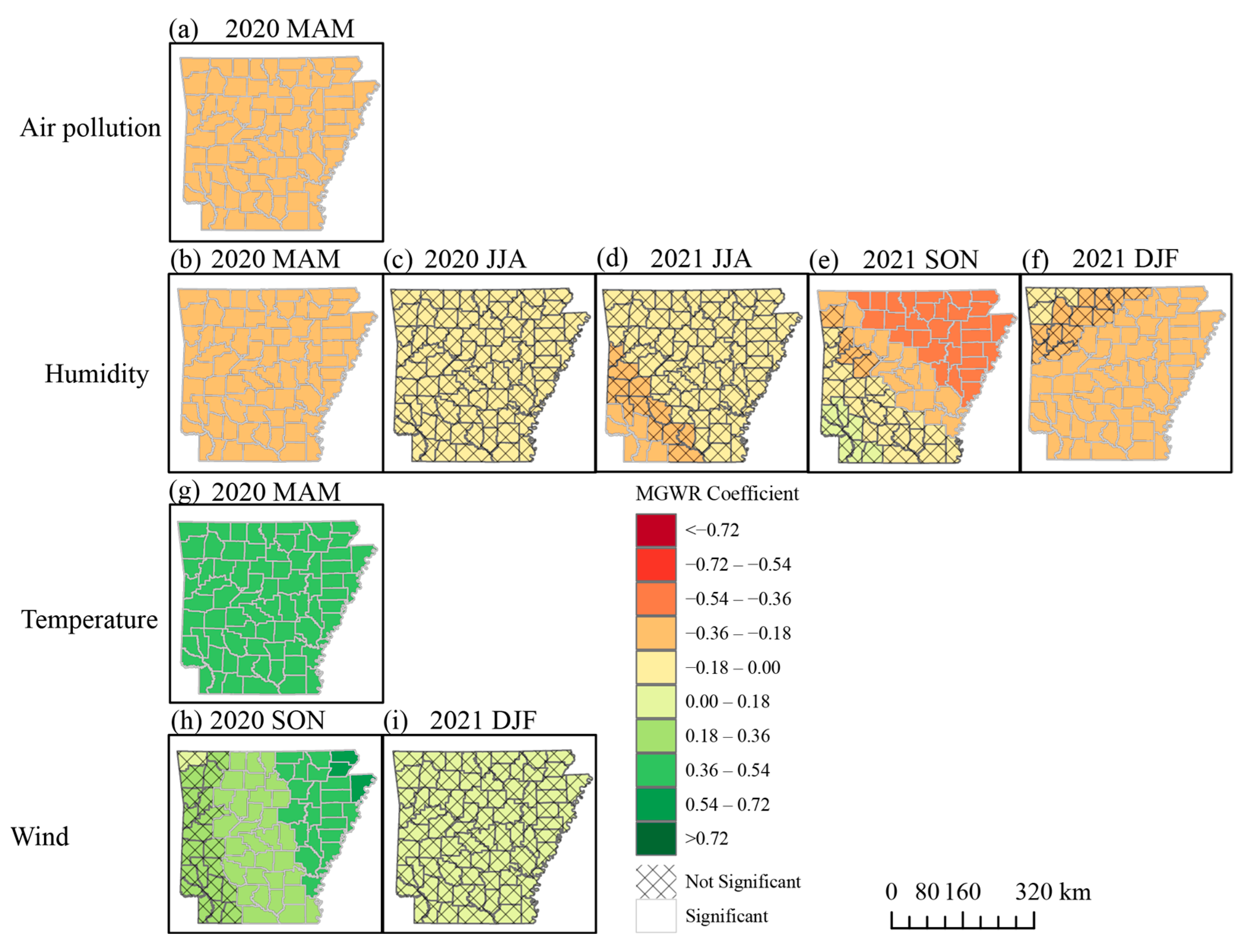
Air pollution has significantly negative effects on COVID-19 in all of Arkansas during the spring 2020 (Figure 8a). This supports the previous study that COVID-19 cases were reduced when the amount of PM_2.5 was above the threshold level, as a higher concentration of PM_2.5 may restrict human mobility [95].

The humidity consistently shows significantly negative effects on the COVID-19 levels in Arkansas during the spring 2020 (Figure 8b), summer 2021 (Figure 8d), fall 2021 (Figure 8e), and winter 2021 (Figure 8f). The effects are the strongest in Northeastern Arkansas during the fall 2021, with coefficients ranging from −0.54 to −0.36. These negative effects have been documented by existing studies. For instance, Ward et al. [96] found that a reduction in the relative humidity of 1% was predicted to be associated with an increase of COVID-19 cases by ~6% in New South Wales, Australia. By reviewing 517 articles, Mecenas et al. [97] concluded that a wet climate appeared to reduce the spread of COVID-19. The impacts of humidity on COVID-19 in the fall 2021 show spatial variations, with the largest magnitudes in Northeastern Arkansas, followed by a belt stretching from the northwestern to southeastern parts (Figure 8e).

The temperature significantly positively influenced the COVID-19 levels (Figure 8g) in Arkansas during the spring of 2020. Menebo et al. [16] stated that people were more prone to outdoor activities when the sun was shining outside and so eventually became exposed to the virus.

The wind also shows significantly positive impacts on COVID-19 during the fall 2020 (Figure 8h). A high wind speed likely circulated any suspended respiratory droplets in the air and thereby increased the possibility of inhalation by people. 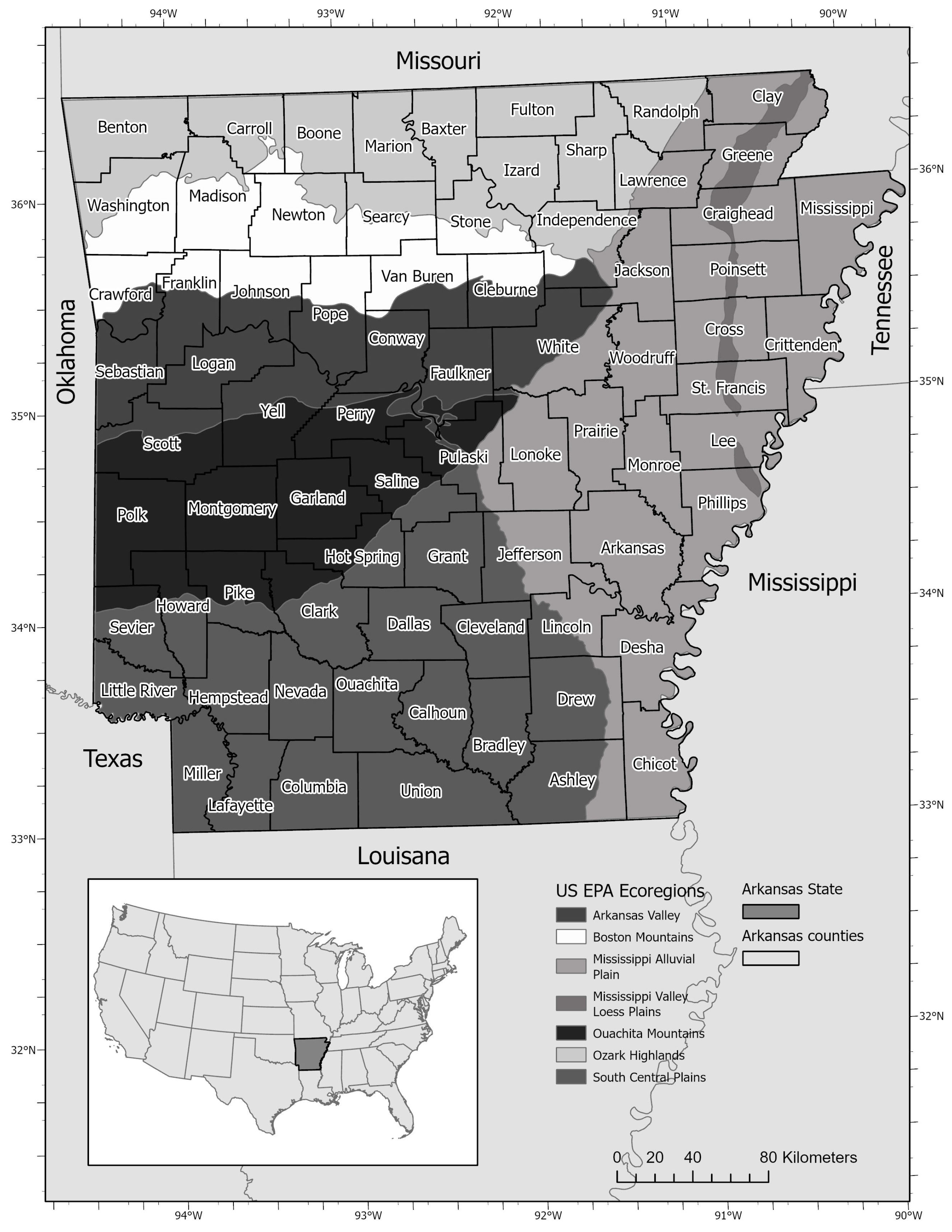The impacts of wind on COVID-19 gradually decrease from Northeastern Arkansas to Southwestern Arkansas (Figure 8h), which is possibly because of the mountainous terrain in Western Arkansas (Figure 1) that blocks the wind to circulate the droplets.

Figure 8. Spatial impacts of climate variables on the COVID-19 rate derived from a geographically weighted regression model on COVID-19 in each county in Arkansas, US from 2020 to 2021. The unhatched regions indicate a 5% significance level. (MAM: March–April–May; JJA: June–July–August; SON: September–October–November; DJF: December–January–February).

Figure 8. Spatial impacts of climate variables on the COVID-19 rate derived from a geographically weighted regression model on COVID-19 in each county in Arkansas, US from 2020 to 2021. The unhatched regions indicate a 5% significance level. (MAM: March–April–May; JJA: June–July–August; SON: September–October–November; DJF: December–January–February).

In summary, different factors contribute to COVID-19 transmission across time. This may be because different variables were involved in the MGWR models in different seasons. For instance, during the spring season in 2020, there were 11 factors from four categories contributing to the COVID-19 rate variation, while, in spring 2021, only two factors from two categories explained the COVID-19 rate variation. Along with different COVID-19 variants (i.e., early variants in winter 2020, Delta in summer 2021, and Omicron in winter 2021), the contributions of driving factors are different. Only diabetes shows consistently positive roles in the spread of both early COVID-19 variants and Delta, while humidity plays consistently negative roles in the spread of both Delta and Omicron.

4. Conclusions

The COVID-19 pandemic continues to affect all aspects of society. Attributing the reasons underlying the pandemic’s spread at the local scale could help policymakers develop more appropriate prevention strategies to combat COVID-19 and protect local people. In this study, we explored the spatiotemporal patterns of COVID-19 in Arkansas using a hot spot analysis. We then applied a multiscale geographically weighted regression model to thoroughly assess how health, socioeconomic, demographic, and environmental factors affected COVID-19 spread in Arkansas counties, covering all seasons from 2020 to 2021.

The results show that COVID-19 dominates Arkansas’ two major cities (Little Rock and Fayetteville). The MGWR models successfully capture the spatial variation of COVID-19 with R² above 0.5 in most counties across different seasons. The MGWR analyses reveal that people with obesity are more likely to be infected by the COVID-19 virus over all of Arkansas, as well as people with diabetes, despite the existence of negative impacts in mid-2020. Thus, targeted interventions (e.g., distribution of personal protective equipment) should be focused on these groups of people. Exercising generates the potential for people to be more protective against COVID-19. However, our study also reveals that access to exercise positively correlates with COVID-19 cases, suggesting that people should be cautious when exercising, especially to avoid presenting in crowded environments. Consistent with the medical theory, this study finds that vaccination can protect people from COVID-19. Yet, we also reveal that vaccination does not always work. We therefore strongly recommend that vaccinated people still practice social distancing or wearing masks.

Children in poverty and % of persons living in group quarters are both prone to COVID-19 infection. We thus suggest the local government pay great attention to these groups of people, such as distributing more nutrients to children in poverty andincreasing the sanitation conditions in the quarters.

Hispanics are also at risk of COVID-19, largely due to their work sectors (i.e., service industry). Therefore, social distancing and mask are recommended in restaurants or supermarkets, etc. More COVID-19 education (e.g., frequently washing hands and avoiding crowd activities) may be required to reduce the COVID-19 rates in teenagers. We also find that White populations are positively associated with the COVID-19 incidence rate, which may be due to the relative low vaccination rate. Thus, promoting the vaccination rate is still needed for this group of people.

Increased temperature and wind in Arkansas failed to reduce the virus’s spread. Thus, we suggest that local people should keep general COVID-19 practices in hot or windy seasons. Humidity shows consistently negative associations with the COVID-19 incidence rate in Arkansas; we thus suggest increasing humidity (e.g., using a humidifier in the bedroom) in residential units.

Our study provides a scientific basis for preventing COVID-19 spread at the county level in Arkansas, US. The methodology used in this study can be applied to any other geographic region that experiences COVID-19 or similar infectious diseases. Yet, there are several limitations in our study. First, there may be other factors influencing COVID-19, such as human mobility and immunity in previous seasons. Future studies need to consider such factors. Second, we find the negative relationships of the unemployment and % of non-Hispanic Black populations with COVID-19, which may be due to hidden COVID-19 cases because of the inability to test it. More accurate data of COVID-19 cases in these two groups are required to better understand their associations with COVID-19. Third, this study did not consider interactions among different factors and interactions between space and time [98,99], and such sophisticated interaction parameters need to be included in the local spatial or spatiotemporal models to improve their performances. Finally, there are spatial variations in the magnitudes of the effects of different factors on COVID-19. More county-level information, such as education on COVID-19, people’s behavior choices, and local terrain information, is needed to better explain these patterns.

References

1. Huang, X.; Lu, J.; Gao, S.; Wang, S.; Liu, Z.; Wei, H. Staying at Home Is a Privilege: Evidence from Fine-Grained Mobile Phone Location Data in the United States during the COVID-19 Pandemic. Ann. Am. Assoc. Geogr. 2022, 112, 286–305. [Google Scholar] [CrossRef]
2. Huang, X.; Li, Z.; Jiang, Y.; Li, X.; Porter, D. Twitter reveals human mobility dynamics during the COVID-19 pandemic. PLoS ONE 2020, 15, e0241957. [Google Scholar] [CrossRef]
3. Lancaster, E.; Ai, Y.; Lee, J. Socioeconomic Status Associations with Confirmed COVID-19 Cases and SARS-CoV-2 Wastewater Concentrations in Small-Medium Sized Communities. Environ. Res. 2022, 215, 114290. [Google Scholar] [CrossRef] [PubMed]
4. Shereen, M.A.; Khan, S.; Kazmi, A.; Bashir, N.; Siddique, R. COVID-19 infection: Origin, transmission, and characteristics of human coronaviruses. J. Adv. Res. 2020, 24, 91–98. [Google Scholar] [CrossRef] [PubMed]
5. WHO. WHO Coronavirus (COVID-19) Dashboard. Available online: https://covid19.who.int/ (accessed on 7 February 2022).
6. Martins, D.L.; da Silva, I.; Batista, W.V.; de Fatima Andrade, M.; de Freitas, E.D.; Martins, J.A. How socio-economic and atmospheric variables impact COVID-19 and influenza outbreaks in tropical and subtropical regions of Brazil. Environ. Res. 2020, 191, 110184. [Google Scholar] [CrossRef]
7. Diffenbaugh, N.S.; Field, C.B.; Appel, E.A.; Azevedo, I.L.; Baldocchi, D.D.; Burke, M.; Burney, J.A.; Ciais, P.; Davis, S.J.; Fiore, A.M.; et al. The COVID-19 lockdowns: A window into the Earth System. Nat. Rev. Earth Environ. 2020, 1, 470–481. [Google Scholar] [CrossRef]
8. Alam, M.S.; Sultana, R. Influences of climatic and non-climatic factors on COVID-19 outbreak: A review of existing literature. Environ. Chall. 2021, 5, 100255. [Google Scholar] [CrossRef]
9. Guo, M.; Yang, L.; Shen, F.; Zhang, L.; Li, A.; Cai, Y.; Zhou, C. Impact of socio-economic environment and its interaction on the initial spread of COVID-19 in mainland China. Geospat. Health 2022, 17, 1–11. [Google Scholar] [CrossRef]
10. Paraskevis, D.; Kostaki, G.E.; Alygizakis, N.; Thomaidis, N.S.; Cartalis, C.; Tsiodras, S.; Dimopoulos, A.M. A review of the impact ofweather and climate variables to COVID-19: In the absence of public health measures high temperatures cannot probably mitigate outbreaks. Sci. Total Environ. 2020, 768, 144578. [Google Scholar] [CrossRef]
11. Ganslmeier, M.; Furceri, D.; Ostry, J.D. The impact of weather on COVID-19 pandemic. Sci. Rep. 2021, 11, 22027. [Google Scholar] [CrossRef]
12. Rosario, D.K.A.; Mutz, Y.S.; Bernardes, P.C.; Conte-Junior, C.A. Relationship between COVID-19 and weather: Case study in a tropical country. Int. J. Hyg. Environ. Health 2020, 229, 113587. [Google Scholar] [CrossRef] [PubMed]
13. Bashir, M.F.; Ma, B.; Bilal; Komal, B.; Bashir, M.A.; Tan, D.; Bashir, M. Correlation between climate indicators and COVID-19 pandemic in New York, USA. Sci. Total Environ. 2020, 728, 138835. [Google Scholar] [CrossRef] [PubMed]
14. Coskun, H.; Yildirim, N.; Gunduz, S. The spread of COVID-19 virus through population density and wind in Turkey cities Hamit. Sci. Total Environ. 2021, 751, 141663. [Google Scholar] [CrossRef] [PubMed]
15. Fern’andez-Ahúja, J.M.L.; Martínez, J.L.F. Effects of climate variables on the COVID-19 outbreak in Spain. Int. J. Hyg. Environ. Health 2021, 234, 113723. [Google Scholar] [CrossRef]
16. Menebo, M.M. Temperature and precipitation associate with Covid-19 new daily cases: A correlation study between weather and Covid-19 pandemic in Oslo, Norway. Sci. Total Environ. 2020, 737, 139659. [Google Scholar] [CrossRef] [PubMed]
17. Wang, J.; Tang, K.; Feng, K.; Lin, X.; Lv, W.; Chen, K.; Wang, F. Impact of temperature and relative humidity on the transmission of COVID-19: A modelling study in China and the United States. BMJ Open 2021, 11, e043863. [Google Scholar] [CrossRef]
18. Ahmed, J.; Jaman, M.H.; Saha, G.; Ghosh, P. Effect of environmental and socio-economic factors on the spreading of COVID-19 at 70 cities/provinces. Heliyon 2021, 7, e06979. [Google Scholar] [CrossRef]
19. Yang, X.D.; Su, X.Y.; Li, H.L.; Ma, R.F.; Qi, F.J.; Cao, Y.E. Impacts of socio-economic determinants, spatial distance and climate factors on the confirmed cases and deaths of COVID-19 in China. PLoS ONE 2021, 16, e0255229. [Google Scholar] [CrossRef]
20. Rahman, M.; Islam, M.; Shimanto, M.H.; Ferdous, J.; Rahman, A.A.N.S.; Sagor, P.S.; Chowdhury, T. A global analysis on the effect of temperature, socio-economic and environmental factors on the spread and mortality rate of the COVID-19 pandemic. Environ. Dev. Sustain. 2021, 23, 9352–9366. [Google Scholar] [CrossRef]
21. Da Silva, C.F.A.; Silva, M.C.; dos Santos, A.M.; Rudke, A.P.; do Bonfim, C.V.; Portis, G.T.; de Almeida Junior, P.M.; Coutinho, M.B.d.S. Spatial analysis of socio-economic factors and their relationship with the cases of COVID-19 in Pernambuco, Brazil. Trop. Med. Int. Health 2022, 27, 397–407. [Google Scholar] [CrossRef]
22. Tang, J.W.; Caniza, M.A.; DInn, M.; Dwyer, D.E.; Heraud, J.M.; Jennings, L.C.; Kok, J.; Kwok, K.O.; Li, Y.; Loh, T.P.; et al. An exploration of the political, social, economic and cultural factors affecting how different global regions initially reacted to the COVID-19 pandemic. Interface Focus 2022, 12, 20210079. [Google Scholar] [CrossRef] [PubMed]
23. Bashir, M.F.; Ma, B.; Shahzad, L. A brief review of socio-economic and environmental impact of Covid-19. Air Qual. Atmos. Health 2020, 13, 1403–1409. [Google Scholar] [CrossRef] [PubMed]
24. Mena, G.E.; Martinez, P.P.; Mahmud, A.S.; Marquet, P.A.; Buckee, C.O.; Santillana, M. Socioeconomic status determines COVID-19 incidence and related mortality in Santiago, Chile. Science 2021, 372, eabg5298. [Google Scholar] [CrossRef] [PubMed]
25. Igoe, M.; Das, P.; Lenhart, S.; Lloyd, A.L.; Luong, L.; Tian, D.; Lanzas, C.; Odoi, A. Geographic disparities and predictors of COVID-19 hospitalization risks in the St. Louis Area, Missouri (USA). BMC Public Health 2022, 22, 321. [Google Scholar] [CrossRef] [PubMed]
26. Wang, Y.; Tsai, T.C.; Duncan, D.T.; Ji, J.S. Association of city-level walkability, accessibility to biking and public transportation and socio-economic features with COVID-19 infection in Massachusetts, USA: An ecological study. Geospat. Health 2022, 17, 33–42. [Google Scholar] [CrossRef]
27. Ali, T.; Mortula, M.; Sadiq, R. GIS-based vulnerability analysis of the United States to COVID-19 occurrence. J. Risk Res. 2021, 24, 416–431. [Google Scholar] [CrossRef]
28. Luo, Y.; Yan, J.; McClure, S. Distribution of the environmental and socioeconomic risk factors on COVID-19 death rate across continental USA: A spatial nonlinear analysis. Environ. Sci. Pollut. Res. 2021, 28, 6587–6599. [Google Scholar] [CrossRef]
29. Qiu, Y.; Chen, X.; Shi, W. Impacts of social and economic factors on the transmission of coronavirus disease 2019 (COVID-19) in China. J. Popul. Econ. 2020, 33, 1127–1172. [Google Scholar] [CrossRef]
30. Maiti, A.; Zhang, Q.; Sannigrahi, S.; Pramanik, S.; Chakraborti, S.; Cerda, A.; Pilla, F. Exploring spatiotemporal effects of the driving factors on COVID-19 incidences in the contiguous United States. Sustain. Cities Soc. 2021, 68, 102784. [Google Scholar] [CrossRef]
31. Akinwumiju, A.S.; Oluwafemi, O.; Mohammed, Y.D.; Mobolaji, J.W. Geospatial evaluation of COVID-19 mortality: Influence of socio-economic status and underlying health conditions in contiguous USA. Appl. Geogr. 2022, 141, 102671. [Google Scholar] [CrossRef]
32. Almalki, A.; Gokaraju, B.; Acquaah, Y.; Turlapaty, A. Regression Analysis for COVID-19 Infections and Deaths Based on Food Access and Health Issues. Healthcare 2022, 10, 324. [Google Scholar] [CrossRef] [PubMed]
33. Iyanda, A.E.; Boakye, K.A.; Lu, Y.; Oppong, J.R. Racial/Ethnic Heterogeneity and Rural-Urban Disparity of COVID-19 Case Fatality Ratio in the USA: A Negative Binomial and GIS-Based Analysis. J. Racial Ethn. Health Disparities 2022, 9, 708–721. [Google Scholar] [CrossRef] [PubMed]
34. Juhn, Y.J.; Wheeler, P.; Wi, C.-I.; Bublitz, J.; Ryu, E.; Ristagno, E.H.; Patten, C. Role of Geographic Risk Factors in COVID-19 Epidemiology: Longitudinal Geospatial Analysis. Mayo Clin. Proc. Innov. Qual. Outcomes 2021, 5, 916–927. [Google Scholar] [CrossRef] [PubMed]
35. Kandula, S.; Shaman, J. Investigating associations between COVID-19 mortality and population-level health and socioeconomic indicators in the United States: A modeling study. PLoS Med. 2021, 18, e1003693. [Google Scholar] [CrossRef] [PubMed]
36. Lyu, T.; Hair, N.; Yell, N.; Li, Z.; Qiao, S.; Liang, C.; Li, X. Temporal geospatial analysis of covid-19 pre-infection determinants of risk in South Carolina. Int. J. Environ. Res. Public Health 2021, 18, 9673. [Google Scholar] [CrossRef]
37. Mollalo, A.; Rivera, K.M.; Vahedi, B. Artificial neural network modeling of novel coronavirus (COVID-19) incidence rates across the continental United States. Int. J. Environ. Res. Public Health 2020, 17, 4204. [Google Scholar] [CrossRef]
38. Mollalo, A.; Vahedi, B.; Rivera, K.M. GIS-based spatial modeling of COVID-19 incidence rate in the continental United States. Sci. Total Environ. 2020, 728, 138884. [Google Scholar] [CrossRef]
39. Mollalo, A.; Tatar, M. Spatial modeling of covid-19 vaccine hesitancy in the united states. Int. J. Environ. Res. Public Health 2021, 18, 9488. [Google Scholar] [CrossRef]
40. Oluyomi, A.O.; Gunter, S.M.; Leining, L.M.; Murray, K.O.; Amos, C. COVID-19 community incidence and associated neighborhood-level characteristics in Houston, Texas, USA. Int. J. Environ. Res. Public Health 2021, 18, 1495. [Google Scholar] [CrossRef]
41. Tepe, E. The impact of built and socio-economic environment factors on Covid-19 transmission at the ZIP-code level in Florida. J. Environ. Manag. 2023, 326, 116806. [Google Scholar] [CrossRef]
42. Vopham, T.; Weaver, M.D.; Adamkiewicz, G.; Hart, J.E. Social distancing associations with COVID-19 infection and mortality are modified by crowding and socioeconomic status. Int. J. Environ. Res. Public Health 2021, 18, 4680. [Google Scholar] [CrossRef] [PubMed]
43. Whittle, R.S.; Diaz-Artiles, A. An ecological study of socioeconomic predictors in detection of COVID-19 cases across neighborhoods in New York City. BMC Med. 2020, 18, 271. [Google Scholar] [CrossRef] [PubMed]
44. Zhang, C.H.; Schwartz, G.G. Spatial Disparities in Coronavirus Incidence and Mortality in the United States: An Ecological Analysis as of May 2020. J. Rural Health 2020, 36, 433–445. [Google Scholar] [CrossRef] [PubMed]
45. Wang, C.; Li, Z.; Clay Mathews, M.; Praharaj, S.; Karna, B.; Solís, P. The spatial association of social vulnerability with COVID-19 prevalence in the contiguous United States. Int. J. Environ. Health Res. 2022, 32, 1147–1154. [Google Scholar] [CrossRef] [PubMed]
46. Mansour, S.; Abulibdeh, A.; Alahmadi, M.; Al-Said, A.; Al-Said, A.; Watmough, G.; Atkinson, P.M. Spatial Associations between COVID-19 Incidence Rates and Work Sectors: Geospatial Modeling of Infection Patterns among Migrants in Oman. Ann. Am. Assoc. Geogr. 2022, 112, 1974–1993. [Google Scholar] [CrossRef]
47. Comber, A.; Brunsdon, C.; Charlton, M.; Dong, G.; Harris, R.; Lu, B.; Yihe, L.; Murakami, D.; Nakaya, T.; Wang, Y.; et al. A Route Map for Successful Applications of Geographically Weighted Regression. Geogr. Anal. 2022, 55, 1–24. [Google Scholar] [CrossRef]
48. Zafri, N.M.; Khan, A. A spatial regression modeling framework for examining relationships between the built environment and pedestrian crash occurrences at macroscopic level: A study in a developing country context. Geogr. Sustain. 2022, 3, 312–324. [Google Scholar] [CrossRef]
49. Buckner, E. Climate and Weather. Available online: https://encyclopediaofarkansas.net/entries/climate-and-weather-4579/ (accessed on 15 August 2022).
50. Scott, H.D.; Ferguson, J.A.; Hanson, L.; Fugitt, T.; Smith, E. Agricultural Water Management in the Mississippi Delta Region of Arkansas. Available online: https://agcomm.uark.edu/agnews/publications/959.pdf (accessed on 10 August 2022).
51. Francis, P.B. Soils. Available online: https://encyclopediaofarkansas.net/entries/soils-5141/ (accessed on 15 May 2022).
52. Arkansas Department of Agriculture. Annual Report. 2020. Available online: https://www.agriculture.arkansas.gov/wp-content/uploads/2021/01/12.30.20-FY-2020-AR-Dept-of-Ag-Annual-Report-Final.pdf (accessed on 10 July 2022).
53. US Census, B. 2019 Median Household Income in the United States. Available online: https://www.census.gov/library/visualizations/interactive/2019-median-household-income.html (accessed on 5 July 2022).
54. Tejada-Vera, B.; Salant, B.; Bastian, B.; Arias, E. US Life Expectancy by State and Sex. Available online: https://www.cdc.gov/nchs/data-visualization/state-life-expectancy/index.htm (accessed on 1 September 2022).
55. He, Y.; Xu, R.; Prior, S.A.; Yang, D.; Yang, A.; Chen, J. Satellite-detected ammonia changes in the United States: Natural or anthropogenic impacts. Sci. Total Environ. 2021, 789, 147899. [Google Scholar] [CrossRef]
56. Yang, D.; Yang, A.; Yang, J.; Xu, R.; Qiu, H. Unprecedented Migratory Bird Die-Off: A Citizen-Based Analysis on the Spatiotemporal Patterns of Mass Mortality Events in the Western United States. GeoHealth 2021, 5, e2021GH000395. [Google Scholar] [CrossRef]
57. Chowdhury, M.Z.I.; Turin, T.C. Variable selection strategies and its importance in clinical prediction modelling. Fam. Med. Community Health 2020, 8, e000262. [Google Scholar] [CrossRef] [Green Version]
58. Ratner, B. Variable selection methods in regression: Ignorable problem, outing notable solution. J. Target. Meas. Anal. Mark. 2010, 18, 65–75. [Google Scholar] [CrossRef]
59. Parvin, F.; Ali, S.A.; Hashmi, S.N.I.; Ahmad, A. Spatial prediction and mapping of the COVID-19 hotspot in India using geostatistical technique. Spat. Inf. Res. 2021, 29, 479–494. [Google Scholar] [CrossRef]
60. Purwanto, P.; Utaya, S.; Handoyo, B.; Bachri, S.; Astuti, I.S.; Sastro, K.; Utomo, B.; Aldianto, Y.E. Spatiotemporal analysis of COVID-19 spread with emerging hotspot analysis and space-time cube models in East Java, Indonesia. ISPRS Int. J. Geo-Inf. 2021, 10, 133. [Google Scholar] [CrossRef]
61. Shariati, M.; Mesgari, T.; Kasraee, M.; Jahangiri-rad, M. Spatiotemporal analysis and hotspots detection of COVID-19 using geographic information system (March and April 2020). J. Environ. Health Sci. Eng. 2020, 18, 1499–1507. [Google Scholar] [CrossRef]
62. Peeters, A.; Zude, M.; Käthner, J.; Ünlü, M.; Kanber, R.; Hetzroni, A.; Gebbers, R.; Ben-Gal, A. Getis-Ord’s hot- and cold-spot statistics as a basis for multivariate spatial clustering of orchard tree data. Comput. Electron. Agric. 2015, 111, 140–150. [Google Scholar] [CrossRef]
63. Anselin, L. Spatial externalities, spatial multipliers, and spatial econometrics. Int. Reg. Sci. Rev. 2003, 26, 153–166. [Google Scholar] [CrossRef]
64. Fotheringham, A.S.; Yang, W.; Kang, W. Multiscale Geographically Weighted Regression (MGWR). Ann. Am. Assoc. Geogr. 2017, 107, 1247–1265. [Google Scholar] [CrossRef]
65. Yan, W.; Zohaib Nawaz, M.; Xu, W.; Jiang, Z.; Sun, W.; Lai, J.; Shao, Y.; Zhang, W.; Zhang, R. Atmospheric Pressure and Population Density as Super-Factors Influencing the Transmission of Coronavirus Disease 2019 (COVID-19). 2020, pp. 1–18. Available online: https://www.researchsquare.com/article/rs-93707/v2 (accessed on 20 August 2022).
66. Mahmood, Q.K.; Sohail, M.M.; Qureshi, W.A.; Zakar, R.; Fischer, F. Role of Positive Mental Health in Reducing Fears related to COVID-19 and General Anxiety Disorder in Khyber Pakhtunkhwa, Pakistan. BMC Psychol. 2021, 10, 163. [Google Scholar] [CrossRef]
67. Kwok, S.; Adam, S.; Ho, J.H.; Iqbal, Z.; Turkington, P.; Razvi, S.; Le Roux, C.W.; Soran, H.; Syed, A.A. Obesity: A critical risk factor in the COVID -19 pandemic. Clin. Obes. 2020, 10, 1–11. [Google Scholar] [CrossRef]
68. Mohammad, S.; Aziz, R.; Al Mahri, S.; Malik, S.S.; Haji, E.; Khan, A.H.; Khatlani, T.S.; Bouchama, A. Obesity and COVID-19: What makes obese host so vulnerable? Immun. Ageing 2021, 18, 1–10. [Google Scholar] [CrossRef]
69. Sawadogo, W.; Tsegaye, M.; Gizaw, A.; Adera, T. Overweight and obesity as risk factors for COVID-19-associated hospitalisations and death: Systematic review and meta-analysis. BMJ Nutr. Prev. Health 2022, 5, 10–18. [Google Scholar] [CrossRef] [PubMed]
70. Nieman, D.C.; Wentz, L.M. The compelling link between physical activity and the body’s defense system. J. Sport Health Sci. 2019, 8, 201–217. [Google Scholar] [CrossRef] [PubMed]
71. Olsson, B.R. Exercising Outside During COVID-19. Available online: https://www.bannerhealth.com/healthcareblog/advise-me/exercising-outside-during-coronavirus (accessed on 22 August 2022).
72. Gill, T. Gyms and Fitness Centers in Arkansas Can Reopen May 4 with Several Conditions. Available online: https://www.fayettevilleflyer.com/2020/04/30/gyms-and-fitness-centers-in-arkansas-can-reopen-may-4-with-several-conditions/ (accessed on 10 January 2023).
73. Leon-Abarca, J.A.; Portmann-Baracco, A.; Bryce-Alberti, M.; Ruiz-Sánchez, C.; Accinelli, R.A.; Soliz, J.; Gonzales, G.F. Diabetes increases the risk of COVID-19 in an altitude dependent manner: An analysis of 1,280,806 Mexican patients. PLoS ONE 2021, 16, e0255144. [Google Scholar] [CrossRef] [PubMed]
74. Nyland, J.E.; Raja-khan, N.T.; Bettermann, K.; Haouzi, P.A.; Leslie, D.L.; Kraschnewski, J.L.; Parent, L.J.; Grigson, P.S. Diabetes, Drug Treatment, and Mortality in COVID-19: A Multinational Retrospective Cohort Study. Diabetes 2021, 70, 2903–2916. [Google Scholar] [CrossRef] [PubMed]
75. Bird, T.M.; Money, K. Arkansas Medicare Diabetes Report. Available online: https://www.arkansasapcd.net/Docs/166/. (accessed on 10 January 2023).
76. Moghadas, S.M.; Vilches, T.N.; Zhang, K.; Wells, C.R.; Shoukat, A.; Singer, B.H.; Meyers, L.A.; Neuzil, K.M.; Langley, J.M.; Fitzpatrick, M.C.; et al. The Impact of Vaccination on Coronavirus Disease 2019 (COVID-19) Outbreaks in the United States. Clin. Infect. Dis. 2021, 73, 2257–2264. [Google Scholar] [CrossRef] [PubMed]
77. Brüssow, H.; Zuber, S. Can a combination of vaccination and face mask wearing contain the COVID-19 pandemic? Microb. Biotechnol. 2022, 15, 721–737. [Google Scholar] [CrossRef]
78. Andersson, O.; Campos-Mercade, P.; Meier, A.N.; Wengström, E. Anticipation of COVID-19 vaccines reduces willingness to socially distance. J. Health Econ. 2021, 80, 102530. [Google Scholar] [CrossRef]
79. Sinha, I.P.; Lee, A.R.; Bennett, D.; McGeehan, L.; Abrams, E.M.; Mayell, S.J.; Harwood, R.; Hawcutt, D.B.; Gilchrist, F.J.; Auth, M.K.H.; et al. Child poverty, food insecurity, and respiratory health during the COVID-19 pandemic. Lancet Respir. Med. 2020, 8, 762–763. [Google Scholar] [CrossRef]
80. Gong, Y.; Zhao, G. Wealth, health, and beyond: Is COVID-19 less likely to spread in rich neighborhoods? PLoS ONE 2022, 17, 8–10. [Google Scholar] [CrossRef]
81. Demenech, L.M.; de Carvalho Dumith, S.; Vieira, M.E.C.D.; Neiva-Silva, L. Income inequality and risk of infection and death by covid-19 in Brazil. Rev. Bras. Epidemiol. 2020, 23, e200095. [Google Scholar] [CrossRef]
82. Ahmad, K.; Erqou, S.; Shah, N.; Nazir, U.; Morrison, A.R.; Choudhary, G.; Wu, W.C. Association of poor housing conditions with COVID-19 incidence and mortality across US counties. PLoS ONE 2020, 15, e0241327. [Google Scholar] [CrossRef] [PubMed]
83. Poon, W.C.; Tung, S.E.H. The rise of online food delivery culture during the COVID-19 pandemic: An analysis of intention and its associated risk. Eur. J. Manag. Bus. Econ. 2022. [Google Scholar] [CrossRef]
84. WHO. Corona Virus Disease (COVID-19): How Is It Transmitted? Available online: https://www.who.int/news-room/questions-and-answers/item/coronavirus-disease-covid-19-how-is-it-transmitted (accessed on 3 July 2022).
85. Tolbert, J. What Issues Will Uninsured People Face with Testing and Treatment for COVID-19? Available online: https://www.kff.org/coronavirus-covid-19/fact-sheet/what-issues-will-uninsured-people-face-with-testing-and-treatment-for-covid-19/ (accessed on 26 July 2022).
86. CDC. COVID Data Tracker. Available online: https://covid.cdc.gov/covid-data-tracker/#datatracker-home (accessed on 10 August 2022).
87. Rumain, B.; Schneiderman, M.; Geliebter, A. Prevalence of COVID-19 in adolescents and youth compared with older adults in states experiencing surges. PLoS ONE 2021, 16, e0242587. [Google Scholar] [CrossRef]
88. McLemon, L.M. Reports Detail High COVID-19 Burden in Native Americans. Available online: https://www.cidrap.umn.edu/news-perspective/2021/04/reports-detail-high-covid-19-burden-native-americans (accessed on 21 August 2022).
89. Weeks, R. New Data Shows COVID-19’ s Disproportionate Impact on American Indian, Alaska Native Tribes. Available online: https://hub.jhu.edu/2021/10/11/map-covid-19-impact-american-indian-population/ (accessed on 2 August 2022).
90. CDC. COVID-19 Risk for COVID-19 Infection, Hospitalization, and Death By Race/Ethnicity. Available online: https://www.cdc.gov/coronavirus/2019-ncov/covid-data/investigations-discovery/hospitalization-death-by-race-ethnicity.html (accessed on 11 August 2022).
91. USA FACTS. US Coronarirus Vaccine Tracker. Available online: https://usafacts.org/visualizations/covid-vaccine-tracker-states (accessed on 1 August 2022).
92. Dooling, K.; Marin, M.; Wallace, M.; McClung, N.; Chamberland, M.; Lee, G.M.; Talbot, H.K.; RoMERO, J.R.; Bell, B.; Oliver, S. The Advisory Committee on Immunization Practices’ Interim Recommendation for Use of Janssen COVID-19 Vaccine—United States, February 2021. MMWR Surveill. Summ. 2021, 70, 329–332. [Google Scholar] [CrossRef]
93. Health Iowa College of Public. COVID Incidence, Mortality Rates Remain Much Higher in Rural Areas. Available online: https://www.public-health.uiowa.edu/news-items/covid-incidence-mortality-rates-remain-much-higher-in-rural-areas/ (accessed on 2 September 2022).
94. USDA. What is Rural? Available online: https://www.ers.usda.gov/topics/rural-economy-population/rural-classifications/what-is-rural.aspx (accessed on 20 August 2022).
95. Ali, Q.; Raza, A.; Saghir, S.; Khan, M.T.I. Impact of wind speed and air pollution on COVID-19 transmission in Pakistan. Int. J. Environ. Sci. Technol. 2021, 18, 1287–1298. [Google Scholar] [CrossRef] [PubMed]
96. Ward, M.P.; Xiao, S.; Zhang, Z. The role of climate during the COVID-19 epidemic in New South Wales, Australia. Transbound. Emerg. Dis. 2020, 67, 2313–2317. [Google Scholar] [CrossRef] [PubMed]
97. Mecenas, P.; da Rosa Moreira Bastos, R.T.; Rosário Vallinoto, A.C.; Normando, D. Effects of temperature and humidity on the spread of COVID-19: A systematic review. PLoS ONE 2020, 15, e0238339. [Google Scholar] [CrossRef] [PubMed]
98. Song, C.; Yin, H.; Shi, X.; Xie, M.; Yang, S.; Zhou, J.; Wang, X.; Tang, Z.; Yang, Y.; Pan, J. Spatiotemporal disparities in regional public risk perception of COVID-19 using Bayesian Spatiotemporally Varying Coefficients (STVC) series models across Chinese cities. Int. J. Disaster Risk Reduct. 2022, 77, 103078. [Google Scholar] [CrossRef] [PubMed]
99. Wan, Q.; Tang, Z.; Pan, J.; Xie, M.; Wang, S.; Yin, H.; Li, J.; Liu, X.; Yang, Y.; Song, C. Spatiotemporal heterogeneity in associations of national population ageing with socioeconomic and environmental factors at the global scale. J. Clean. Prod. 2022, 373, 133781. [Google Scholar] [CrossRef]
Figure 1. The study area of Arkansas.
Ijgi 12 00045 g001
Figure 2. The cumulative COVID-19 cases for each season from 2020 to 2021. (MAM: March–April–May; JJA: June–July–August; SON: September–October–November; DJF: December–January–February).
Ijgi 12 00045 g002
Figure 3. Hot spot analysis for the cumulative COVID-19 cases for each season from 2020 to 2021. (MAM: March–April–May; JJA: June–July–August; SON: September–October–November; DJF: December–January–February).
Ijgi 12 00045 g003
Figure 4. The local R-squared values for the GWR models in each season from 2020 to 2021. (MAM: March–April–May; JJA: June–July–August; SON: September–October–November; DJF: December–January–February).
Ijgi 12 00045 g004