

An optimized transfer learning-based approach for automatic diagnosis of COVID-19 from chest x-ray images
- Published
- Accepted
- Received
- Academic Editor
- Ketan Kotecha
- Subject Areas
- Bioinformatics, Artificial Intelligence, Computer Vision, Data Mining and Machine Learning
- Keywords
- Classification, COVID-19, Deep convolutional neural network, Transfer learning, X-ray images
- Copyright
- © 2021 M. Bahgat et al.
- Licence
- This is an open access article distributed under the terms of the Creative Commons Attribution License, which permits unrestricted use, distribution, reproduction and adaptation in any medium and for any purpose provided that it is properly attributed. For attribution, the original author(s), title, publication source (PeerJ Computer Science) and either DOI or URL of the article must be cited.
- Cite this article
- 2021. An optimized transfer learning-based approach for automatic diagnosis of COVID-19 from chest x-ray images. PeerJ Computer Science 7:e555 https://doi.org/10.7717/peerj-cs.555
Abstract
Accurate and fast detection of COVID-19 patients is crucial to control this pandemic. Due to the scarcity of COVID-19 testing kits, especially in developing countries, there is a crucial need to rely on alternative diagnosis methods. Deep learning architectures built on image modalities can speed up the COVID-19 pneumonia classification from other types of pneumonia. The transfer learning approach is better suited to automatically detect COVID-19 cases due to the limited availability of medical images. This paper introduces an Optimized Transfer Learning-based Approach for Automatic Detection of COVID-19 (OTLD-COVID-19) that applies an optimization algorithm to twelve CNN architectures to diagnose COVID-19 cases using chest x-ray images. The OTLD-COVID-19 approach adapts Manta-Ray Foraging Optimization (MRFO) algorithm to optimize the network hyperparameters’ values of the CNN architectures to improve their classification performance. The proposed dataset is collected from eight different public datasets to classify 4-class cases (COVID-19, pneumonia bacterial, pneumonia viral, and normal). The experimental result showed that DenseNet121 optimized architecture achieves the best performance. The evaluation results based on Loss, Accuracy, F1-score, Precision, Recall, Specificity, AUC, Sensitivity, IoU, and Dice values reached 0.0523, 98.47%, 0.9849, 98.50%, 98.47%, 99.50%, 0.9983, 0.9847, 0.9860, and 0.9879 respectively.
Introduction
Coronavirus Disease 2019 (COVID-19) had been detected in Wuhan, China, at the end of the year 2019 and represented a severe health issue worldwide. The recent Coronavirus (COVID-19) has been declared a pandemic by the World Health Organization (WHO) in March 2020. Mankind faces many pandemics like Spanish flu in 1918, Severe Acute Respiratory Syndrome (SARS) in 2003, and presently COVID-19. These infections are airborne and might, therefore, promptly transmittable taint expansive bunches of people (Ghayvat et al., 2021). There is no crisis within the history of mankind that comes anyplace close to the scale of the COVID-19 widespread, with such numerous nations being influenced at the identical time in a very brief time (World Health Organization, 2020a). The infodemic that the widespread of such a scale has caused makes it troublesome for people to get solid direction around COVID-19 avoidance and remedy (Choudrie et al., 2021).
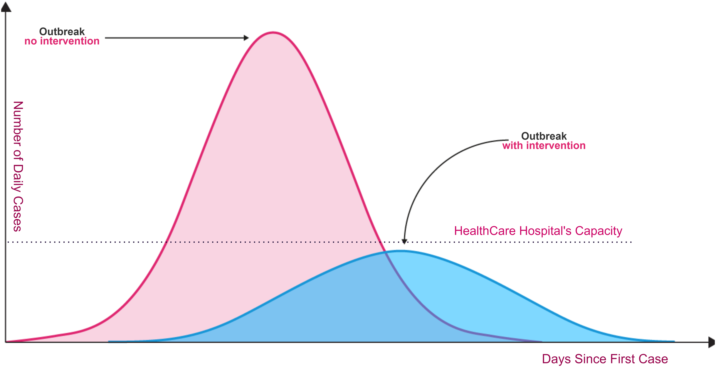
Unfortunately, the spread of COVID-19 is exponentially, and the transmission process is not clearly understood. Today, dealing with Coronavirus is an important healthcare challenge for humanity all over the world. Even though the Coronavirus infection in common incorporates small or no side effects, it causes lethal pneumonia in 2:8% of the infected patients (Hoehl et al., 2020; Lu et al., 2020; Sohrabi et al., 2020). Normally it takes 5:6 days from the disease day with the infection for indications to appear. However, it may take up to 14 days in some cases. As shown in Fig. 1, without rapid testing, the number of COVID-19 cases could increase beyond the healthcare system’s capacity to deal with serious cases (red curve in relation to healthcare system capacity line). Fast and accurate detection reduces the daily rate of new cases (flattening the blue curve).
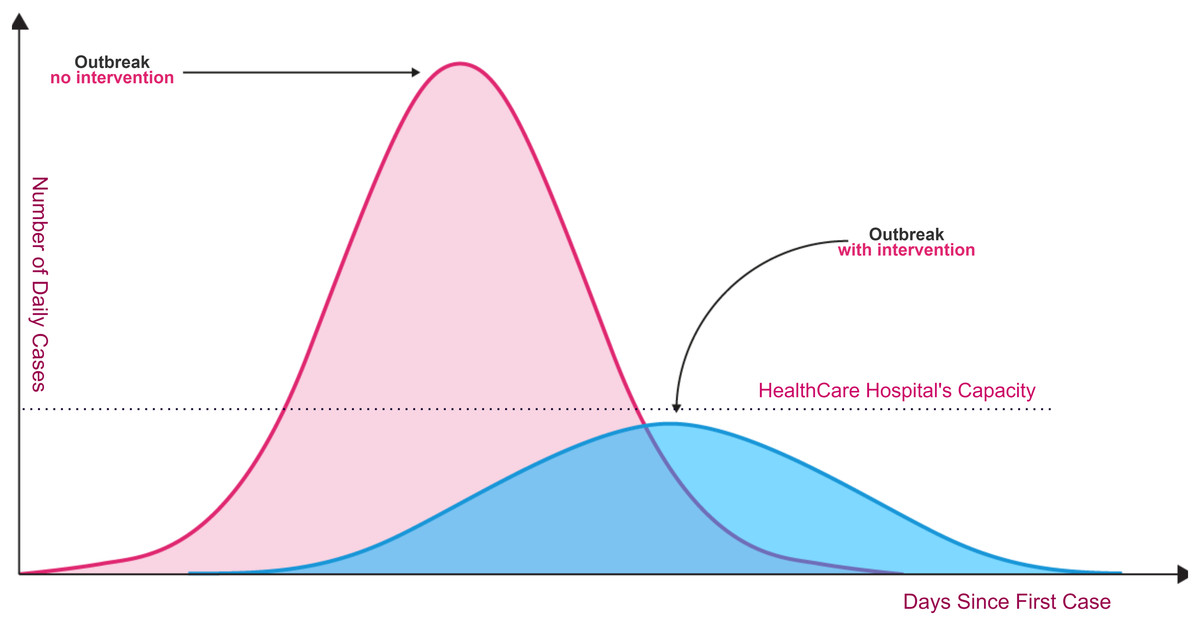
Figure 1: Coronavirus outbreaks and lowering infection rates (World Health Organization, 2020b).
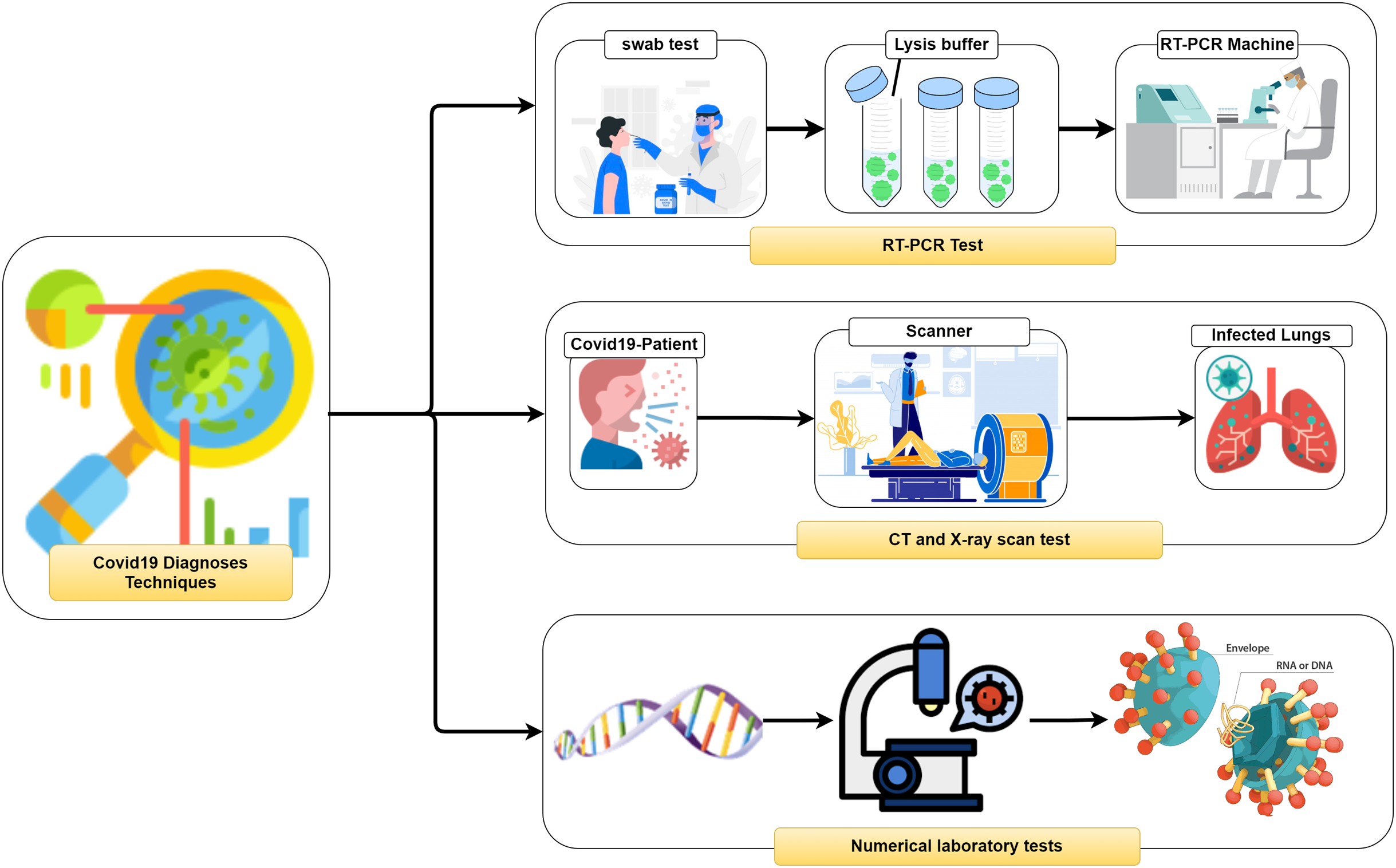
It is vital to distinguish (i.e., diagnose) the COVID-19 as quickly as conceivable and in an exact way to diminish the fast spread of the infection. In general, three different methodologies, as seen in Fig. 2, can be used to recognize COVID-19 patients as follows: (1) RealTime reverse transcriptase-polymerase Chain Reaction (RT-PCR), (2) Chest Computed Tomography (CT) imaging scan, and (3) Numerical laboratory tests. The current common strategy to recognize COVID-19 patients is the RT-PCR test (Ai et al., 2020) which is fairly sensitive and reliable. Unfortunately, depending only on the RT-PCR causes a remarkable delay in the diagnosis of the suspected patients. Besides, utilizing the RT-PCR test has numerous troubles within the extremely hit regions, particularly amid early flare-ups of this disease. On the other hand, the high false-negative rates are a true challenge for the test labs. Many factors affect the sample result, such as test planning and quality control (Liang, 2020).
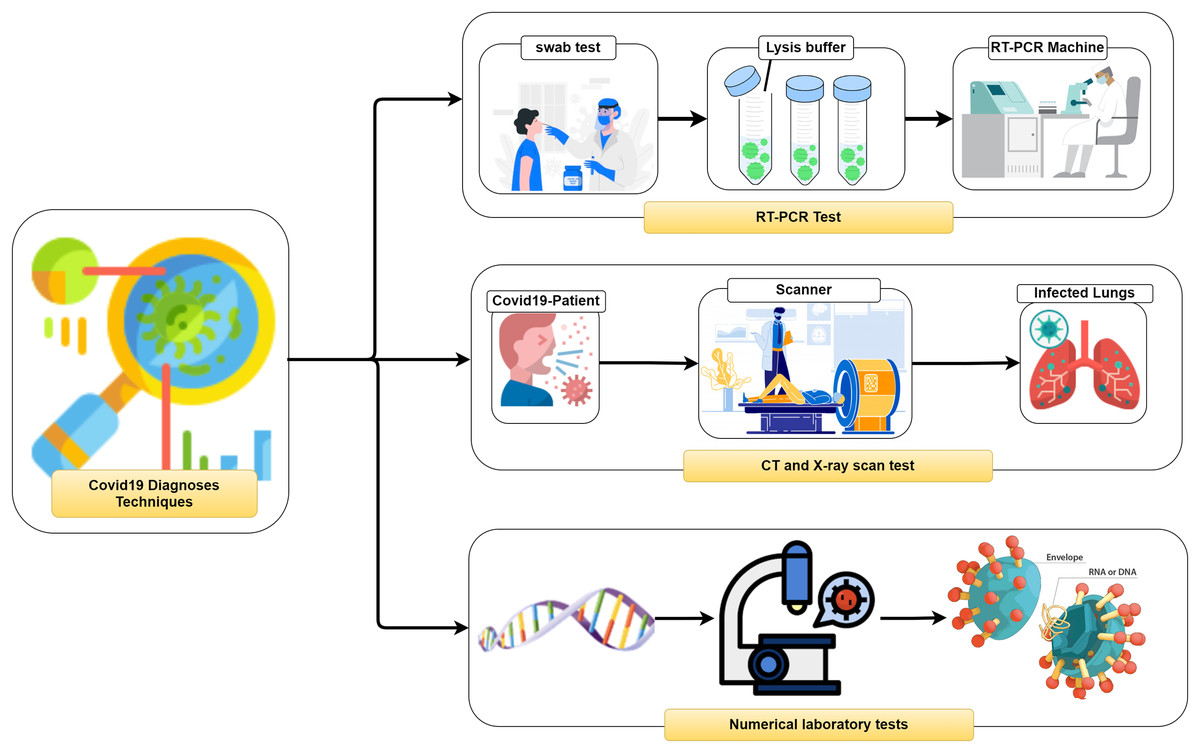
Figure 2: Coronavirus diagnose techniques.
As a result, chest imaging, such as chest CT or chest X-ray (CXR), is utilized as a first-line examination to detect the virus infection (Rubin et al., 2020; Wong et al., 2020). Chest imaging technologies, especially CXR, are broadly accessible and economical. For this reason, radiologists use chest imaging to detect early lesions in the lung at high speed and sensitivity. Concerning the COVID-19, several aspects of lung anomaly such as bilateral abnormalities, interstitial abnormalities, lung consolidation, and ground-glass opacities are showed in chest images (Guan et al., 2020). Consequently, examining the suspected patients’ chest images presents an essential part remarkable potential for screening processes, and early determination of COVID-19 disease (Kandaswamy et al., 2014). Unfortunately, the diagnosis process mainly relies on the radiologists’ visual diagnosis, which leads to many issues. At first, it takes an exceptionally long time to diagnose since chest imaging contains hundreds of slices, which takes a long time to analyze. Much other pneumonia has similar aspects to COVID-19, so, only radiologists with accumulative experience to diagnose COVID-19 disease.
The artificial intelligence (AI) branch, especially deep learning (DL), has been used to automatically identify lung diseases in medical imaging with significantly diagnostic accuracy (Guan et al., 2020; Rubin et al., 2020). Deep learning is efficient in dealing with the medical dataset, particularly those datasets containing a huge number of training samples. Recently, many research papers address the detection of COVID-19 pneumonia and classify the severity of COVID-19. These research studies try to automatically detect the infected patients early to help society by isolating them to prevent or decrease the native spread. Deep transfer learning (DTL) is a deep learning approach trained on a source problem and then reused to solve a target problem. DTL can be used for two reasons: (1) the transfer of the extracted features from the source issue (Kandaswamy et al., 2014) and (2) the retrain of only the network unfrozen layers by constraining not to over train for the target mission (Yosinski et al., 2014). Employing Convolution Neural networks (CNN) using Transfer Learning is recently used to achieve very promising approaches to diagnose several diseases such as cancer (Bhatt, Ganatra & Kotecha, 2021) and Parkinson (Suzuki, 2017).
Although the research applied in convolutional neural network architectures achieved promising results to detect the COVID-19, the huge number of existing hyperparameters still represents a challenge to achieve better and promising results (Ng et al., 2020). There are recent investigations to optimize CNN’s hyperparameters by utilizing metaheuristics. The hyperparameters of the CNN network, such as learning rate, kernel size, and kernel type of convolutional blocks, should be tuned to enhance the network’s performance.
Zhao, Zhang & Wang (2020) proposed the Manta Ray Foraging Optimization (MRFO) algorithm, inspired by manta rays’ intelligent behaviors. MRFO overcomes the major drawbacks of well-known metaheuristics algorithms, such as slow search speed and easy premature convergence. MRFO outperforms the other optimization algorithms to search precision, convergence rate, stability, and local optimal value avoidance (Wong et al., 2020). This study suggests using the MRFO algorithm to fine-tune the CNN network’s hyperparameters to achieve more accurate results.
This study’s main objective is to introduce an Optimized Transfer Learning-based Approach for Automatic Detection of COVID-19 (OTLD-COVID-19). The OTLD-COVID-19 approach performs the classification and recognition of the lung X-ray images for COVID-19 diseases. The OTLD-COVID-19 approach uses CNN and MRFO algorithm for the parameters and hyperparameters optimizations, respectively. The rest of the paper is structured as follows: “Background” represents the CNNs and MRFO Algorithm theoretical background. “Related Work” discusses the related work. “The Proposed OTLD-COVID-19 Approach” shows the proposed OTLD-COVID-19 approach details. The results, achieved by the proposed technique, are presented in “Experiments, Results and Discussion”. Finally, the conclusions and future work are drawn.
Paper contributions
In this paper, an approach for automatically detecting COVID-19 using transfer learning is proposed to achieve diagnosis reliably. The OTLD-COVID19 approach works on lung X-ray images to achieve both recognition and classification of COVID-19 diseases. This approach aims to achieve high performance in both processes. To that end, it seeks the best hyperparameters combination to optimize CNN’s parameters. There are many meta-heuristics optimization algorithms with different approaches, including try-and-error, deterministic, and stochastic. This study uses a meta-heuristic optimizer to search the scope automatically. In this vein, to improve the classification performance, the OTLD-COVID-19 approach utilized CNN and MRFO algorithm for the automatic parameters and hyperparameters optimization respectively. The OTLD-COVID-19 approach is used as a pillar to improve overall accuracy and reduce computational cost. The contributions of the current study are summarized in points as follow:
-
Proposing the OTLD-COVID-19 approach for rapid COVID-19 diagnosis using automated X-ray image processing.
-
Twelve popular CNN architectures, with four classes (“COVID-19,” “Bacterial Pneumonia,” “Viral Pneumonia,” and “Normal”), are used in the transfer learning technique for the detection of COVID-19 patients.
-
The Manta-Ray Foraging Optimization (MRFO) algorithm is used to optimize the network hyperparameters’ values to enhance the classification performance.
-
The proposed technique is adaptable and scalable; there is no need to manually assign the CNN architecture’s hyperparameters values.
-
Regularization, optimization, dropout, and data augmentation are studied through the different reported experiments.
-
The proposed technique is compared with the other state-of-the-art techniques and studies. The achieved results of the standard performance metrics are very promising.
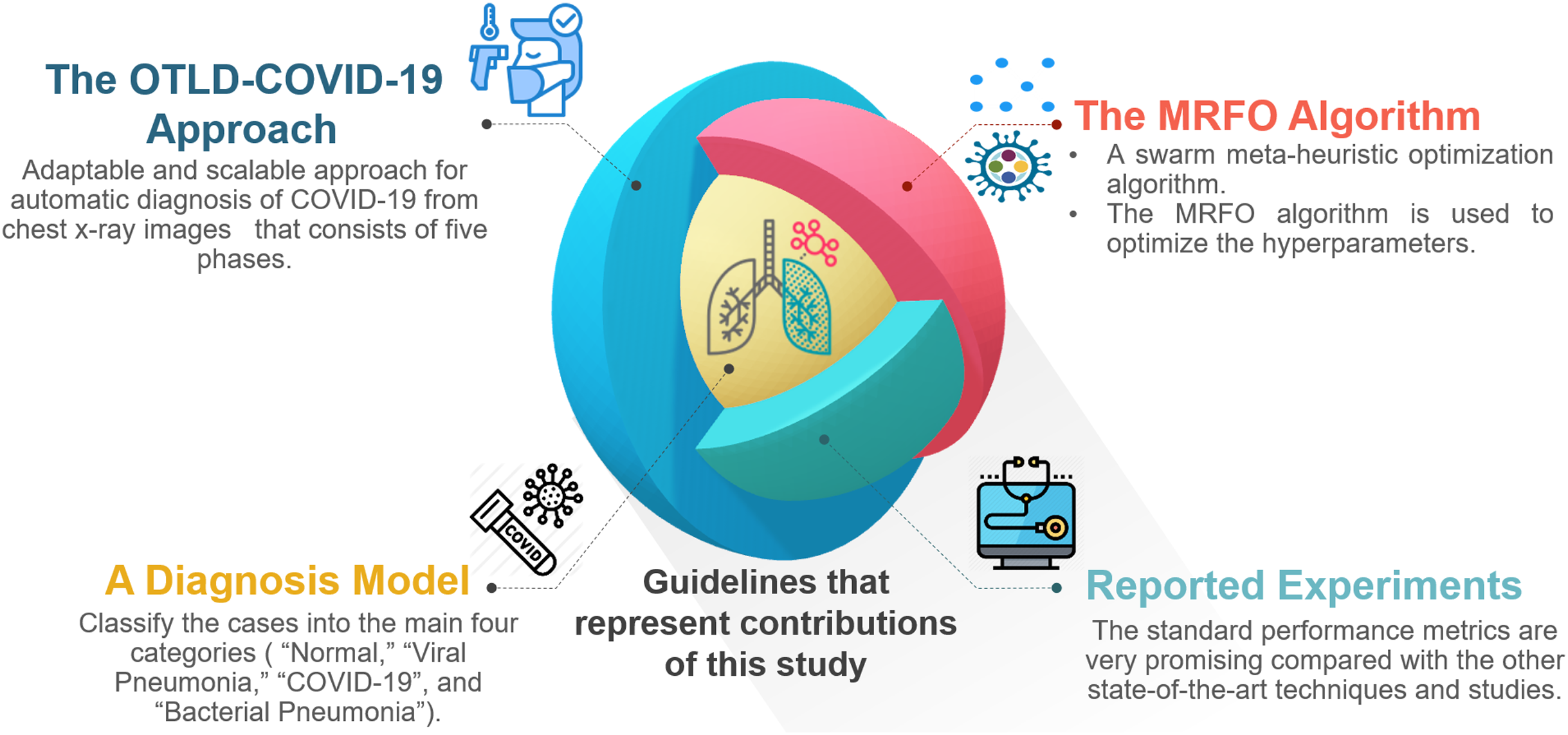
For the convenience of readers, Fig. 3 depicts the guidelines of the four primary sections that reflect the contributions of this study. First, “The Proposed OTLD-COVID-19 Approach” introduces the proposed OTLD-COVID-19 approach. The OTLD-COVID-19 approach is characterized by its adaptability and scalability. It consists of five phases: (1) Acquisition phase, (2) Preprocessing phase, (3) Augmentation phase, (4) Training, Classification, and Optimization (TCO) phase, and (5) Deployment phase. Second, “The Proposed OTLD-COVID-19 Approach” illustrates the MRFO algorithm, which uses various foraging mathematical models to optimize the key hyperparameters’ values automatically. Third, the deployment phase of the proposed approach uses computed hyperparameters to build a diagnostic model. Each model evaluates the COVID-19 dataset to classify the cases into the main four categories (i.e., “COVID-19,” “Bacterial Pneumonia,” “Viral Pneumonia,” and “Normal”). Fourth, in “Experiments, Results and Discussion”, different reported experiments are introduced. The achieved results of the standard performance metrics are very promising compared with the other state-of-the-art techniques and studies.
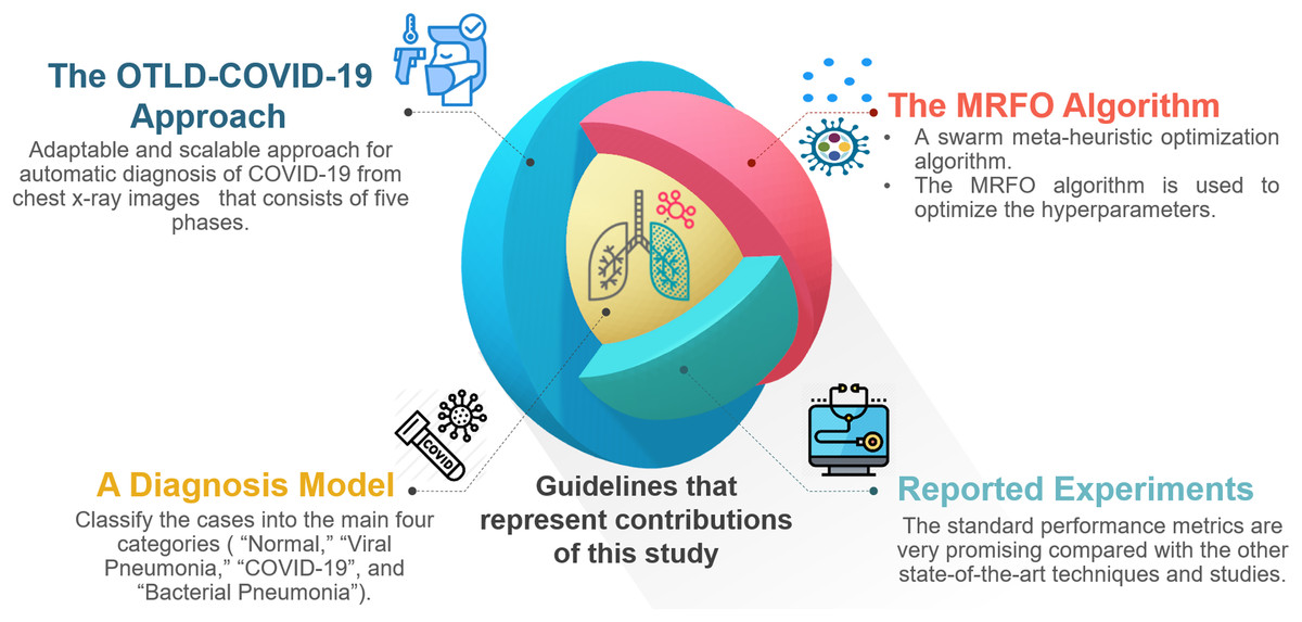
Figure 3: The guidelines that represent the contributions of this study.
In a summary, our OTLD approach improves the network performance in several ways. First, due to the lack of COVID 19 data, the proposed dataset is created from eight different datasets to increase the amount of data and avoid overfitting. Second, the MRFO optimization algorithm is used to obtain the optimal values of network hyperparameters. MRFO overcomes the main drawbacks of well-known metaheuristic algorithms, such as slow search speed and slight premature convergence. MRFO outperforms the other optimization algorithms in terms of search precision, convergence rate, stability, and local optimal value avoidance. Third, Transfer Learning (TL) is used to achieve the best network performance. Here, the MRFO optimization algorithm is applied to twelve different CNN architectures to obtain the best combination of hyperparameters for each architecture and obtain the architecture with the best performance. Finally, many performance metrics are measured to ensure the competence of the architecture with the best performance.
Background
CNN architectures
There is a continuous research investigation in the CNN architectures, and, notably, the noteworthy achievement in the CNN performance happened from 2015 to 2019. Khan et al. (2019) classified the CNN architectures into seven main categories. In this section, the most applicable CNN architectures from the mentioned classes are described. AlexNet (Antonellis et al., 2015) is designed to be the first known deep CNN architecture. AlexNet increases CNN’s depth by applying many different parameter optimization strategies to improve the learning capacity of the CNN (Antonellis et al., 2015). Although increasing the depth enhanced the generalization for different image resolutions, it caused the network to suffer from overfitting problems. Krizhevsky, Sutskever & Hinton (2012) adopted the idea of Hinton (Dahl, Sainath & Hinton, 2013; Srivastava et al., 2014) to solve the overfitting problem. They enforced the model to learn more robust features through skipping some transformational units randomly during the training process. Moreover, they used the Rectified Linear Unit (ReLU) activation function to enhance the convergence rate by mitigating the vanishing gradient issue (Nair & Hinton, 2010).
Simonyan & Zisserman (2014) proposed VGG, a CNN architecture designed simply and efficiently. It has 19 layers deeper than AlexNet to simulate the relationship between the network depth and capacity (Antonellis et al., 2015; Hodan, 1954). VGG addressed the large-size filter effect by replacing the large-size filter with a stack of (3 × 3) filters. Using the small-size filters enhanced the computation complexity. Unfortunately, the VGG still had a huge number of parameters, leading to severe difficulties in deploying it on low resource systems. Wu, Zhong & Liu (2018) proposed the CNN’s residual learning principle and efficiently trained the deep networks. ResNet presented a deeper network with less computational complexity than the previously proposed networks. ResNet is deeper than AlexNet and VGG by 20 and eight times, respectively (Simonyan & Zisserman, 2014).
The GoogleNet architecture was designed mainly to enhance the accuracy by reducing the computational cost (Szegedy et al., 2015). For this reason, the CNN inception block principle is presented where the conventional layers are replaced in small blocks (Lin, Chen & Yan, 2013). Each block has different size filters to get the spatial data at diverse scales. Inception-V3, Inception-V4, and Inception-ResNet are modified and enhanced versions of Inception-V1 and Inception-V2 (Roos & Schuttelaars, 2015; Szegedy et al., 2015; Szegedy et al., 2016). The main concept of Inception-V3 is to reduce the computational cost of deep networks without influencing the generalization. For that reason, Szegedy et al. (2016) used small and asymmetric filters ((1 × 5) and (1 × 7)) instead of large size filters ((5 × 5) and (7 × 7)). Besides, they used (1 × 1) convolution as a bottleneck in the front of the large filters. In Inception-ResNet, Szegedy et al. (2016) combined both the power of residual learning and inception block.
DenseNet was mainly designed to handle the vanishing gradient issue. ResNet specifically holds information through additive identity transformations; it suffers from a series problem, resulting in several layers that can contribute very little or no information (Blei, Ng & Jordan, 2003). DenseNet employed cross-layer connectivity differently. A feed-forward fashion is used to connect each previous layer to the next coming layer. The network’s information flow is substantially improved as DenseNet used the loss function to grant each layer direct access to the gradients. Xception is known to be an extreme Inception architecture, where the concept of a depth-wise separable convolution is embraced (Chollet, 2017) Xception achieved significant enhancements since it broadened the original inception block and regulated the computational complexity. The different spatial dimensions ((1 × 1), (5 × 5), and (3 × 3)) are replaced by a single dimension (3 × 3) followed by a (1 × 1) convolution. Also, Xception convolved each feature map in a separate way to get easier computations.
ResNet extended and improved the Inception Network (Xie et al., 2017). The authors applied the concept of splitting, transforming, and merging efficiently and simply. Besides, the cardinality concept is introduced (Szegedy et al., 2015). Cardinality is an extra dimension, which refers to the size of the set of transformations (Han et al., 2018; Sharma & Muttoo, 2018). The Inception network enhanced the convolution CNNs learning capability and ensured the efficient use of network resources. MobileNet (Howard et al., 2017) is a recent class of deep learning architectures explicitly designed for quick inference on mobile devices. MobileNets and other conventional models’ key difference is that two more efficient stages are added than the standard convolutional operation is decomposed into two more efficient stages. The depthwise separable convolutions are used to perform a single convolution on each color channel rather than combining all three and flattening it. In MobileNet V1, the pointwise convolution either kept the number of channels the same or doubled them. At the same time, MobileNetV2 (Sandler et al., 2018) decreases the number of channels. Table 1 compares the various CNN architectures.
| Architecture | Parameters | Error rate | Category |
|---|---|---|---|
| AlexNet | 60 M | ImageNet: 16.4 | Spatial Exploitation |
| VGG | 138 M | ImageNet: 7.3 | Spatial Exploitation |
| GoogLeNet | 4 M | ImageNet: 6.7 | Spatial Exploitation |
| ImageNet: 3.5 | |||
| Inception-V3 | 23.6 M | Multi-Crop: 3.58 | Depth + Width |
| Single-Crop: 5.6 | |||
| Inception-V4 | 35 M | ImageNet: 4.01 | Depth +Width |
| Inception-ResNet | 55.8 M | ImageNet: 3.52 | Depth + Width + Multi-Path |
| ResNet | 25.6 M | ImageNet: 3.6 | Depth + Multi-Path |
| 1.7 M | CIFAR-10: 6.43 | ||
| Xception | 22.8 M | ImageNet: 0.055 | Width |
| CIFAR-10: 3.58 | |||
| CIFAR-100: 17.31 | |||
| ResNeXt | 68.1 M | ImageNet: 4.4 | Width |
| 25.6 M | CIFAR-10+: 3.46 | ||
| DenseNet | 25.6 M | CIFAR100+: 17.18 | Multi-Path |
| 15.3 M | CIFAR-10: 5.19 | ||
| 15.3 M | CIFAR-100: 19.64 | ||
| MobileNet-V1 | 4.2 M | ImageNet: 10.5 | Depth + Width |
| MobileNet-V2 | 3.5 M | ImageNet | Depth + Width |
Transfer learning and CNN hyperparameters
Transfer learning is an effective representation learning approach in which the learned knowledge gained from a certain mission is used to enhance generalization about another. Transfer learning is much recommended when the number of images from the available datasets is relatively small. In this case, the original architecture and its weights are preserved and can be reused, especially when the used dataset in training the original architecture is vast. For example, the network architectures trained on the ImageNet dataset such as VGG (Simonyan & Zisserman, 2014) and DenseNet (Blei, Ng & Jordan, 2003) are extremely useful in medical image processing since it keeps the features of medical images in the ImageNet dataset. There are two common strategies to apply transfer learning: feature extraction and fine-tuning. In the feature extraction strategy, the last feed-forward layer(s) of the network is frozen. So, not all the weights are optimized; only the newly added layers are optimized during training. In the fine-tuning strategy, the pre-trained network is used as a starting point, and none of the weights are frozen, so all the network weights are optimized for the new task (Alshazly et al., 2019; Azizpour et al., 2015). When a fine-tuning strategy is adopted, it is recommended to apply lower learning rates to the pre-trained network to avoid the initial weights’ destruction.
Hyperparameters tuning is essential since it controls the overall behavior of a learning model. The main objective of tuning the hyperparameters is to get an optimal combination of hyperparameters that minimizes a predefined loss function to improve the network performance. CNN hyperparameters are classified into two main categories. The hyperparameters related to the network structure and The hyperparameters that determine how the network is trained. The main hyperparameters of both categories are described in Table 2.
| Category | Hyperparameters | Definition |
|---|---|---|
| Network Structure | Hidden layers | It represents the number of layers between the input and output layer. |
| Kernel Size | It indicates the height and width of the 2D convolution window. | |
| Kernel Type | It specifies the applied filter (e.g. edge detection, sharpen). | |
| Stride | It specifies the step size of the kernel when crossing the image. | |
| Padding | The extra pixels of filler around the boundary of the input image that are set to zero. | |
| Dropout | It defines the percentage of neurons that should be ignored to prevent overfitting. | |
| Activation Functions | They are the mathematical equations that allow the model to learn nonlinear prediction boundaries. | |
| Training Methodology | Learning Rate | It defines how quickly a network updates its parameters. |
| Momentum | It specifies the value to let the previous update affect the current weight update. | |
| The Epochs Number | The number of iteration when the dataset is trained. | |
| Batch Size | It defines the number of patterns applied to the network before the weights are updated. | |
| Optimizer | It defines the parameters updating technique. |
Several methods are used to determine the hyperparameters’ values, including manual search, grid search, random search, and optimization techniques. This paper proposes using the MRFO optimization technique to find out the values of the hyperparameters.
Manta ray foraging optimization
Manta Ray Foraging Optimization (MRFO) (Zhao, Zhang & Wang, 2020) is a swarm meta-heuristic optimization algorithm bio-inspired by a foraging strategy practiced by the manta rays to capture the prey. Manta rays have developed various powerful and intelligent foraging strategies, such as chain foraging, cyclone foraging, and somersault foraging. Chain foraging mimics the intrinsic behavior of the food search. Foraging manta rays line up in an organized fashion to capture lost preys missed or unnoticed by the chain’s previous manta rays. This cooperative interaction between rival manta rays decreases the risk of prey loss while also increasing food rewards. Cyclone foraging occurs when there is a high density of prey. The tail end of the manta ray connects with its head forming a spiral to produce a vertex in the eye of a cyclone, causing the filtered water to rise to the surface. This complex mechanism allows a manta ray to capture the prey easily. The last foraging strategy is the somersault foraging. When manta rays find a food source (plankton), they perform backward somersaults before circling around the plankton, pulling it towards them. These foraging behaviors are extremely successful, despite their rarity in nature. The following sections cover the mathematical models for each foraging strategy. It worth mentioning that the used symbols in the current study for the MRFO models are similar to the MRFO original paper to avoid misunderstandings.
Chain foraging
Manta rays hunt for prey plankton and swim towards it after determining its location. The best location is one with a higher plankton concentration. Manta rays form a foraging chain by forming a line from head to tail. Each manta ray adjusts its position based on the best solution achieved so far and the location of the one in the front. Figure 4 shows the chain behavior.

Figure 4: Chain foraging behavior in the 2-D space illustration (Zhao, Zhang & Wang, 2020).
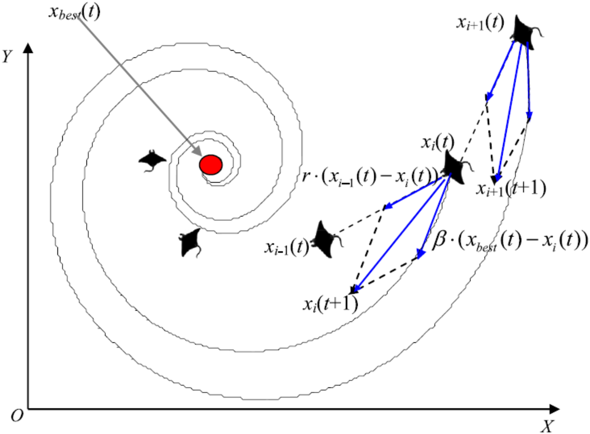
Cyclone foraging
When a group of manta rays recognizes a plankton group in deep water, they form a foraging chain and make spiral movements as they approach the food source. During the cyclone foraging process, flocked manta rays not only pursue the manta ray in front of them to ensure the chain’s continuity, but they also chase a spiral pathway to get to the target prey. Figure 5 shows the cyclone behavior.
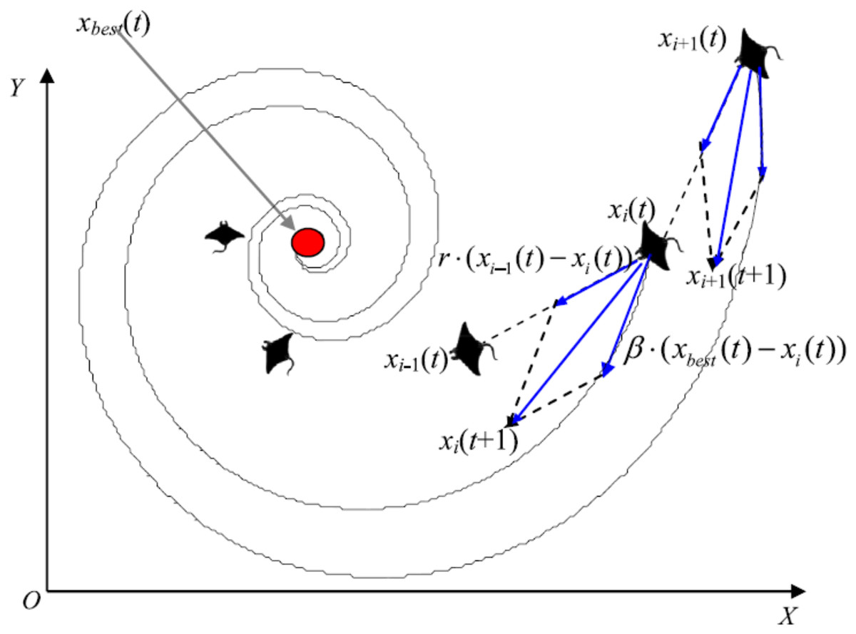
Figure 5: Cyclone foraging behavior in the 2-D space illustration (Zhao, Zhang & Wang, 2020).
Somersault foraging
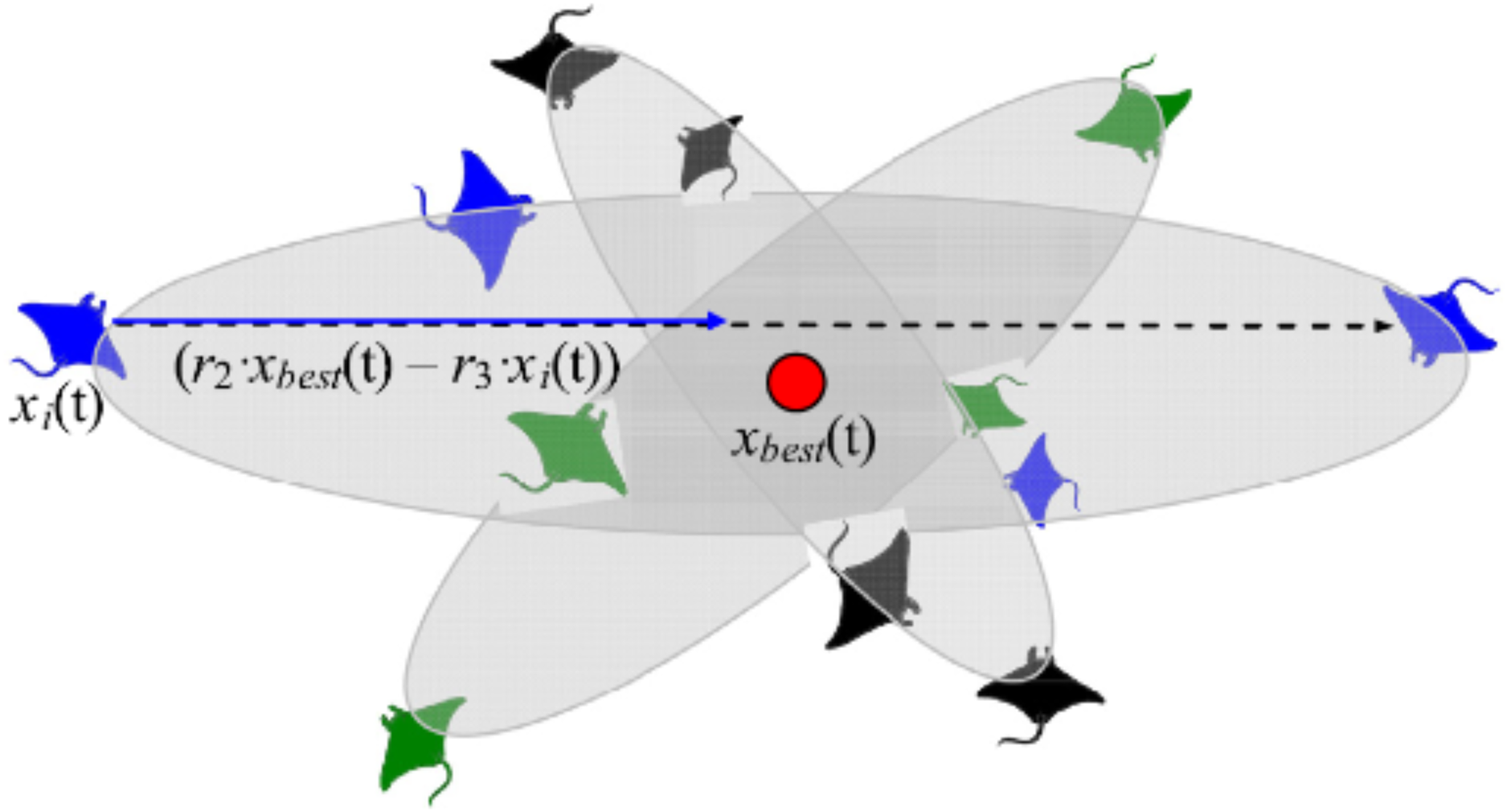
This foraging scheme considers the best prey location as a pivot point. Each manta-ray in the population searches around this point to migrate to a new location in the search domain. In the search space, all individuals progressively approximate to the optimal solution. As a result, the range of somersault foraging is reduced as iterations increase. Figure 6 demonstrates the pattern of somersault foraging in MRFO.
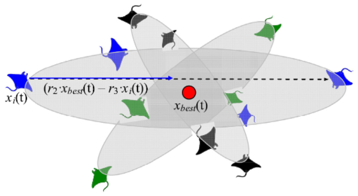
Figure 6: Somersault foraging behavior in the MRFO illustration (Zhao, Zhang & Wang, 2020).
Related work
Convolutional Neural Network (CNN) is considered one of the most effective deep learning approaches for accurately analyzing medical images. The main features to identify the COVID-19 in medical images include bilateral distribution of patchy shadows and ground-glass opacity (Wang et al., 2020). The research effort in the COVID-19 detection can be classified into three different perspectives related to deep learning techniques. These perspectives are tailored to CNN, transfer learning, and hybrid architectures. This section discusses the research studies to automate the detection of the COVID-19 according to these perspectives.
A tailored CNN Architectures is a CNN network designed specifically to detect the COVID-19. The network is trained for the time. Mukherjee et al. (2020) introduced introduced a shallow CNN architecture consisting of four layers. Light architecture is to minimize the number of parameters (i.e., weights) to speed up computational time. Besides, the shallow (or lightweight) CNN design avoids possible overfitting that faces architectures with heavy usage of parameters. The shallow CNN architecture is well fit for mass population screening, especially in resource-constrained areas. The tailored shallow CNN model is designed to diagnose 2 class classification (“COVID” and “Normal”). It achieved an accuracy, sensitivity, and (Area Under Curve) AUC of 96.92%, 0.942, and 0.9869 respectively.
Wang, Lin & Wong (2020) introduced COVID-Net, a tailored deep CNN architecture for detecting the COVID-19 cases using CXR images. They claimed that COVID-Net is one of the first open-source network designs for COVID-19 detection. They also introduced COVIDx, an open-access benchmark dataset with 13,975 CXR images representing 13,870 patient cases. The COVIDx dataset is generated by combining and modifying five open access existing datasets having chest scans. Their experimental results showed the achieved accuracy is 92.4% to classify “Normal,” “non-COVID Pneumonia,” and “COVID-19” classes.
Majeed et al. (2020) introduced CNN-X, a tailored CNN architecture that holds four parallel layers. Each layer has 16 filters in three different sizes (3 × 3), (5 × 5), and (9 × 9). (3 × 3) filters detect the local-features while global features are detected by (9 × 9) filter. The (5 × 5) filter is used to detect what is missed by the other two filters. Then, the convolved image is applied to batch normalization and a ReLU activation function. Afterward, average pooling and maximum pooling are applied. The reason for using different size filters is to detect. They used Two COVID-19 X-ray image datasets in addition to a large dataset for other infections.
Hammoudi et al. (2020) proposed a tailored CNN architecture to handle the two data modalities (CT and X-rays). Their model consists of nine layers for detecting COVID-19 positive cases. They trained and tested their network using both CT scans and X-rays. The experimental results show that their architecture achieved an overall accuracy of 96.28%.
Hussain et al. (2021) presented a CoroDet, a tailored 22-layer CNN architecture to detect COVID-19 using both chest X-ray and CT modalities. The architecture consists of several layers: convolution layer, pooling layer, dense layer, flatten layer, and three activation functions. The CoroDet is designed to diagnose 2 class classification (“COVID-19” and “Normal”), 3 class classification (“COVID-19”, “Normal”, and “Pneumonia”), and 4 class classification (“COVID-19”, “Normal”, “non-COVID Viral Pneumonia”, and “non-COVID Bacterial Pneumonia”). Their architecture’s accuracy varies from 99.1% for the two classes to 91.2% for the four classes classification.
Traditional transfer learning strategies are promising since the COVID-19 pneumonia CXR data is very limited. In this work, the popular deep learning architectures are customized to the purpose of the COVID-19 detection. Only the last few layers of the pre-trained model are replaced and retrained. The modified CNN architecture gets the advantages from the base CNN. The learned feature representations are fine-tuned to improve performance. Farooq & Hafeez (2020) suggested using the ResNet50 architected. They replaced the head of the trained model with another head containing a sequence of Adaptive average/max pooling, batch normalization, drop out, and linear. The ResNet50 weights are pre-trained using the ImageNet dataset that has X-ray images with different sizes.
Apostolopoulos & Mpesiana (2020) tested five standard CNN architectures, including VGG19, InceptionNet, MobileNetV2, XceptionNet, and Inception. Different hyperparameters are used to identify the COVID-19. They used two different datasets having X-ray images from public medical repositories. Their results showed that the best-achieved accuracy, sensitivity, and specificity are 96.78%, 98.66%, and 96.46%, respectively, obtained from MobileNetV2 architecture. Narin, Kaya & Pamuk (2020) used five pre-trained convolutional neural network-based models to identify the COVID-19 using chest X-ray images. They implemented three different binary classifications with four classes (“COVID-19”, “Normal” (i.e., “Healthy”), “Viral Pneumonia,” and “Bacterial Pneumonia”). The results showed that the pre-trained ResNet50 model achieves the best classification performance.
Islam et al. (2020) performed modality-specific transfer learning through retraining the ImageNet Network on the RSNA CXR collection to learn CXR modality-specific features and detect the abnormality. The used collection contains both normal CXRs and abnormal images having pneumonia-related opacities. Dropout is used to overcome overfitting where the regularization is restricted, and generalization is improved by reducing the model sensitivity to the training input’s specifics. The different hyperparameters of the CNNs are optimized using a randomized grid search method.
Nayak et al. (2021) introduced a deep Learning architecture to automate the COVID-19 detection using X-ray images. They evaluated the performance of eight CBB architectures to detect COVID-19 cases. The introduced architectures are compared by considering several different hyperparameters values. The results showed that the ResNet-34 model achieved a higher accuracy of 98.33%. Khan, Shah & Bhat (2020) presented CoroNet architecture, a pre-trained CNN architecture to detect COVID-19 pneumonia from three different kinds of pneumonia using CXR images. The CNN architecture relies on Exception (Extreme Inception) and contains 71 layers trained on the ImageNet dataset. The authors introduced a balanced dataset containing 310 normal, 330 bacterial, 327 virals, and 284 COVID-19 resized CXR images. The experimental results showed that the CoroNet architecture achieved an accuracy of 0.87 and an F1-score of 0.93 for the COVID-19 detection.
In most typical deep learning architectures, the CNN is used for both feature extraction and classification. Combined architectures use CNN either for feature extraction and apply another classifier to identify the COVID-19 patients or classify and use other algorithms to extract and optimize features. The hybrid architecture combines different deep learning algorithms or combines deep learning with other AI models such as machine learning and data mining.
Islam, Islam & Asraf (2020) introduced a deep learning architecture that combines a CNN and a Long Short-term Memory (LSTM) to identify the COVID-19 from X-ray images automatically. They used the CNN network to extract deep features and LSTM for the detection of the COVID-19 patients. Another study (Islam et al., 2020) introduced architecture to diagnose the COVID-19 using chest X-rays. The architecture combined CNN for feature extraction and recurrent neural network (RNN) for classification to diagnose the COVID-19 from chest X-rays. They used many deep transfer techniques, including VGG19, DenseNet121, InceptionV3, and InceptionResNetV2. They showed that the performance of VGG19-RNN is better than the other compared architectures in terms of accuracy and computational time in our experiments.
Aslan et al. (2021) presented a hybrid architecture that combines the CNN and Bi-directional Long Short-term Memories (BiLSTM). They utilized the modified AlexNet (mAlexNet) architecture with chest X-ray images to diagnose the COVID-19. They modified the last three layers of the AlexNet model to build a three-class model classify the COVID-19. The remaining parameters of the original AlexNet model have been preserved. The temporal features obtained from the BiLSTM layer are passed as input to a fully-connected (FC) layer, and the Softmax is used for the classification.
Sethy et al. (2020) proposed a hybrid architecture that relies on ImageNet pre-trained models to extract the high-level features and Support Vector Machine (SVM) to detect the COVID-19 cases. Their architecture is a three-class problem to classify the COVID-19 patient from healthy people and pneumonia patients using X-ray images. They showed that the SVM achieved the best results when the features are extracted using the ResNet50 Network.
Altan & Karasu (2020) presented a combined architecture to detect the COVID-19 patients from X-ray images. The architecture consists of three different techniques: two-dimensional (2D) curvelet transformation, Chaotic Salp Swarm Algorithm (CSSA) optimization algorithm, and deep learning technique. 2D Curvelet transform is used to get the feature matrix from the patient’s chest X-ray images. An optimization process is done to the feature matrix. The EfficientNetB0 model, based on CNN, is used to classify X-ray images to diagnose the infected COVID-19.
The proposed otld-covid-19 approach
Recently, the COVID-19 pandemic has taken the world’s health care systems by surprise. It will also take a long time to ensure the vaccine’s safety before the general public could use it. As a result, the government’s existing efforts primarily focus on preventing the spread of COVID-19 and forecasting potential pandemic areas. Due to the scarcity of COVID-19 testing kits, particularly in developing countries, alternative diagnosis methods are essential. One solution is to develop COVID-19 diagnosis strategies based on data mining and artificial intelligence.
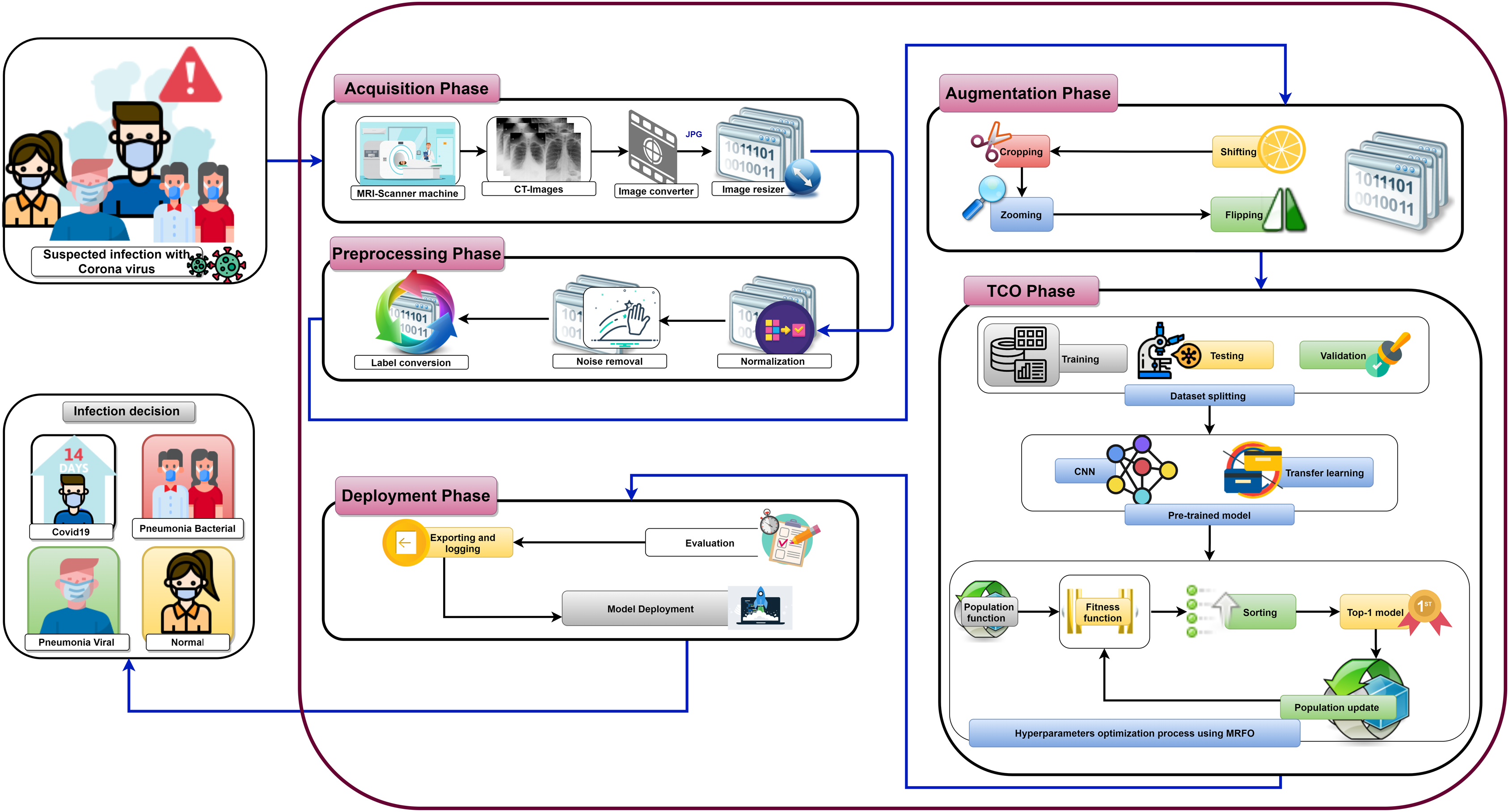
Figure 7 shows the proposed OTLD-COVID-19 approach that consists of five phases: (1) Acquisition phase, (2) Preprocessing phase, (3) Augmentation phase, (4) Training, Classification, and Optimization (TCO) phase, and (5) Deployment phase. The acquisition phase starts with reading the dataset, converting images to the “JPG” format, and resize the images to (64, 64, 3). Normalizing the images X (i.e., ) is performed in the preprocessing phase, followed by noise removal and converting the labels (i.e., classes) from numeric to one-hot encoding. In one-hot encoding, each category is converted into a new column and assigned a 1 or 0 as notation for true/false (e.g. 2 will be [0, 1, 0, 0] for 4 classes).

Figure 7: The proposed OTLD-COVID-19 approach.
The first stage of data augmentation aims to equalize the number of images in each category via shifting, cropping, zooming, and flipping (horizontally, vertically, or both). The TCO phase is the main core of the proposed approach. The first stage splits the augmented dataset into three parts (training, testing, and validation). It applies the transfer learning to obtain a pre-trained CNN model with ImageNet. In this study, twelve different models are tested to create the pre-trained CNN model (i.e., DenseNet121, DenseNet169, DenseNet201, Xception, MobileNet, MobileNetV2, MobileNetV3Small, MobileNetV3Large, EfficientNetB0, ResNet50V2, ResNet101V2, and ResNet152V2). The second data augmentation stage is applied during the training. The training optimizes the learning parameters. The last stage in this phase is the hyperparameters optimization process.
The MRFO algorithm is repeated for several iterations (i.e., 15 in the current study) to optimize the main hyperparameters. It defines the population size (Np), maximum number of iterations (Ns) and dataset split ratio (SR). Random positions of the manta-rays are initialized before applying either chain or cyclone foraging according to a random value. MRFO starts the chain foraging if the random value is lower than 0.5. The chain foraging mathematical model is represented in Eqs. (1) and (2) as follows:
(1)
(2) where is the position of ith individual at time t in dth dimension, r is a random vector within the range of [0, 1], α is a weight coefficient, and is the plankton with the highest concentration.
The cyclone foraging process plays an important part in developing two key driving mechanisms: exploitation and exploration. The exploitation (intensification) aims to find the best candidate solutions in the current search space, called the local search. The exploration (the global search) is concerned with exploring different search space areas to avoid getting stuck in a local minimum. In this foraging process, the best plankton location is used as a reference point, allowing for increased exploitation capabilities by enlarging the fertile regions surrounding the current best solution. Eqs. (3) and (4) mathematically models the exploitation phase.
(3)
(4) where β is the weight coefficient, T is the maximum number of iterations, and r1 is a random number in the range [0, 1].
Cyclone foraging helps the exploration process by forcing the population members to shift to a random location in the search space. This position is far from their current location as well as the best prey location. This exploration method helps the algorithm extend the global search space and direct the population through the search domain’s unvisited paths. The mathematical model of the exploration process is given by Eqs. (5) and (6) below.
(5)
(6) where is a random position randomly produced in the search space, and LBd and UBd are the lower and upper limits of the dth dimension, respectively.
MRFO shifts between exploration phases according to the ratio between current iteration and the maximum number of iterations (ns/Ns). The exploitation phase is enacted when ns/Ns<rand. The technique switches to the exploration phase if ns/Ns>rand.
After completing either cyclone or chain foraging, summersault foraging takes action. It updates the current position of individuals through the current best solution. The following mathematical formulation (i.e., Eq. (7)) describes the summersault foraging.
(7) where S is the somersault factor that decides the somersault range of manta rays and its value equals 2, r2 and r3 are two random numbers in the range [0, 1].
The TCO phase computes the fitness score of each manta-ray and chooses the best individual. The metrics are determined from the evaluation of the trained model on the test part of the dataset. These metrics are used to calculate the overall fitness score after applying the trained model for several epochs (i.e., 64 in the current study). The calculated fitness score is used to update the position of manta-rays. This process repeats until the completion of the iterations (i.e. ns = Ns). Each result is evaluated, and a model is built according to the optimized computed hyperparameters. The model with these optimized hyperparameters is ready to achieve a rigid classification process. The pseudocode of the TCO is represented in Algorithm 1 where the “UpdateMRFO” function that uses the MRFO optimization algorithm is represented in Algorithm 2.
|
Input: Np, Ns, SR, Model // Population Size, Number of Iterations, Dataset Split Ratio, CNN Pre-trained Model Output: bestSoFar // The Best Combination Data: X, Y // Images Dataset, Images Labels POs ⇐ The Learning Parameters Optimizers BSs ⇐ The Learning Batch Sizes MLRs ⇐ The Learning Ratios DRs ⇐ The Learning Dropout Ratios Metrics ⇐ The Learning Performance Metrics ns ⇐ 1 // Initialize the Iterations Counter fitnessScores ⇐ [ ] trainX, validationX, testX, trainY, validationY, testY ⇐ DatasetSplit(X, Y, SR) // Get Np Solutions using a Random Initialization Process population ⇐ InitializePopulation(POs, BSs, MLRs, DRs, Np) // Find the Population Best Combinations using the Iterative Optimization Approach while ns ≤ Ns do // Find the Population Fitness Score Values of the Current Population np ⇐ 1 // Initialize the Populations Counter while np ≤ Np do solution ⇐ GetSolution(population, np) // Get the Solution at Index of np Model ⇐ LearnCNN(Model, solution, Metrics, trainX, trainY, validationX, validationY) // Apply the CNN Model Learning Proce (i.e. Train and Validate) metrics ⇐ TestCNN(Model, Metrics, testX, testY) // The the Optimized CNN using the Required Metrics fitnessScore ⇐ GetOverallFitnessScore(metrics) // Get the Overall Fitness Score using the Metrics’ Results fitnessScores.push(fitnessScore) // Append the Latest Fitness Score to the End of the List np ⇐ np + 1 // Increment the Populations Counter end sortedPopulation ⇐ SortFitnessScores(population, fitnessScores) // Sort the Population concrening the Fitness Score Values population ⇐ UpdateMRFO(sortedPopulation, POs, BSs, MLRs, DRs, Np) // Update the Population using the MRFO Algorithm ns ⇐ ns + 1 // Increment the Iterations Counter end bestSoFar ⇐ GetTop(population) // Extract the Overall Top Combination |
|
Input: population, bestFitness, Ns, ns, LB, UB, D // Population, The Best Fitness Score, Number of Iterations, Current Iteration, Lower Bound, Upper Bound, Number of Dimensions Output: newPopulation // The New Population newPopulation ⇐ Copy(population) Create a Copy from the Current Sorted Population bestSolution ⇐ newPopulation [1] Get the Best Solution (i.e., First Solution) From the Sorted Population coef ⇐ np ⇐ 1 Initialize the Populations Counter while (np ≤ Np) do r ⇐ random() // A Random Number in the Range [0, 1] r1 ⇐ random() // A Random Number in the Range [0, 1] α ⇐ 2.0 × r × // Calculate the Value of Alpha factor ⇐ β ⇐ 2.0 × exp(r1 × factor) × sin(2.0 × π × r1) // Calculate the Value of Beta if (random() < 0.5) then // Cyclone Foraging if (coef < random()) then rand ⇐ LB + random(D) × (UB − LB) if (np = 1) then newPopulation[np] ⇐ rand + r × (rand − newPopulation[np]) + β × (rand − newPopulation[np]) end else newPopulation[np] ⇐ rand + r × (newPopulation[np − 1] − newPopulation[np]) + β × (rand − newPopulation[np]) end end else if (np = 1) then newPopulation[np] ⇐ bestSolution + r × (bestSolution − newPopulation[np]) + β × (bestSolution − newPopulation[np]) end else newPopulation[np] ⇐ bestSolution + r × (newPopulation[np − 1] − newPopulation[np]) + β × (bestSolution − newPopulation[np]) end end end else // Chain Foraging if np = 1 then newPopulation[np] ⇐ newPopulation[np] + r × (bestSolution − newPopulation[np]) + α × (bestSolution − newPopulation[np]) end else newPopulation[np] ⇐ newPopulation[np] + r × (newPopulation[np − 1] − newPopulation[np]) + α × (bestSolution − newPopulation[np]) end end fitnessScore ⇐ GetFitnessScore(newPopulation[np]) // Get the Overall Fitness Score After Re-Learning the Model if (fitnessScore > bestFitness) then bestSolution ⇐ newPopulation[np] bestFitness ⇐ fitnessScore end Somersault Foraging S ⇐ 2.0 r2 ⇐ random() r3 ⇐ random() newPopulation[np] ⇐ newPopulation[np] + S × (r2 × bestSolution − r3 × newPopulation[np]) fitnessScore ⇐ GetFitnessScore(newPopulation[np]) // Get the Overall Fitness Score After Re-Learning the Model if (fitnessScore > bestFitness) then bestSolution ⇐ newPopulation[np] bestFitness ⇐ fitnessScore end end |
The deployment phase of the proposed approach uses computed hyperparameters to build a classification model. Each model evaluates the COVID-19 dataset to classify the cases into the main four categories (i.e., “Normal,” “Viral Pneumonia,” “COVID-19”, and “Bacterial Pneumonia”). The next section will discuss the experimental results of the proposed OTLD-COVID-19 approach compared to recent state-of-the-art approaches and explain its effectiveness.
Experiments, results and discussion
This section presents the different applied experiments with the corresponding results and discussions. It also presents the used dataset in the current study and ends by applying a comparative study between the current study and a set of state-of-the-art studies.
Dataset and experiments configurations
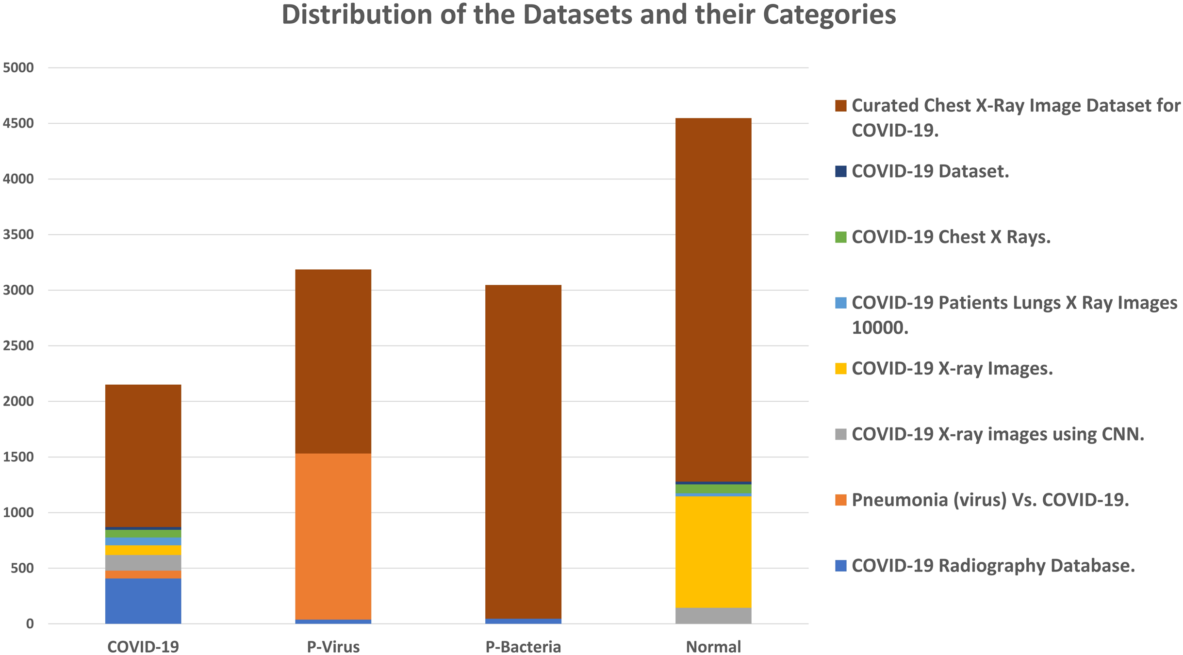
The adopted datasets in this study are real datasets used to distinguish COVID-19 from common pneumonia types. The proposed dataset is unified and collected from eight different public data sources described in Table 3 and graphically illustrated in Fig. 8. The dataset consists of chest X-ray images in four classes: radiographs of normal cases, viral pneumonia, COVID-19 pneumonia, and bacterial pneumonia. The total number of cases in the collected dataset is 12,933. Table 4 summarizes the common experiments configurations.

Figure 8: Distribution of the datasets and their categories.
| # | Dataset | COVID-19 | P-virus | P-bacteria | Normal |
|---|---|---|---|---|---|
| 1 | COVID-19 Radiography Database (Cohen et al., 2020). | 408 | 38 | 46 | 0 |
| 2 | Pneumonia (virus) Vs. COVID-19 (Mahasin, 2020). | 70 | 1,493 | 0 | 0 |
| 3 | COVID-19 X-ray images using CNN (Srikar, 2020). | 140 | 0 | 0 | 144 |
| 4 | COVID-19 X-ray Images (Das, 2020). | 88 | 0 | 0 | 1,002 |
| 5 | COVID-19 Patients Lungs X Ray Images 10000 (Sajid, 2020). | 70 | 0 | 0 | 28 |
| 6 | COVID-19 Chest X Rays (Sreeraman, 2020). | 69 | 0 | 0 | 79 |
| 7 | COVID-19 Dataset (Riaz, 2020). | 25 | 0 | 0 | 25 |
| 8 | Curated Chest X-Ray Image Dataset for COVID-19 (Sait, 2020). | 1,281 | 1,656 | 3,001 | 3,270 |
| Total | 2,151 | 3,187 | 3,047 | 4,548 | |
| Key | Value |
|---|---|
| Dataset | 8 Resources |
| Categories | “Normal”, “P-Viral”, “P-Bacterial”, and “COVID-19” |
| Dataset Size | 12,933 |
| Pre-trained Models | DenseNet121, DenseNet169, DenseNet201, Xception, MobileNet, MobileNetV2, MobileNetV3Small, MobileNetV3Large, EfficientNetB0, ResNet50V2, ResNet101V2, and ResNet152V2 |
| Parameters Initializer | ImageNet |
| Parameters Optimizers | Adam, NAdam, Ftrl, AdaDelta, AdaGrad, AdaMax, RMSProp, and SGD |
| Output Activation Function | SoftMax |
| Model Learn Ratios | [0 : 5 : 100]% |
| Batch Sizes | [8 : 8 : 100] |
| Dropout Ratios | [1 : 1 : 60]% |
| Number of Epochs | 8 Epochs |
| Performance Metrics | Accuracy, Loss, Precision, F1-score, AUC, Dice Coef., IoU Coef., Specificity, and Recall |
| Number of Iterations Ns | 20 Iterations |
| Population Size Np | 10 Candidates |
| Split Ratio SR | 85% to 15% |
| Image Size | (64, 64, 3) |
| Data Augmentation | Applied (in Two Stages) |
| Training Environment | Google Colab (using its GPU) |
Performance metrics
During the next experiments, there are different metrics to evaluate the performance of the “OTLD-COVID-19” approach. At first, the confusion matrix that represents a summary of predicted results is constructed. The confusion matrix has four values as follows:
-
True Positive (TP) occurs when the actual class of the data is positive (True) and the predicted is also positive (True).
-
True Negative (TN) occurs when the actual class of the data is negative (False), and the predicted is also negative (False).
-
False Positive (FP) occurs when the actual class of the data is negative (False) while the predicted is positive (Tues).
-
False Negative (FN) occurs when the actual class of the data is positive (True), and the predicted is negative (False).
Different formulas are used as a summarization of the confusion matrix. Table 5 depicts several performance metrics, including Accuracy, Recall, Precision, F1-score, and Loss. Among these metrics, accuracy has the most attention for the results of deep learning classifiers in the condition that the data is well balanced and not skewed for a specific class. It is the fraction of predictions the model classified correctly to all the predictions of the model. Precision is used as an evaluation metric to ensure our prediction. Recall or Sensitivity (True Positive Rate) is essential to understand how complete the results are. F1-score is an overall measure of the model’s accuracy that combines precision and recall. Specificity (False Positive Rate) is the ratio between the false-negative data that is mistakenly considered positive and all negative data. AUC is defined as the area under the Receiver Operating Characteristic (ROC) Curve.
| Metric | Definition | Formula |
|---|---|---|
| Accuracy | The ratio between the correct predictions made by the model and all kinds’ predictions made. | |
| Precision | The ratio between the true positive predicted values and full positive predicted values. | |
| Recall or Sensitivity | The ratio between the true positive values of prediction and all predicted values. | |
| F1-score | Twice the ratio between the multiplication to the summation of precision and recall metrics. | |
| Specificity | The ratio between the false-negative data that is mistakenly considered positive and all negative data. | |
| AUC | Plotting the cumulative distribution function of the True Positive Rate (TPR) in the y-axis versus the cumulative distribution function of the False Positive Rate (FPR) on the X-axis. | and |
| IoU Coefficient | The ratio between the area of intersection and area of union. | |
| Dice Coefficient | Twice the ratio between the true positive predicted values and all other values. | |
| Loss | The distance between the true values of the problem and the values predicted by the model. |
The ROC curve is generated by plotting the True Positive (TP) cumulative distribution function in the y-axis versus the False Positive (FP) cumulative distribution function on the X-axis. The AUC is a single-valued metric, and as the AUC value gets higher as the performance of the model increases and easily distinguishes between the different classes. IoU (Intersection over Union) score is considered good when its value is greater than 0.5. The loss is the distance between the true values of the problem and the values predicted by the model. The lower the loss, the better a model unless the model has overfitted to the training data. In the loss formula, M is the number of classes, l is the loss value, and p is the predicted value.
Results and Discussion
DenseNet121: Table 6 reports the DenseNet121 top-1 results after applying 15 iterations of learning and optimization. The table is sorted in ascending order according to the evaluation accuracy. The best achieved results in all iterations for the loss, accuracy, F1, precision, recall, specificity, AUC, sensitivity, IoU, and dice scores were 0.1268, 97.39%, 0.9738, 97.44%, 97.33%, 99.15%, 0.9962, 0.9733, 0.9750, and 0.9783 respectively while the top-1 results, concerning the accuracy, were 0.1268, 97.39%, 0.9738, 97.44%, 97.33%, 99.15%, 0.9962, 0.9733, 0.9750, and 0.9783 respectively. They were reported by the AdaMax parameters optimizer, batch size value of 40, dropout ratio of 0.075, and model learning ratio of 55%. Table 7 reports the correlation between the reported performance metrics and the numeric hyperparameters (i.e. batch size, dropout ratio, and model learn ration).
| # | PO* | BS* | DR* | MLR* | Loss | Accuracy | F1 | Precision | Recall | Specificity | AUC* | Sensitivity | IoU* | Dice |
|---|---|---|---|---|---|---|---|---|---|---|---|---|---|---|
| 1 | RMSProp | 32 | 0.600 | 10% | 0.2614 | 89.59% | 0.8963 | 89.96% | 89.31% | 96.68% | 0.9866 | 0.8931 | 0.8953 | 0.9110 |
| 2 | AdaGrad | 32 | 0.025 | 25% | 0.2771 | 90.36% | 0.9044 | 90.69% | 90.20% | 96.91% | 0.9854 | 0.9020 | 0.9141 | 0.9249 |
| 3 | AdaMax | 32 | 0.600 | 10% | 0.2529 | 90.71% | 0.9057 | 90.93% | 90.22% | 97.00% | 0.9875 | 0.9022 | 0.8996 | 0.9149 |
| 4 | AdaMax | 24 | 0.550 | 10% | 0.2392 | 90.82% | 0.9066 | 91.12% | 90.22% | 97.07% | 0.9891 | 0.9022 | 0.8977 | 0.9143 |
| 5 | NAdam | 24 | 0.025 | 15% | 0.2392 | 91.56% | 0.9160 | 91.78% | 91.43% | 97.27% | 0.9885 | 0.9143 | 0.9111 | 0.9245 |
| 6 | AdaMax | 48 | 0.325 | 20% | 0.2810 | 91.69% | 0.9177 | 91.99% | 91.56% | 97.34% | 0.9847 | 0.9156 | 0.9258 | 0.9345 |
| 7 | AdaMax | 72 | 0.075 | 50% | 0.2292 | 91.99% | 0.9208 | 92.29% | 91.88% | 97.44% | 0.9895 | 0.9188 | 0.9129 | 0.9263 |
| 8 | Adam | 16 | 0.000 | 15% | 0.2108 | 92.64% | 0.9268 | 92.92% | 92.45% | 97.65% | 0.9909 | 0.9245 | 0.9225 | 0.9344 |
| 9 | AdaMax | 32 | 0.550 | 10% | 0.2002 | 92.69% | 0.9276 | 93.21% | 92.32% | 97.76% | 0.9917 | 0.9232 | 0.9108 | 0.9260 |
| 10 | AdaMax | 32 | 0.550 | 10% | 0.1941 | 92.76% | 0.9272 | 92.96% | 92.49% | 97.67% | 0.9927 | 0.9249 | 0.9129 | 0.9277 |
| 11 | Adam | 24 | 0.000 | 20% | 0.1897 | 93.03% | 0.9297 | 93.42% | 92.54% | 97.83% | 0.9928 | 0.9254 | 0.9093 | 0.9255 |
| 12 | NAdam | 24 | 0.025 | 15% | 0.2334 | 93.18% | 0.9321 | 93.34% | 93.09% | 97.79% | 0.9891 | 0.9309 | 0.9420 | 0.9487 |
| 13 | Adam | 64 | 0.025 | 55% | 0.1846 | 94.61% | 0.9460 | 94.76% | 94.45% | 98.26% | 0.9920 | 0.9445 | 0.9500 | 0.9562 |
| 14 | AdaMax | 40 | 0.075 | 55% | 0.1494 | 96.04% | 0.9604 | 96.08% | 96.01% | 98.69% | 0.9945 | 0.9601 | 0.9666 | 0.9701 |
| 15 | AdaMax | 40 | 0.075 | 55% | 0.1268 | 97.39% | 0.9738 | 97.44% | 97.33% | 99.15% | 0.9962 | 0.9733 | 0.9750 | 0.9783 |
Note:
| Metric | Batch size | Dropout ratio | Model learn ratio |
|---|---|---|---|
| Loss | −0.1053 | 0.2908 | −0.5941 |
| Accuracy | 0.2305 | −0.4626 | 0.7213 |
| F1 | 0.2410 | −0.4763 | 0.7279 |
| Precision | 0.2282 | −0.4580 | 0.7132 |
| Recall | 0.2517 | −0.4921 | 0.7397 |
| Specificity | 0.2251 | −0.4526 | 0.7095 |
| AUC | 0.0421 | −0.2492 | 0.5048 |
| Sensitivity | 0.2517 | −0.4921 | 0.7397 |
| IoU Coef | 0.2899 | −0.5523 | 0.7699 |
| Dice Coef | 0.2781 | −0.5439 | 0.7694 |
DenseNet169: Table 8 reports the DenseNet169 top-1 results after applying 15 iterations of learning and optimization. The table is sorted in ascending order according to the evaluation accuracy. The best achieved results in all iterations for the loss, accuracy, F1, precision, recall, specificity, AUC, sensitivity, IoU, and dice scores were 0.0523, 98.47%, 0.9849, 98.50%, 98.47%, 99.50%, 0.9983, 0.9847, 0.9860, and 0.9879 respectively while the top-1 results, concerning the accuracy, were 0.0523, 98.47%, 0.9849, 98.50%, 98.47%, 99.50%, 0.9983, 0.9847, 0.9860, and 0.9879 respectively. They were reported by the SGD parameters optimizer, batch size value of 88, dropout ratio of 0.025, and model learning ratio of 90%. Table 9 reports the correlation between the reported performance metrics and the numeric hyperparameters (i.e. batch size, dropout ratio, and model learn ration).
| # | PO* | BS* | DR* | MLR* | Loss | Accuracy | F1 | Precision | Recall | Specificity | AUC* | Sensitivity | IoU* | Dice |
|---|---|---|---|---|---|---|---|---|---|---|---|---|---|---|
| 1 | AdaGrad | 96 | 0.000 | 100% | 0.1524 | 94.94% | 0.9491 | 95.03% | 94.79% | 98.35% | 0.9943 | 0.9479 | 0.9517 | 0.9580 |
| 2 | AdaMax | 56 | 0.000 | 60% | 0.1864 | 94.95% | 0.9493 | 95.04% | 94.82% | 98.35% | 0.9925 | 0.9482 | 0.9527 | 0.9585 |
| 3 | SGD | 88 | 0.025 | 90% | 0.1349 | 95.09% | 0.9511 | 95.18% | 95.03% | 98.40% | 0.9951 | 0.9503 | 0.9538 | 0.9604 |
| 4 | NAdam | 72 | 0.000 | 70% | 0.1410 | 95.28% | 0.9530 | 95.40% | 95.20% | 98.47% | 0.9948 | 0.9520 | 0.9550 | 0.9613 |
| 5 | AdaMax | 96 | 0.000 | 100% | 0.1854 | 95.72% | 0.9569 | 95.71% | 95.67% | 98.57% | 0.9920 | 0.9567 | 0.9638 | 0.9676 |
| 6 | AdaMax | 56 | 0.000 | 55% | 0.1659 | 95.85% | 0.9594 | 96.01% | 95.86% | 98.67% | 0.9940 | 0.9586 | 0.9643 | 0.9684 |
| 7 | NAdam | 72 | 0.000 | 70% | 0.1266 | 95.91% | 0.9587 | 95.97% | 95.77% | 98.66% | 0.9961 | 0.9577 | 0.9568 | 0.9635 |
| 8 | NAdam | 96 | 0.000 | 90% | 0.1052 | 96.05% | 0.9605 | 96.11% | 95.99% | 98.70% | 0.9974 | 0.9599 | 0.9561 | 0.9634 |
| 9 | RMSProp | 64 | 0.025 | 70% | 0.1698 | 96.13% | 0.9609 | 96.13% | 96.06% | 98.71% | 0.9943 | 0.9606 | 0.9667 | 0.9704 |
| 10 | NAdam | 88 | 0.000 | 85% | 0.1120 | 96.65% | 0.9667 | 96.72% | 96.62% | 98.91% | 0.9961 | 0.9662 | 0.9718 | 0.9751 |
| 11 | NAdam | 88 | 0.000 | 85% | 0.0975 | 96.85% | 0.9688 | 96.97% | 96.80% | 98.99% | 0.9962 | 0.9680 | 0.9696 | 0.9737 |
| 12 | NAdam | 56 | 0.000 | 55% | 0.0854 | 97.36% | 0.9735 | 97.40% | 97.31% | 99.13% | 0.9968 | 0.9731 | 0.9734 | 0.9774 |
| 13 | AdaMax | 64 | 0.000 | 65% | 0.0823 | 98.05% | 0.9806 | 98.07% | 98.04% | 99.36% | 0.9969 | 0.9804 | 0.9811 | 0.9835 |
| 14 | SGD | 88 | 0.025 | 90% | 0.0617 | 98.38% | 0.9838 | 98.40% | 98.36% | 99.47% | 0.9981 | 0.9836 | 0.9820 | 0.9847 |
| 15 | SGD | 88 | 0.025 | 90% | 0.0523 | 98.47% | 0.9849 | 98.50% | 98.47% | 99.50% | 0.9983 | 0.9847 | 0.9860 | 0.9879 |
Note:
| Metric | Batch size | Dropout ratio | Model learn ratio |
|---|---|---|---|
| Loss | −0.2079 | −0.2777 | −0.1250 |
| Accuracy | 0.0105 | 0.3294 | −0.0119 |
| F1 | 0.0068 | 0.3264 | −0.0180 |
| Precision | 0.0037 | 0.3202 | −0.0227 |
| Recall | 0.0094 | 0.3315 | −0.0139 |
| Specificity | 0.0050 | 0.3222 | −0.0209 |
| AUC | 0.1963 | 0.3047 | 0.0951 |
| Sensitivity | 0.0094 | 0.3315 | −0.0139 |
| IoU Coef | −0.0308 | 0.3537 | −0.0244 |
| Dice Coef | −0.0175 | 0.3557 | −0.0202 |
DenseNet201: Table 10 reports the DenseNet201 top-1 results after applying 15 iterations of learning and optimization. The table is sorted in ascending order according to the evaluation accuracy. The best achieved results in all iterations for the loss, accuracy, F1, precision, recall, specificity, AUC, sensitivity, IoU, and dice scores were 0.1104, 96.69%, 0.9675, 96.90%, 96.61%, 98.97%, 0.9967, 0.9661, 0.9667, and 0.9711 respectively while the top-1 results, concerning the accuracy, were 0.1153, 96.69%, 0.9675, 96.90%, 96.61%, 98.97%, 0.9958, 0.9661, 0.9667, and 0.9711 respectively. They were reported by the SGD parameters optimizer, batch size value of 80, dropout ratio of 0.000, and model learning ratio of 45%. Table 11 reports the correlation between the reported performance metrics and the numeric hyperparameters (i.e. batch size, dropout ratio, and model learn ration).
| # | PO* | BS* | DR* | MLR* | Loss | Accuracy | F1 | Precision | Recall | Specificity | AUC* | Sensitivity | IoU* | Dice |
|---|---|---|---|---|---|---|---|---|---|---|---|---|---|---|
| 1 | SGD | 72 | 0.000 | 35% | 0.2268 | 92.58% | 0.9268 | 92.90% | 92.46% | 97.65% | 0.9885 | 0.9246 | 0.9275 | 0.9374 |
| 2 | RMSProp | 56 | 0.050 | 50% | 2.0370 | 92.60% | 0.9256 | 92.63% | 92.49% | 97.55% | 0.9812 | 0.9249 | 0.9390 | 0.9451 |
| 3 | AdaMax | 80 | 0.125 | 60% | 0.2259 | 93.25% | 0.9326 | 93.37% | 93.15% | 97.80% | 0.9892 | 0.9315 | 0.9372 | 0.9448 |
| 4 | SGD | 80 | 0.000 | 45% | 0.1912 | 93.50% | 0.9344 | 93.55% | 93.32% | 97.86% | 0.9925 | 0.9332 | 0.9415 | 0.9488 |
| 5 | AdaMax | 56 | 0.000 | 25% | 0.1833 | 93.59% | 0.9361 | 93.76% | 93.46% | 97.93% | 0.9933 | 0.9346 | 0.9361 | 0.9452 |
| 6 | SGD | 88 | 0.000 | 40% | 0.1874 | 93.80% | 0.9383 | 93.91% | 93.76% | 97.97% | 0.9928 | 0.9376 | 0.9456 | 0.9521 |
| 7 | SGD | 80 | 0.000 | 40% | 0.2059 | 93.93% | 0.9397 | 94.17% | 93.78% | 98.06% | 0.9898 | 0.9378 | 0.9411 | 0.9485 |
| 8 | AdaMax | 56 | 0.000 | 25% | 0.1776 | 94.10% | 0.9417 | 94.38% | 93.96% | 98.13% | 0.9931 | 0.9396 | 0.9429 | 0.9508 |
| 9 | RMSProp | 80 | 0.000 | 40% | 0.2449 | 94.99% | 0.9497 | 95.00% | 94.95% | 98.33% | 0.9886 | 0.9495 | 0.9616 | 0.9646 |
| 10 | AdaMax | 56 | 0.000 | 25% | 0.1660 | 95.02% | 0.9504 | 95.15% | 94.93% | 98.39% | 0.9929 | 0.9493 | 0.9526 | 0.9586 |
| 11 | SGD | 88 | 0.000 | 40% | 0.1551 | 95.15% | 0.9516 | 95.24% | 95.07% | 98.42% | 0.9944 | 0.9507 | 0.9530 | 0.9590 |
| 12 | SGD | 88 | 0.000 | 50% | 0.1193 | 96.09% | 0.9608 | 96.23% | 95.94% | 98.75% | 0.9960 | 0.9594 | 0.9603 | 0.9660 |
| 13 | SGD | 80 | 0.000 | 40% | 0.1104 | 96.14% | 0.9615 | 96.28% | 96.02% | 98.76% | 0.9967 | 0.9602 | 0.9595 | 0.9658 |
| 14 | RMSProp | 72 | 0.000 | 40% | 0.1356 | 96.27% | 0.9630 | 96.37% | 96.24% | 98.79% | 0.9952 | 0.9624 | 0.9653 | 0.9696 |
| 15 | SGD | 80 | 0.000 | 45% | 0.1153 | 96.69% | 0.9675 | 96.90% | 96.61% | 98.97% | 0.9958 | 0.9661 | 0.9667 | 0.9711 |
Note:
| Metric | Batch size | Dropout ratio | Model learn ratio |
|---|---|---|---|
| Loss | −0.4154 | 0.3397 | 0.2799 |
| Accuracy | 0.3403 | −0.3941 | −0.0038 |
| F1 | 0.3359 | −0.3995 | −0.0169 |
| Precision | 0.3299 | −0.4090 | −0.0302 |
| Recall | 0.3415 | −0.3895 | −0.0032 |
| Specificity | 0.3294 | −0.4085 | −0.0301 |
| AUC | 0.3475 | −0.4665 | −0.2434 |
| Sensitivity | 0.3415 | −0.3895 | −0.0032 |
| IoU Coef | 0.3457 | −0.3346 | 0.1004 |
| Dice Coef | 0.3447 | −0.3607 | 0.0696 |
Xception: Table 12 reports the Xception top-1 results after applying 15 iterations of learning and optimization. The table is sorted in ascending order according to the evaluation accuracy. The best achieved results in all iterations for the loss, accuracy, F1, precision, recall, specificity, AUC, sensitivity, IoU, and dice scores were 0.0861, 97.78%, 0.9783, 97.90%, 97.76%, 99.30%, 0.9979, 0.9776, 0.9750, and 0.9789 respectively while the top-1 results, concerning the accuracy, were 0.0888, 97.78%, 0.9783, 97.90%, 97.76%, 99.30%, 0.9961, 0.9776, 0.9750, and 0.9789 respectively. They were reported by the RMSProp parameters optimizer, batch size value of 80, dropout ratio of 0.525, and model learning ratio of 70%. Table 13 reports the correlation between the reported performance metrics and the numeric hyperparameters (i.e. batch size, dropout ratio, and model learn ration).
| # | PO* | BS* | DR* | MLR* | Loss | Accuracy | F1 | Precision | Recall | Specificity | AUC* | Sensitivity | IoU* | Dice |
|---|---|---|---|---|---|---|---|---|---|---|---|---|---|---|
| 1 | RMSProp | 80 | 0.525 | 70% | 0.1574 | 95.12% | 0.9516 | 95.28% | 95.03% | 98.43% | 0.9933 | 0.9503 | 0.9560 | 0.9617 |
| 2 | NAdam | 24 | 0.100 | 15% | 0.1757 | 95.26% | 0.9530 | 95.37% | 95.23% | 98.46% | 0.9925 | 0.9523 | 0.9594 | 0.9634 |
| 3 | RMSProp | 96 | 0.600 | 75% | 0.2901 | 95.50% | 0.9549 | 95.51% | 95.47% | 98.50% | 0.9894 | 0.9547 | 0.9638 | 0.9669 |
| 4 | RMSProp | 88 | 0.550 | 70% | 0.1571 | 95.69% | 0.9571 | 95.84% | 95.58% | 98.62% | 0.9946 | 0.9558 | 0.9630 | 0.9671 |
| 5 | NAdam | 24 | 0.125 | 20% | 0.1279 | 95.83% | 0.9572 | 95.82% | 95.61% | 98.61% | 0.9961 | 0.9561 | 0.9536 | 0.9610 |
| 6 | AdaMax | 56 | 0.375 | 55% | 0.1394 | 95.89% | 0.9582 | 95.95% | 95.70% | 98.65% | 0.9943 | 0.9570 | 0.9487 | 0.9573 |
| 7 | NAdam | 24 | 0.150 | 25% | 0.1115 | 96.06% | 0.9606 | 96.11% | 96.01% | 98.71% | 0.9971 | 0.9601 | 0.9565 | 0.9636 |
| 8 | NAdam | 24 | 0.100 | 15% | 0.1138 | 96.13% | 0.9615 | 96.30% | 96.00% | 98.77% | 0.9969 | 0.9600 | 0.9545 | 0.9620 |
| 9 | NAdam | 24 | 0.100 | 15% | 0.1097 | 96.17% | 0.9616 | 96.22% | 96.10% | 98.74% | 0.9968 | 0.9610 | 0.9558 | 0.9631 |
| 10 | NAdam | 24 | 0.100 | 15% | 0.0957 | 96.31% | 0.9628 | 96.37% | 96.19% | 98.79% | 0.9979 | 0.9619 | 0.9573 | 0.9647 |
| 11 | NAdam | 24 | 0.100 | 15% | 0.1031 | 96.41% | 0.9640 | 96.48% | 96.32% | 98.83% | 0.9975 | 0.9632 | 0.9567 | 0.9641 |
| 12 | RMSProp | 96 | 0.600 | 75% | 0.1374 | 96.79% | 0.9676 | 96.78% | 96.74% | 98.93% | 0.9940 | 0.9674 | 0.9728 | 0.9756 |
| 13 | NAdam | 24 | 0.100 | 15% | 0.0861 | 96.99% | 0.9699 | 97.07% | 96.91% | 99.03% | 0.9979 | 0.9691 | 0.9627 | 0.9692 |
| 14 | RMSProp | 88 | 0.550 | 70% | 0.1618 | 97.12% | 0.9710 | 97.15% | 97.05% | 99.05% | 0.9967 | 0.9705 | 0.9723 | 0.9757 |
| 15 | RMSProp | 80 | 0.525 | 70% | 0.0888 | 97.78% | 0.9783 | 97.90% | 97.76% | 99.30% | 0.9961 | 0.9776 | 0.9750 | 0.9789 |
Note:
| Metric | Batch size | Dropout ratio | Model learn ratio |
|---|---|---|---|
| Loss | 0.5463 | 0.5275 | 0.5068 |
| Accuracy | 0.1073 | 0.1006 | 0.0943 |
| F1 | 0.1169 | 0.1094 | 0.1023 |
| Precision | 0.1042 | 0.0979 | 0.0923 |
| Recall | 0.1288 | 0.1202 | 0.1117 |
| Specificity | 0.1005 | 0.0943 | 0.0888 |
| AUC | −0.5791 | −0.5741 | −0.5661 |
| Sensitivity | 0.1288 | 0.1202 | 0.1117 |
| IoU Coef | 0.6394 | 0.6098 | 0.5760 |
| Dice Coef | 0.5584 | 0.5324 | 0.5025 |
MobileNet: Table 14 reports the MobileNet top-1 results after applying 15 iterations of learning and optimization. The table is sorted in ascending order according to the evaluation accuracy. The best achieved results in all iterations for the loss, accuracy, F1, precision, recall, specificity, AUC, sensitivity, IoU, and dice scores were 0.1247, 96.40%, 0.9636, 96.39%, 96.33%, 98.80%, 0.9952, 0.9633, 0.9664, and 0.9706 respectively while the top-1 results, concerning the accuracy, were 0.1247, 96.40%, 0.9636, 96.39%, 96.33%, 98.80%, 0.9952, 0.9633, 0.9664, and 0.9706 respectively. They were reported by the NAdam parameters optimizer, batch size value of 56, dropout ratio of 0.050, and model learning ratio of 25%. Table 15 reports the correlation between the reported performance metrics and the numeric hyperparameters (i.e. batch size, dropout ratio, and model learn ration).
| # | PO* | BS* | DR* | MLR* | Loss | Accuracy | F1 | Precision | Recall | Specificity | AUC* | Sensitivity | IoU* | Dice |
|---|---|---|---|---|---|---|---|---|---|---|---|---|---|---|
| 1 | SGD | 96 | 0.325 | 100% | 0.3538 | 87.74% | 0.8779 | 88.32% | 87.29% | 96.15% | 0.9790 | 0.8729 | 0.8864 | 0.9013 |
| 2 | Adam | 8 | 0.200 | 30% | 0.2981 | 87.75% | 0.8782 | 88.77% | 86.91% | 96.33% | 0.9824 | 0.8691 | 0.8720 | 0.8921 |
| 3 | NAdam | 40 | 0.050 | 20% | 0.3393 | 89.47% | 0.8948 | 89.64% | 89.33% | 96.56% | 0.9806 | 0.8933 | 0.9121 | 0.9215 |
| 4 | SGD | 96 | 0.325 | 100% | 0.3017 | 89.97% | 0.9002 | 90.41% | 89.64% | 96.83% | 0.9823 | 0.8964 | 0.9031 | 0.9163 |
| 5 | NAdam | 24 | 0.100 | 15% | 0.2593 | 90.09% | 0.9011 | 90.59% | 89.66% | 96.90% | 0.9870 | 0.8966 | 0.8945 | 0.9105 |
| 6 | Adam | 32 | 0.025 | 15% | 0.2775 | 91.44% | 0.9138 | 91.63% | 91.13% | 97.22% | 0.9864 | 0.9113 | 0.9177 | 0.9287 |
| 7 | NAdam | 48 | 0.050 | 25% | 0.2553 | 92.34% | 0.9230 | 92.60% | 92.01% | 97.55% | 0.9861 | 0.9201 | 0.9297 | 0.9383 |
| 8 | AdaMax | 24 | 0.450 | 45% | 0.2351 | 92.39% | 0.9239 | 92.63% | 92.16% | 97.56% | 0.9890 | 0.9216 | 0.9238 | 0.9345 |
| 9 | RMSProp | 24 | 0.475 | 45% | 0.2552 | 92.78% | 0.9282 | 93.04% | 92.62% | 97.69% | 0.9878 | 0.9262 | 0.9289 | 0.9387 |
| 10 | NAdam | 72 | 0.075 | 35% | 0.2226 | 93.43% | 0.9342 | 93.56% | 93.28% | 97.86% | 0.9885 | 0.9328 | 0.9374 | 0.9456 |
| 11 | SGD | 32 | 0.600 | 60% | 0.2281 | 93.68% | 0.9361 | 93.67% | 93.55% | 97.89% | 0.9896 | 0.9355 | 0.9453 | 0.9513 |
| 12 | Adam | 8 | 0.175 | 30% | 0.1777 | 94.35% | 0.9423 | 94.63% | 93.84% | 98.23% | 0.9934 | 0.9384 | 0.9187 | 0.9334 |
| 13 | SGD | 16 | 0.600 | 50% | 0.1740 | 94.51% | 0.9446 | 94.66% | 94.26% | 98.23% | 0.9929 | 0.9426 | 0.9300 | 0.9418 |
| 14 | AdaMax | 24 | 0.450 | 45% | 0.1444 | 95.85% | 0.9576 | 96.06% | 95.46% | 98.69% | 0.9938 | 0.9546 | 0.9483 | 0.9567 |
| 15 | NAdam | 56 | 0.050 | 25% | 0.1247 | 96.40% | 0.9636 | 96.39% | 96.33% | 98.80% | 0.9952 | 0.9633 | 0.9664 | 0.9706 |
Note:
| Metric | Batch size | Dropout ratio | Model learn ratio |
|---|---|---|---|
| Loss | 0.3770 | −0.1914 | 0.2906 |
| Accuracy | −0.2703 | 0.2201 | −0.2438 |
| F1 | −0.2666 | 0.2226 | −0.2407 |
| Precision | −0.2938 | 0.2259 | −0.2452 |
| Recall | −0.2424 | 0.2191 | −0.2363 |
| Specificity | −0.2990 | 0.2258 | −0.2463 |
| AUC | −0.4568 | 0.2247 | −0.3325 |
| Sensitivity | −0.2424 | 0.2191 | −0.2363 |
| IoU Coef | −0.0551 | 0.1504 | −0.1983 |
| Dice Coef | −0.0981 | 0.1654 | −0.2108 |
MobileNetV2: Table 16 reports the MobileNetV2 top-1 results after applying 15 iterations of learning and optimization. The table is sorted in ascending order according to the evaluation accuracy. The best achieved results in all iterations for the loss, accuracy, F1, precision, recall, specificity, AUC, sensitivity, IoU, and dice scores were 0.6045, 81.54%, 0.8158, 81.69%, 81.48%, 93.91%, 0.9417, 0.8148, 0.8635, and 0.8728 respectively while the top-1 results, concerning the accuracy, were 2.5140, 81.54%, 0.8158, 81.69%, 81.48%, 93.91%, 0.9352, 0.8148, 0.8635, and 0.8728 respectively. They were reported by the RMSProp parameters optimizer, batch size value of 16, dropout ratio of 0.425, and model learning ratio of 55%. Table 17 reports the correlation between the reported performance metrics and the numeric hyperparameters (i.e. batch size, dropout ratio, and model learn ration).
| # | PO* | BS* | DR* | MLR* | Loss | Accuracy | F1 | Precision | Recall | Specificity | AUC* | Sensitivity | IoU* | Dice |
|---|---|---|---|---|---|---|---|---|---|---|---|---|---|---|
| 1 | Adam | 8 | 0.000 | 0% | 0.6198 | 75.70% | 0.7524 | 78.53% | 72.31% | 93.42% | 0.9376 | 0.7231 | 0.7659 | 0.7967 |
| 2 | Adam | 8 | 0.000 | 0% | 0.6198 | 75.70% | 0.7524 | 78.53% | 72.31% | 93.42% | 0.9376 | 0.7231 | 0.7659 | 0.7967 |
| 3 | Adam | 8 | 0.000 | 0% | 0.6110 | 75.87% | 0.7505 | 78.32% | 72.13% | 93.34% | 0.9399 | 0.7213 | 0.7722 | 0.8016 |
| 4 | Adam | 8 | 0.000 | 0% | 0.6110 | 75.87% | 0.7505 | 78.32% | 72.13% | 93.34% | 0.9399 | 0.7213 | 0.7722 | 0.8016 |
| 5 | Adam | 8 | 0.000 | 0% | 0.6290 | 76.37% | 0.7595 | 79.11% | 73.14% | 93.57% | 0.9370 | 0.7314 | 0.7723 | 0.8015 |
| 6 | Adam | 8 | 0.000 | 0% | 0.6290 | 76.37% | 0.7595 | 79.11% | 73.14% | 93.57% | 0.9370 | 0.7314 | 0.7723 | 0.8015 |
| 7 | Adam | 8 | 0.000 | 0% | 0.6100 | 76.69% | 0.7617 | 78.93% | 73.67% | 93.44% | 0.9398 | 0.7367 | 0.7774 | 0.8058 |
| 8 | Adam | 8 | 0.000 | 0% | 0.6068 | 76.70% | 0.7625 | 79.13% | 73.66% | 93.52% | 0.9399 | 0.7366 | 0.7728 | 0.8031 |
| 9 | Adam | 8 | 0.000 | 0% | 0.6045 | 77.02% | 0.7656 | 79.36% | 74.03% | 93.58% | 0.9417 | 0.7403 | 0.7779 | 0.8071 |
| 10 | Adam | 8 | 0.000 | 0% | 0.6045 | 77.02% | 0.7656 | 79.36% | 74.03% | 93.58% | 0.9417 | 0.7403 | 0.7779 | 0.8071 |
| 11 | Adam | 8 | 0.000 | 0% | 0.6045 | 77.02% | 0.7656 | 79.36% | 74.03% | 93.58% | 0.9417 | 0.7403 | 0.7779 | 0.8071 |
| 12 | Adam | 8 | 0.000 | 0% | 0.6045 | 77.02% | 0.7656 | 79.36% | 74.03% | 93.58% | 0.9417 | 0.7403 | 0.7779 | 0.8071 |
| 13 | Adam | 8 | 0.000 | 0% | 0.6045 | 77.02% | 0.7656 | 79.36% | 74.03% | 93.58% | 0.9417 | 0.7403 | 0.7779 | 0.8071 |
| 14 | Adam | 8 | 0.000 | 0% | 0.6045 | 77.02% | 0.7656 | 79.36% | 74.03% | 93.58% | 0.9417 | 0.7403 | 0.7779 | 0.8071 |
| 15 | RMSProp | 16 | 0.425 | 55% | 2.5140 | 81.54% | 0.8158 | 81.69% | 81.48% | 93.91% | 0.9352 | 0.8148 | 0.8635 | 0.8728 |
Note:
| Metric | Batch Size | Dropout Ratio | Model Learn Ratio |
|---|---|---|---|
| Loss | 0.9998 | 0.9998 | 0.9998 |
| Accuracy | 0.9277 | 0.9277 | 0.9277 |
| F1 | 0.9241 | 0.9241 | 0.9241 |
| Precision | 0.8682 | 0.8682 | 0.8682 |
| Recall | 0.9397 | 0.9397 | 0.9397 |
| Specificity | 0.7533 | 0.7533 | 0.7533 |
| AUC | −0.5546 | −0.5546 | −0.5546 |
| Sensitivity | 0.9397 | 0.9397 | 0.9397 |
| IoU Coef | 0.9838 | 0.9838 | 0.9838 |
| Dice Coef | 0.9793 | 0.9793 | 0.9793 |
MobileNetV3Small: Table 18 reports the MobileNetV3Small top-1 results after applying 15 iterations of learning and optimization. The table is sorted in ascending order according to the evaluation accuracy. The best achieved results in all iterations for the loss, accuracy, F1, precision, recall, specificity, AUC, sensitivity, IoU, and dice scores were 0.7490, 80.06%, 0.7995, 80.50%, 79.43%, 97.76%, 0.9380, 0.7943, 0.8183, and 0.8381 respectively while the top-1 results, concerning the accuracy, were 27.860, 80.06%, 0.7995, 80.50%, 79.43%, 93.59%, 0.9270, 0.7943, 0.8159, and 0.8365 respectively. They were reported by the RMSProp parameters optimizer, batch size value of 8, dropout ratio of 0.075, and model learning ratio of 100%. Table 19 reports the correlation between the reported performance metrics and the numeric hyperparameters (i.e. batch size, dropout ratio, and model learn ration).
| # | PO* | BS* | DR* | MLR* | Loss | Accuracy | F1 | Precision | Recall | Specificity | AUC* | Sensitivity | IoU* | Dice |
|---|---|---|---|---|---|---|---|---|---|---|---|---|---|---|
| 1 | Adam | 8 | 0.000 | 0% | 0.9894 | 55.61% | 0.4983 | 71.14% | 38.65% | 94.75% | 0.8318 | 0.3865 | 0.5649 | 0.6192 |
| 2 | Adam | 8 | 0.000 | 0% | 0.9894 | 55.61% | 0.4983 | 71.14% | 38.65% | 94.75% | 0.8318 | 0.3865 | 0.5649 | 0.6192 |
| 3 | AdaDelta | 40 | 0.075 | 55% | 0.9877 | 58.12% | 0.5627 | 63.96% | 50.45% | 90.53% | 0.8370 | 0.5045 | 0.6332 | 0.6749 |
| 4 | Adam | 8 | 0.000 | 0% | 1.0320 | 58.49% | 0.3180 | 75.81% | 20.50% | 97.76% | 0.8247 | 0.2050 | 0.5357 | 0.5922 |
| 5 | Adam | 8 | 0.000 | 0% | 1.0320 | 58.49% | 0.3180 | 75.81% | 20.50% | 97.76% | 0.8247 | 0.2050 | 0.5357 | 0.5922 |
| 6 | Adam | 8 | 0.000 | 0% | 1.0320 | 58.49% | 0.3180 | 75.81% | 20.50% | 97.76% | 0.8247 | 0.2050 | 0.5357 | 0.5922 |
| 7 | NAdam | 8 | 0.000 | 25% | 0.9177 | 60.73% | 0.5948 | 64.47% | 55.34% | 89.82% | 0.8647 | 0.5534 | 0.6570 | 0.6989 |
| 8 | Adam | 8 | 0.000 | 0% | 0.9881 | 61.23% | 0.4416 | 70.65% | 32.55% | 95.50% | 0.8416 | 0.3255 | 0.5613 | 0.6159 |
| 9 | Adam | 8 | 0.000 | 0% | 0.9881 | 61.23% | 0.4416 | 70.65% | 32.55% | 95.50% | 0.8416 | 0.3255 | 0.5613 | 0.6159 |
| 10 | Adam | 8 | 0.000 | 0% | 0.9736 | 62.57% | 0.4341 | 73.52% | 31.22% | 96.25% | 0.8492 | 0.3122 | 0.5568 | 0.6131 |
| 11 | Adam | 8 | 0.000 | 0% | 0.9736 | 62.57% | 0.4341 | 73.52% | 31.22% | 96.25% | 0.8492 | 0.3122 | 0.5568 | 0.6131 |
| 12 | AdaDelta | 40 | 0.075 | 55% | 0.9041 | 63.23% | 0.6162 | 68.65% | 56.10% | 91.44% | 0.8636 | 0.5610 | 0.6605 | 0.7007 |
| 13 | AdaGrad | 8 | 0.025 | 40% | 0.7490 | 70.61% | 0.6714 | 78.95% | 58.66% | 94.81% | 0.9046 | 0.5866 | 0.6709 | 0.7157 |
| 14 | RMSProp | 8 | 0.075 | 100% | 1.1210 | 79.15% | 0.7897 | 79.65% | 78.32% | 93.33% | 0.9380 | 0.7832 | 0.8183 | 0.8381 |
| 15 | RMSProp | 8 | 0.075 | 100% | 27.860 | 80.06% | 0.7995 | 80.50% | 79.43% | 93.59% | 0.9270 | 0.7943 | 0.8159 | 0.8365 |
Note:
| Metric | Batch size | Dropout ratio | Model learn ratio |
|---|---|---|---|
| Loss | −0.1066 | 0.4354 | 0.5648 |
| Accuracy | −0.1279 | 0.6368 | 0.8362 |
| F1 | 0.1918 | 0.7671 | 0.8984 |
| Precision | −0.5384 | 0.0936 | 0.2804 |
| Recall | 0.2159 | 0.7967 | 0.9284 |
| Specificity | −0.5904 | −0.6059 | −0.5832 |
| AUC | −0.0728 | 0.6555 | 0.8645 |
| Sensitivity | 0.2159 | 0.7967 | 0.9284 |
| IoU Coef | 0.1355 | 0.8106 | 0.9677 |
| Dice Coef | 0.1248 | 0.8031 | 0.9639 |
MobileNetV3Large: Table 20 reports the MobileNetV3Large top-1 results after applying 15 iterations of learning and optimization. The table is sorted in ascending order according to the evaluation accuracy. The best achieved results in all iterations for the loss, accuracy, F1, precision, recall, specificity, AUC, sensitivity, IoU, and dice scores were 0.5192, 79.57%, 0.7851, 83.15%, 74.50%, 95.12%, 0.9531, 0.7450, 0.7550, and 0.7931 respectively while the top-1 results, concerning the accuracy, were 0.5192, 79.57%, 0.7851, 83.15%, 74.50%, 94.97%, 0.9531, 0.7450, 0.7550, and 0.7931 respectively. They were reported by the AdaMax parameters optimizer, batch size value of 16, dropout ratio of 0.175, and model learning ratio of 20%. Table 21 reports the correlation between the reported performance metrics and the numeric hyperparameters (i.e. batch size, dropout ratio, and model learn ration).
| # | PO* | BS* | DR* | MLR* | Loss | Accuracy | F1 | Precision | Recall | Specificity | AUC* | Sensitivity | IoU* | Dice |
|---|---|---|---|---|---|---|---|---|---|---|---|---|---|---|
| 1 | Adam | 8 | 0.000 | 0% | 0.8226 | 68.66% | 0.6448 | 77.23% | 55.62% | 94.52% | 0.8866 | 0.5562 | 0.6415 | 0.6907 |
| 2 | Adam | 8 | 0.000 | 0% | 0.8226 | 68.66% | 0.6448 | 77.23% | 55.62% | 94.52% | 0.8866 | 0.5562 | 0.6415 | 0.6907 |
| 3 | Adam | 8 | 0.000 | 0% | 0.7898 | 70.73% | 0.6601 | 79.48% | 56.74% | 95.12% | 0.8971 | 0.5674 | 0.6457 | 0.6953 |
| 4 | Adam | 8 | 0.000 | 0% | 0.7898 | 70.73% | 0.6601 | 79.48% | 56.74% | 95.12% | 0.8971 | 0.5674 | 0.6457 | 0.6953 |
| 5 | Adam | 8 | 0.000 | 0% | 0.7898 | 70.73% | 0.6601 | 79.48% | 56.74% | 95.12% | 0.8971 | 0.5674 | 0.6457 | 0.6953 |
| 6 | Adam | 8 | 0.000 | 0% | 0.8042 | 71.07% | 0.6517 | 77.69% | 56.44% | 94.60% | 0.8927 | 0.5644 | 0.6352 | 0.6870 |
| 7 | Adam | 8 | 0.000 | 0% | 0.8042 | 71.07% | 0.6517 | 77.69% | 56.44% | 94.60% | 0.8927 | 0.5644 | 0.6352 | 0.6870 |
| 8 | Adam | 8 | 0.000 | 0% | 0.8042 | 71.07% | 0.6517 | 77.69% | 56.44% | 94.60% | 0.8927 | 0.5644 | 0.6352 | 0.6870 |
| 9 | Adam | 8 | 0.000 | 0% | 0.8042 | 71.07% | 0.6517 | 77.69% | 56.44% | 94.60% | 0.8927 | 0.5644 | 0.6352 | 0.6870 |
| 10 | AdaDelta | 8 | 0.125 | 15% | 0.6713 | 71.79% | 0.7056 | 76.87% | 65.40% | 93.45% | 0.9212 | 0.6540 | 0.6968 | 0.7403 |
| 11 | AdaDelta | 8 | 0.125 | 15% | 0.6632 | 71.90% | 0.7065 | 77.63% | 65.00% | 93.76% | 0.9230 | 0.6500 | 0.7059 | 0.7474 |
| 12 | AdaDelta | 8 | 0.100 | 15% | 0.7113 | 71.99% | 0.7028 | 77.77% | 64.30% | 93.87% | 0.9117 | 0.6430 | 0.6955 | 0.7374 |
| 13 | AdaDelta | 8 | 0.125 | 15% | 0.6725 | 72.91% | 0.7204 | 78.43% | 66.77% | 93.88% | 0.9214 | 0.6677 | 0.7166 | 0.7553 |
| 14 | AdaDelta | 8 | 0.125 | 15% | 0.6711 | 73.09% | 0.7202 | 78.62% | 66.62% | 93.97% | 0.9217 | 0.6662 | 0.7163 | 0.7552 |
| 15 | AdaMax | 16 | 0.175 | 20% | 0.5192 | 79.57% | 0.7851 | 83.15% | 74.50% | 94.97% | 0.9531 | 0.7450 | 0.7550 | 0.7931 |
Note:
| Metric | Batch size | Dropout ratio | Model learn ratio |
|---|---|---|---|
| Loss | −0.7073 | −0.9595 | −0.9387 |
| Accuracy | 0.8701 | 0.7588 | 0.7283 |
| F1 | 0.7091 | 0.9543 | 0.9381 |
| Precision | 0.8393 | 0.3440 | 0.3038 |
| Recall | 0.6494 | 0.9804 | 0.9681 |
| Specificity | 0.2680 | −0.6046 | −0.6364 |
| AUC | 0.6954 | 0.9539 | 0.9323 |
| Sensitivity | 0.6494 | 0.9804 | 0.9681 |
| IoU Coef | 0.5888 | 0.9843 | 0.9745 |
| Dice Coef | 0.6102 | 0.9836 | 0.9723 |
EfficientNetB0: Table 22 reports the EfficientNetB0 top-1 results after applying 15 iterations of learning and optimization. The table is sorted in ascending order according to the evaluation accuracy. The best achieved results in all iterations for the loss, accuracy, F1, precision, recall, specificity, AUC, sensitivity, IoU, and dice scores were 1.0970, 51.23%, 0.5070, 92.71%, 48.72%, 100.0%, 0.8072, 0.4872, 0.6478, and 0.6724 respectively while the top-1 results, concerning the accuracy, were 1.3980, 51.23%, 0.5070, 52.92%, 48.72%, 85.55%, 0.8003, 0.4872, 0.6478, and 0.6724 respectively. They were reported by the RMSProp parameters optimizer, batch size value of 64, dropout ratio of 0.375, and model learning ratio of 80%. Table 23 reports the correlation between the reported performance metrics and the numeric hyperparameters (i.e. batch size, dropout ratio, and model learn ration).
| # | PO* | BS* | DR* | MLR* | Loss | Accuracy | F1 | Precision | Recall | Specificity | AUC* | Sensitivity | IoU* | Dice |
|---|---|---|---|---|---|---|---|---|---|---|---|---|---|---|
| 1 | Ftrl | 96 | 0.600 | 100% | 1.3860 | 27.61% | 0.0000 | 0.00% | 0.00 % | 100.00% | 0.5174 | 0.0000 | 0.4546 | 0.5001 |
| 2 | NAdam | 24 | 0.100 | 15% | 1.4030 | 27.61% | 0.0000 | 0.00% | 0.00 % | 100.00% | 0.5263 | 0.0000 | 0.4578 | 0.5029 |
| 3 | Adam | 8 | 0.025 | 5% | 1.3850 | 27.61% | 0.0000 | 0.00% | 0.00 % | 100.00% | 0.5283 | 0.0000 | 0.4551 | 0.5007 |
| 4 | AdaMax | 16 | 0.250 | 20% | 1.4160 | 27.61% | 0.1125 | 63.48% | 6.30% | 98.86% | 0.5479 | 0.0630 | 0.4719 | 0.5173 |
| 5 | SGD | 88 | 0.275 | 100% | 1.8270 | 27.77% | 0.2868 | 33.40% | 25.25% | 83.21% | 0.6204 | 0.2525 | 0.5341 | 0.5557 |
| 6 | AdaMax | 64 | 0.400 | 65% | 1.2800 | 27.97% | 0.2946 | 33.80% | 26.22% | 82.82% | 0.7180 | 0.2622 | 0.5146 | 0.5603 |
| 7 | SGD | 88 | 0.375 | 95% | 1.3910 | 28.90% | 0.0230 | 25.92% | 1.22% | 99.34% | 0.5543 | 0.0122 | 0.4625 | 0.5081 |
| 8 | AdaDelta | 48 | 0.150 | 50% | 1.3880 | 31.70% | 0.2163 | 39.42% | 15.12% | 92.22% | 0.6085 | 0.1512 | 0.4891 | 0.5326 |
| 9 | AdaGrad | 48 | 0.050 | 50% | 2.7130 | 36.25% | 0.3615 | 36.23% | 36.07% | 78.83% | 0.6923 | 0.3607 | 0.5642 | 0.5772 |
| 10 | AdaMax | 16 | 0.275 | 20% | 1.2570 | 36.43% | 0.1971 | 92.71% | 11.26% | 99.81% | 0.6712 | 0.1126 | 0.4865 | 0.5354 |
| 11 | AdaGrad | 88 | 0.400 | 60% | 1.2100 | 38.65% | 0.3226 | 41.50% | 26.59% | 87.51% | 0.7317 | 0.2659 | 0.5088 | 0.5591 |
| 12 | AdaGrad | 48 | 0.150 | 80% | 1.1590 | 45.03% | 0.3849 | 51.30% | 31.05% | 90.15% | 0.7643 | 0.3105 | 0.5574 | 0.6049 |
| 13 | AdaMax | 24 | 0.400 | 30% | 4.4170 | 45.29% | 0.4335 | 45.38% | 41.55% | 83.31% | 0.5967 | 0.4155 | 0.5144 | 0.5513 |
| 14 | SGD | 88 | 0.425 | 100% | 1.0970 | 50.95% | 0.4904 | 54.48% | 44.71% | 87.54% | 0.8072 | 0.4471 | 0.6118 | 0.6525 |
| 15 | RMSProp | 64 | 0.375 | 80% | 1.3980 | 51.23% | 0.5070 | 52.92% | 48.72% | 85.55% | 0.8003 | 0.4872 | 0.6478 | 0.6724 |
Note:
| Metric | Batch size | Dropout ratio | Model learn ratio |
|---|---|---|---|
| Loss | −0.2555 | −0.0024 | −0.2248 |
| Accuracy | 0.1105 | 0.1989 | 0.2437 |
| F1 | 0.2052 | 0.1662 | 0.3176 |
| Precision | −0.1674 | 0.0925 | −0.0458 |
| Recall | 0.2264 | 0.1731 | 0.3315 |
| Specificity | −0.2941 | −0.0617 | −0.3210 |
| AUC | 0.3096 | 0.1485 | 0.3918 |
| Sensitivity | 0.2264 | 0.1731 | 0.3315 |
| IoU Coef | 0.2958 | 0.1116 | 0.4449 |
| Dice Coef | 0.2969 | 0.1630 | 0.4439 |
ResNet50V2: Table 24 reports the ResNet50V2 top-1 results after applying 15 iterations of learning and optimization. The table is sorted in ascending order according to the evaluation accuracy. The best achieved results in all iterations for the loss, accuracy, F1, precision, recall, specificity, AUC, sensitivity, IoU, and dice scores were 0.0792, 97.46%, 0.9737, 97.60%, 97.14%, 99.20%, 0.9984, 0.9714, 0.9721, and 0.9750 respectively while the top-1 results, concerning the accuracy, were 0.0792, 97.46%, 0.9737, 97.60%, 97.14%, 99.20%, 0.9984, 0.9714, 0.9635, and 0.9703 respectively. They were reported by the AdaGrad parameters optimizer, batch size value of 16, dropout ratio of 0.100, and model learning ratio of 30%. Table 25 reports the correlation between the reported performance metrics and the numeric hyperparameters (i.e. batch size, dropout ratio, and model learn ration).
| # | PO* | BS* | DR* | MLR* | Loss | Accuracy | F1 | Precision | Recall | Specificity | AUC* | Sensitivity | IoU* | Dice |
|---|---|---|---|---|---|---|---|---|---|---|---|---|---|---|
| 1 | RMSProp | 80 | 0.500 | 25% | 0.3382 | 89.52% | 0.8941 | 89.78% | 89.06% | 96.62% | 0.9797 | 0.8906 | 0.8969 | 0.9114 |
| 2 | AdaMax | 88 | 0.475 | 10% | 0.3767 | 89.53% | 0.8959 | 89.89% | 89.30% | 96.65% | 0.9779 | 0.8930 | 0.9077 | 0.9180 |
| 3 | AdaGrad | 16 | 0.100 | 30% | 0.2124 | 91.81% | 0.9188 | 92.36% | 91.43% | 97.48% | 0.9911 | 0.9143 | 0.9055 | 0.9213 |
| 4 | NAdam | 8 | 0.050 | 15% | 0.2144 | 91.84% | 0.9202 | 92.39% | 91.66% | 97.48% | 0.9903 | 0.9166 | 0.9066 | 0.9222 |
| 5 | AdaGrad | 16 | 0.125 | 35% | 0.2326 | 92.09% | 0.9217 | 92.42% | 91.93% | 97.49% | 0.9891 | 0.9193 | 0.9266 | 0.9362 |
| 6 | NAdam | 8 | 0.050 | 15% | 0.2144 | 92.96% | 0.9302 | 93.13% | 92.92% | 97.71% | 0.9906 | 0.9292 | 0.9335 | 0.9423 |
| 7 | NAdam | 8 | 0.050 | 15% | 0.1843 | 93.33% | 0.9327 | 93.56% | 92.99% | 97.87% | 0.9933 | 0.9299 | 0.9304 | 0.9407 |
| 8 | NAdam | 8 | 0.050 | 15% | 0.2119 | 93.56% | 0.9354 | 93.62% | 93.46% | 97.88% | 0.9905 | 0.9346 | 0.9345 | 0.9436 |
| 9 | AdaMax | 72 | 0.450 | 25% | 0.2266 | 94.23% | 0.9427 | 94.38% | 94.17% | 98.13% | 0.9885 | 0.9417 | 0.9513 | 0.9565 |
| 10 | AdaGrad | 16 | 0.100 | 30% | 0.1717 | 94.35% | 0.9434 | 94.74% | 93.96% | 98.26% | 0.9937 | 0.9396 | 0.9304 | 0.9419 |
| 11 | AdaMax | 72 | 0.450 | 25% | 0.1161 | 96.42% | 0.9641 | 96.50% | 96.32% | 98.84% | 0.9964 | 0.9632 | 0.9632 | 0.9684 |
| 12 | AdaGrad | 16 | 0.100 | 30% | 0.1204 | 96.83% | 0.9678 | 96.87% | 96.69% | 98.96% | 0.9956 | 0.9669 | 0.9721 | 0.9750 |
| 13 | AdaGrad | 16 | 0.100 | 30% | 0.0868 | 96.96% | 0.9700 | 97.14% | 96.87% | 99.05% | 0.9978 | 0.9687 | 0.9637 | 0.9700 |
| 14 | AdaGrad | 16 | 0.100 | 30% | 0.0920 | 97.13% | 0.9716 | 97.31% | 97.01% | 99.11% | 0.9977 | 0.9701 | 0.9600 | 0.9671 |
| 15 | AdaGrad | 16 | 0.100 | 30% | 0.0792 | 97.46% | 0.9737 | 97.60% | 97.14% | 99.20% | 0.9984 | 0.9714 | 0.9635 | 0.9703 |
Note:
| Metric | Batch size | Dropout ratio | Model learn ratio |
|---|---|---|---|
| Loss | 0.5448 | 0.5166 | −0.5133 |
| Accuracy | −0.3539 | −0.3319 | 0.4854 |
| F1 | −0.3611 | −0.3395 | 0.4834 |
| Precision | −0.3719 | −0.3503 | 0.4991 |
| Recall | −0.3509 | −0.3291 | 0.4691 |
| Specificity | −0.3721 | −0.3505 | 0.5021 |
| AUC | −0.6208 | −0.5935 | 0.4764 |
| Sensitivity | −0.3509 | −0.3291 | 0.4691 |
| IoU Coef | −0.1844 | −0.1642 | 0.4113 |
| Dice Coef | −0.2259 | −0.2043 | 0.4341 |
ResNet101V2: Table 26 reports the ResNet101V2 top-1 results after applying 15 iterations of learning and optimization. The table is sorted in ascending order according to the evaluation accuracy. The best achieved results in all iterations for the loss, accuracy, F1, precision, recall, specificity, AUC, sensitivity, IoU, and dice scores were 0.0673, 98.47%, 0.9845, 98.45%, 98.45%, 99.48%, 0.9984, 0.9845, 0.9862, and 0.9878 respectively while the top-1 results, concerning the accuracy, were 0.0673, 98.47%, 0.9845, 98.45%, 98.45%, 99.48%, 0.9972, 0.9845, 0.9862, and 0.9878 respectively. They were reported by the Adam parameters optimizer, batch size value of 56, dropout ratio of 0.075, and model learning ratio of 30%. Table 27 reports the correlation between the reported performance metrics and the numeric hyperparameters (i.e. batch size, dropout ratio, and model learn ration).
| # | PO* | BS* | DR* | MLR* | Loss | Accuracy | F1 | Precision | Recall | Specificity | AUC* | Sensitivity | IoU* | Dice |
|---|---|---|---|---|---|---|---|---|---|---|---|---|---|---|
| 1 | Adam | 32 | 0.025 | 15% | 0.1214 | 96.23% | 0.9619 | 96.25% | 96.14% | 98.75% | 0.9949 | 0.9614 | 0.9671 | 0.9711 |
| 2 | Adam | 32 | 0.050 | 15% | 0.1114 | 96.34% | 0.9626 | 96.42% | 96.10% | 98.81% | 0.9966 | 0.9610 | 0.9514 | 0.9600 |
| 3 | Adam | 96 | 0.175 | 65% | 0.1203 | 96.58% | 0.9659 | 96.66% | 96.53% | 98.89% | 0.9955 | 0.9653 | 0.9653 | 0.9700 |
| 4 | Adam | 32 | 0.025 | 15% | 0.0924 | 96.81% | 0.9681 | 96.86% | 96.77% | 98.95% | 0.9972 | 0.9677 | 0.9658 | 0.9712 |
| 5 | Adam | 40 | 0.050 | 20% | 0.1036 | 96.95% | 0.9692 | 96.96% | 96.88% | 98.99% | 0.9965 | 0.9688 | 0.9701 | 0.9741 |
| 6 | Adam | 56 | 0.075 | 30% | 0.0928 | 97.21% | 0.9725 | 97.33% | 97.17% | 99.11% | 0.9967 | 0.9717 | 0.9658 | 0.9713 |
| 7 | Adam | 96 | 0.175 | 65% | 0.1150 | 97.33% | 0.9729 | 97.32% | 97.26% | 99.11% | 0.9944 | 0.9726 | 0.9763 | 0.9789 |
| 8 | Adam | 40 | 0.050 | 20% | 0.1052 | 97.40% | 0.9743 | 97.48% | 97.38% | 99.16% | 0.9955 | 0.9738 | 0.9769 | 0.9796 |
| 9 | Adam | 40 | 0.050 | 20% | 0.0882 | 97.52% | 0.9743 | 97.57% | 97.30% | 99.19% | 0.9969 | 0.9730 | 0.9669 | 0.9727 |
| 10 | Adam | 56 | 0.075 | 30% | 0.0823 | 97.54% | 0.9752 | 97.53% | 97.51% | 99.18% | 0.9968 | 0.9751 | 0.9765 | 0.9797 |
| 11 | Adam | 96 | 0.125 | 45% | 0.0788 | 97.57% | 0.9756 | 97.74% | 97.39% | 99.25% | 0.9977 | 0.9739 | 0.9676 | 0.9733 |
| 12 | Adam | 56 | 0.075 | 30% | 0.0762 | 97.57% | 0.9758 | 97.63% | 97.53% | 99.21% | 0.9978 | 0.9753 | 0.9741 | 0.9781 |
| 13 | Adam | 32 | 0.025 | 15% | 0.0706 | 97.61% | 0.9765 | 97.69% | 97.61% | 99.23% | 0.9984 | 0.9761 | 0.9704 | 0.9757 |
| 14 | Adam | 56 | 0.075 | 30% | 0.0673 | 97.76% | 0.9774 | 97.76% | 97.72% | 99.25% | 0.9984 | 0.9772 | 0.9750 | 0.9790 |
| 15 | Adam | 56 | 0.075 | 30% | 0.0673 | 98.47% | 0.9845 | 98.45% | 98.45% | 99.48% | 0.9972 | 0.9845 | 0.9862 | 0.9878 |
Note:
| Metric | Batch size | Dropout ratio | Model learn ratio |
|---|---|---|---|
| Loss | 0.0858 | 0.2366 | 0.2198 |
| Accuracy | 0.1830 | 0.0798 | 0.0957 |
| F1 | 0.1872 | 0.0804 | 0.1002 |
| Precision | 0.2013 | 0.0872 | 0.1000 |
| Recall | 0.1745 | 0.0743 | 0.1008 |
| Specificity | 0.2080 | 0.0941 | 0.1061 |
| AUC | −0.2223 | −0.3566 | −0.3593 |
| Sensitivity | 0.1745 | 0.0743 | 0.1008 |
| IoU Coef | 0.2010 | 0.1405 | 0.1986 |
| Dice Coef | 0.1876 | 0.1170 | 0.1720 |
ResNet152V2: Table 28 reports the ResNet152V2 top-1 results after applying 15 iterations of learning and optimization. The table is sorted in ascending order according to the evaluation accuracy. The best achieved results in all iterations for the loss, accuracy, F1, precision, recall, specificity, AUC, sensitivity, IoU, and dice scores were 0.0935, 96.92%, 0.9694, 97.02%, 96.86%, 99.01%, 0.9972, 0.9686, 0.9679, and 0.9725 respectively while the top-1 results, concerning the accuracy, were 0.1008, 96.92%, 0.9694, 97.02%, 96.86%, 99.01%, 0.9967, 0.9686, 0.9663, and 0.9713 respectively. They were reported by the NAdam parameters optimizer, batch size value of 96, dropout ratio of 0.075, and model learning ratio of 50%. Table 29 reports the correlation between the reported performance metrics and the numeric hyperparameters (i.e. batch size, dropout ratio, and model learn ration).
| # | PO* | BS* | DR* | MLR* | Loss | Accuracy | F1 | Precision | Recall | Specificity | AUC* | Sensitivity | IoU* | Dice |
|---|---|---|---|---|---|---|---|---|---|---|---|---|---|---|
| 1 | SGD | 32 | 0.400 | 35% | 0.2944 | 88.74% | 0.8865 | 89.23% | 88.09% | 96.46% | 0.9838 | 0.8809 | 0.8837 | 0.9009 |
| 2 | NAdam | 64 | 0.050 | 45% | 0.2780 | 88.88% | 0.8892 | 89.44% | 88.42% | 96.52% | 0.9850 | 0.8842 | 0.8803 | 0.8994 |
| 3 | Adam | 32 | 0.025 | 20% | 0.2059 | 93.12% | 0.9316 | 93.24% | 93.10% | 97.75% | 0.9909 | 0.9310 | 0.9360 | 0.9444 |
| 4 | Adam | 32 | 0.025 | 20% | 0.1699 | 94.15% | 0.9418 | 94.47% | 93.90% | 98.17% | 0.9939 | 0.9390 | 0.9326 | 0.9433 |
| 5 | Adam | 40 | 0.025 | 20% | 0.1943 | 94.22% | 0.9424 | 94.30% | 94.17% | 98.10% | 0.9916 | 0.9417 | 0.9479 | 0.9540 |
| 6 | Adam | 40 | 0.025 | 20% | 0.1318 | 95.46% | 0.9551 | 95.62% | 95.40% | 98.54% | 0.9964 | 0.9540 | 0.9515 | 0.9588 |
| 7 | NAdam | 96 | 0.075 | 50% | 0.1089 | 95.87% | 0.9587 | 96.00% | 95.73% | 98.67% | 0.9971 | 0.9573 | 0.9493 | 0.9585 |
| 8 | Adam | 32 | 0.025 | 20% | 0.1553 | 96.03% | 0.9611 | 96.20% | 96.02% | 98.74% | 0.9932 | 0.9602 | 0.9656 | 0.9696 |
| 9 | NAdam | 80 | 0.075 | 50% | 0.1087 | 96.30% | 0.9629 | 96.53% | 96.05% | 98.85% | 0.9963 | 0.9605 | 0.9565 | 0.9639 |
| 10 | Adam | 32 | 0.025 | 20% | 0.1158 | 96.49% | 0.9650 | 96.66% | 96.34% | 98.89% | 0.9956 | 0.9634 | 0.9578 | 0.9646 |
| 11 | Adam | 40 | 0.025 | 20% | 0.1053 | 96.66% | 0.9659 | 96.70% | 96.49% | 98.90% | 0.9960 | 0.9649 | 0.9679 | 0.9725 |
| 12 | NAdam | 96 | 0.075 | 50% | 0.0935 | 96.84% | 0.9687 | 96.98% | 96.77% | 99.00% | 0.9972 | 0.9677 | 0.9629 | 0.9692 |
| 13 | Adam | 40 | 0.025 | 20% | 0.0978 | 96.84% | 0.9688 | 96.95% | 96.82% | 98.99% | 0.9970 | 0.9682 | 0.9625 | 0.9689 |
| 14 | NAdam | 72 | 0.050 | 35% | 0.0970 | 96.92% | 0.9688 | 96.96% | 96.80% | 98.99% | 0.9969 | 0.9680 | 0.9649 | 0.9706 |
| 15 | NAdam | 96 | 0.075 | 50% | 0.1008 | 96.92% | 0.9694 | 97.02% | 96.86% | 99.01% | 0.9967 | 0.9686 | 0.9663 | 0.9713 |
Note:
| Metric | Batch size | Dropout ratio | Model learn ratio |
|---|---|---|---|
| Loss | −0.4200 | 0.5295 | −0.0916 |
| Accuracy | 0.3011 | −0.5775 | −0.0420 |
| F1 | 0.2995 | −0.5862 | −0.0447 |
| Precision | 0.3077 | −0.5748 | −0.0309 |
| Recall | 0.2914 | −0.5960 | −0.0575 |
| Specificity | 0.3100 | −0.5705 | −0.0272 |
| AUC | 0.3840 | −0.5760 | 0.0391 |
| Sensitivity | 0.2914 | −0.5960 | −0.0575 |
| IoU Coef | 0.2161 | −0.5871 | −0.1328 |
| Dice Coef | 0.2380 | −0.5881 | −0.1108 |
Top-1 promising results
Table 30 reports Top-1 results of all reported experiments. They are sorted according to the sequence of the reported experiments. The best-achieved loss value was 0.0523, which the DenseNet169 model reported. The best-achieved accuracy value was 98.47% that was reported by the DenseNet169 and ResNet101V2 models. The best achieved F1 value was 0.9849, which the DenseNet169 model reported. The best-achieved precision value was 98.50% that was reported by the DenseNet169 model. The best-achieved recall value was 98.47% that was reported by the DenseNet169 model. The best-achieved specificity value was 99.50% that the DenseNet169 model reported. The best-achieved AUC value was 0.9984, which the ResNet50V2 model reported. The best-achieved sensitivity value was 0.9847, which the DenseNet169 model reported. The best-achieved IoU value was 0.9862, which the ResNet101V2 model reported. The best-achieved dice value was 0.9879, which the DenseNet169 model reported. Figure 9 summarizes the top-1 accuracies.
| Model | PO* | BS* | DR* | MLR* | Loss | Acc.* | F1 | Prec.* | Recall | Spec.* | AUC* | Sen.* | IoU* | Dice |
|---|---|---|---|---|---|---|---|---|---|---|---|---|---|---|
| DenseNet121 | AdaMax | 40 | 0.075 | 55% | 0.1268 | 97.39% | 0.9738 | 97.44% | 97.33% | 99.15% | 0.9962 | 0.9733 | 0.9750 | 0.9783 |
| DenseNet169 | SGD | 88 | 0.025 | 90% | 0.0523 | 98.47% | 0.9849 | 98.50% | 98.47% | 99.50% | 0.9983 | 0.9847 | 0.9860 | 0.9879 |
| DenseNet201 | SGD | 80 | 0.000 | 45% | 0.1153 | 96.69% | 0.9675 | 96.90% | 96.61% | 98.97% | 0.9958 | 0.9661 | 0.9667 | 0.9711 |
| Xception | RMSProp | 80 | 0.525 | 70% | 0.0888 | 97.78% | 0.9783 | 97.90% | 97.76% | 99.30% | 0.9961 | 0.9776 | 0.9750 | 0.9789 |
| MobileNet | NAdam | 56 | 0.050 | 25% | 0.1247 | 96.40% | 0.9636 | 96.39% | 96.33% | 98.80% | 0.9952 | 0.9633 | 0.9664 | 0.9706 |
| MobileNetV2 | RMSProp | 16 | 0.425 | 55% | 2.5140 | 81.54% | 0.8158 | 81.69% | 81.48% | 93.91% | 0.9352 | 0.8148 | 0.8635 | 0.8728 |
| MobileNetV3Small | RMSProp | 8 | 0.075 | 100% | 27.860 | 80.06% | 0.7995 | 80.50% | 79.43% | 93.59% | 0.9270 | 0.7943 | 0.8159 | 0.8365 |
| MobileNetV3Large | AdaMax | 16 | 0.175 | 20% | 0.5192 | 79.57% | 0.7851 | 83.15% | 74.50% | 94.97% | 0.9531 | 0.7450 | 0.7550 | 0.7931 |
| EfficientNetB0 | RMSProp | 64 | 0.375 | 80% | 1.3980 | 51.23% | 0.5070 | 52.92% | 48.72% | 85.55% | 0.8003 | 0.4872 | 0.6478 | 0.6724 |
| ResNet50V2 | AdaGrad | 16 | 0.100 | 30% | 0.0792 | 97.46% | 0.9737 | 97.60% | 97.14% | 99.20% | 0.9984 | 0.9714 | 0.9635 | 0.9703 |
| ResNet101V2 | Adam | 56 | 0.075 | 30% | 0.0673 | 98.47% | 0.9845 | 98.45% | 98.45% | 99.48% | 0.9972 | 0.9845 | 0.9862 | 0.9878 |
| ResNet152V2 | NAdam | 96 | 0.075 | 50% | 0.1008 | 96.92% | 0.9694 | 97.02% | 96.86% | 99.01% | 0.9967 | 0.9686 | 0.9663 | 0.9713 |
Note:
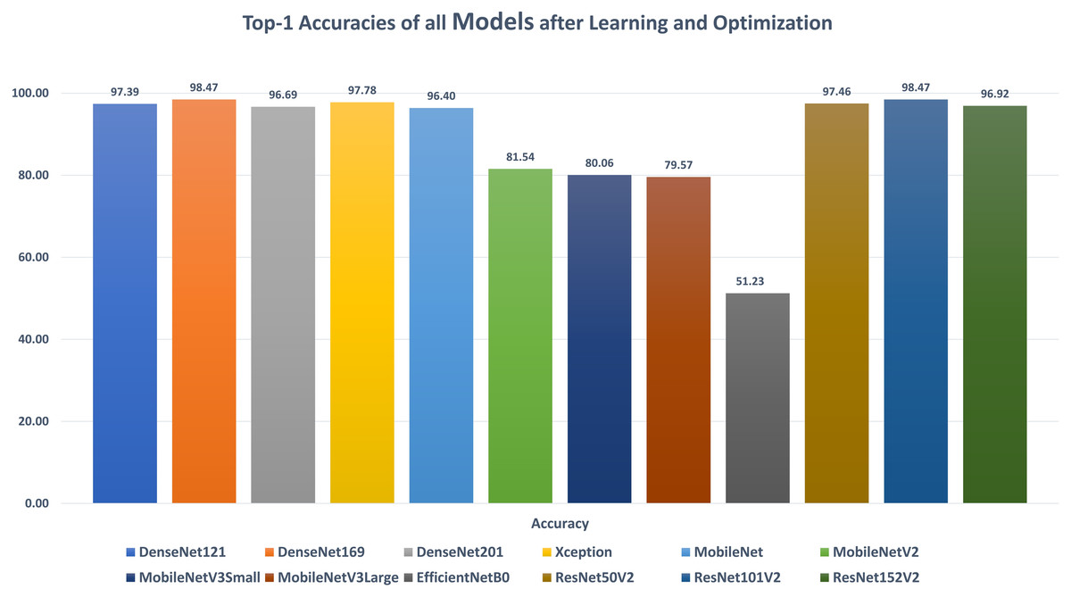
Figure 9: The top-1 accuracies of all reported experiments.
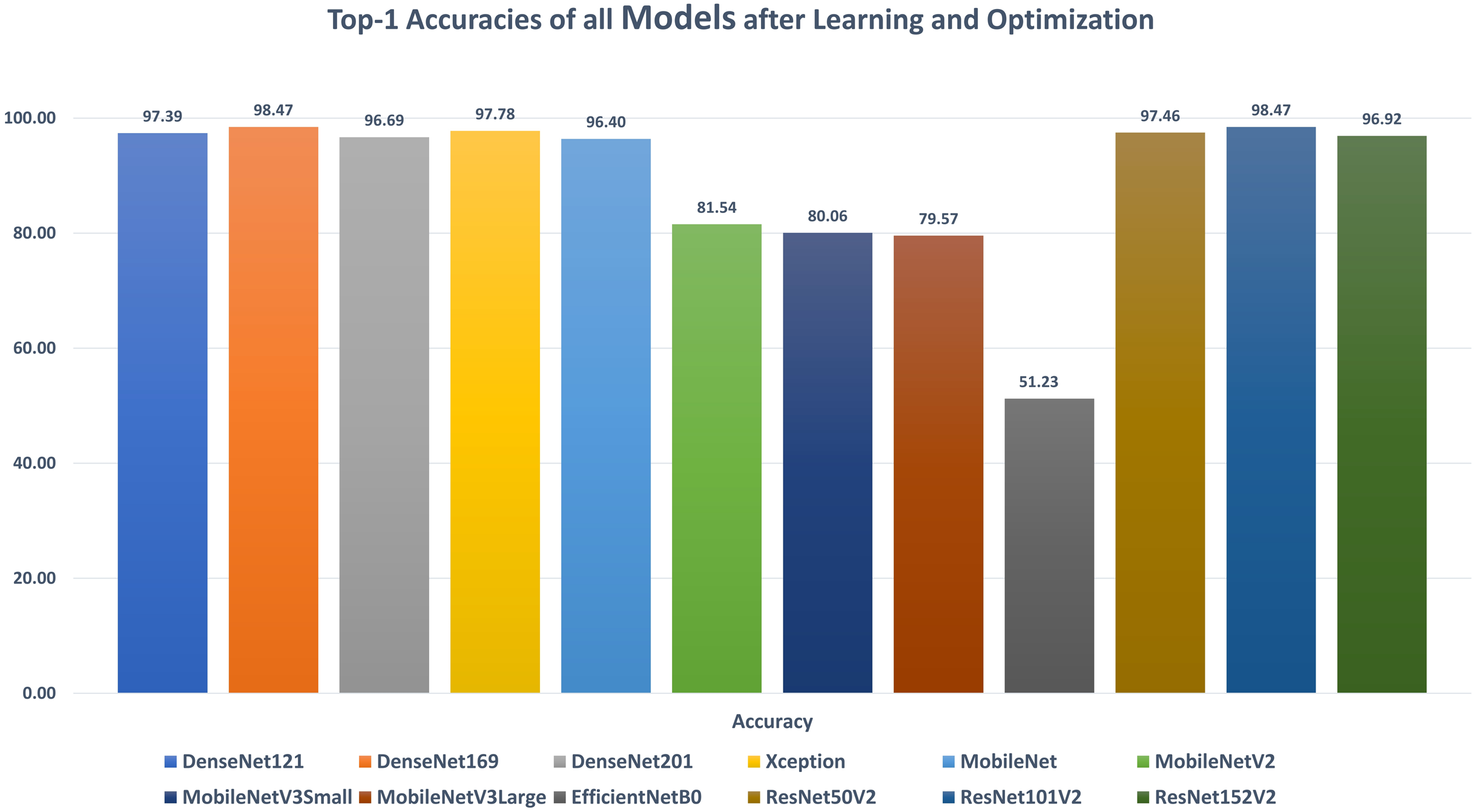
Comparative study
Table 31 shows a comparison between the results of both the proposed OTLD-COVID-19 technique and the other state-of-the-art techniques. The techniques are ordered according to the year of publication. The recorded results show that the proposed OTLD-COVID-19 technique outperforms the four classes’ state-of-the-art compared techniques. Figure 10 depicts a delta comparison between the current study and related works concerning the accuracy. It shows that the current study accuracy exceeds 11 related works accuracies.
| Research | Classes # | Accuracy | Sensitivity | Specificity | Precision | F1-Score | AUC | Recall |
|---|---|---|---|---|---|---|---|---|
| Mukherjee et al. (2020) | 2 | 96.92% | 94.20% | 100.0% | 100.0% | 97.01% | 99.22% | N/A |
| Wang, Lin & Wong (2020) | 3 | 92.40% | 80.00% | N/A | 88.90% | N/A | N/A | N./A |
| Majeed et al. (2020) | 4 | N/A | 94.52% | 99.35% | N/A | N/A | N/A | N/A |
| Hammoudi et al. (2020) | 2 | 96.28% | 97.90% | N/A | 94.80% | N/A | N/A | N/A |
| Hussain et al. (2021) | 4 | 91.20% | 91.76% | 93.48% | 92.04% | 90.04% | N/A | 91.90% |
| Farooq & Hafeez (2020) | 4 | 96.23% | 100.0% | 100.0% | N/A | 100.0% | N/A | N/A |
| Apostolopoulos & Mpesiana (2020) | 3 | 96.78% | 98.66% | 96.46% | N/A | N/A | N/A | N/A |
| Narin, Kaya & Pamuk (2020) | 2 | 98.00% | 96.00% | 100.0% | 100.0% | 98.00% | 100.0% | N/A |
| Islam et al. (2020) | 2 | 96.10% | N/A | N/A | N/A | N/A | N/A | N/A |
| Nayak et al. (2021) | 2 | 89.33% | 100.0% | N/A | N/A | N/A | N/A | N/A |
| Khan, Shah & Bhat (2020) | 4 | 89.60% | N/A | 97.90% | 93.17% | 95.61% | N/A | 98.25% |
| Islam, Islam & Asraf (2020) | 3 | 99.40% | 99.30% | 99.20% | N/A | 98.90% | 99.90% | N/A |
| Aslan et al. (2021) | 3 | 98.70% | N/A | 99.30% | N/A | 98.80% | 99.00% | 98.80% |
| Sethy et al. (2020) | 3 | 95.33% | 95.33% | N/A | N/A | 95.34% | N/A | N/A |
| OTLD-COVID-19 Approach | 4 | 98.47% | 98.47% | 99.50% | 98.50% | 98.49% | 99.83% | 98.47% |

Figure 10: A delta comparison between the current study and related works.
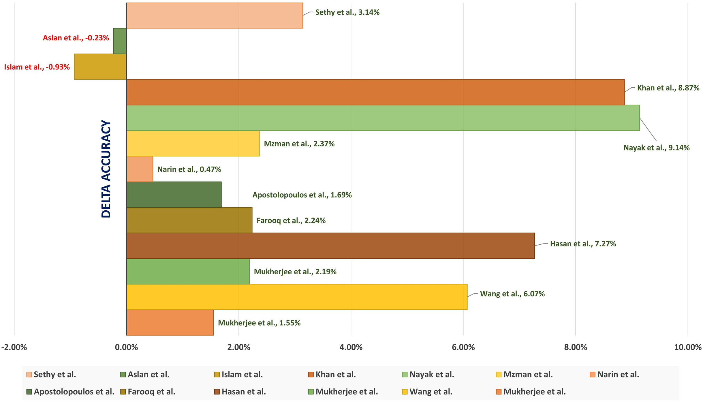
Conclusion
Early detection of COVID-19 positive cases is essential to prevent the spread of this pandemic and treat affected patients quickly. This study presented an Optimized Transfer Learning-based Approach for Automatic Detection of COVID-19 (OTLD-COVID-19) approach, which adopted the Manta Ray Foraging Optimization (MRFO) algorithm to optimize the parameters and hyperparameters of twelve off-the-shelf CNN architectures. The proposed OTLD-COVID-19 approach aims to aid the radiologists in automating the classification of COVID-19 cases based on chest X-ray images. The OTLD-COVID-19 approach is built upon five essential phases. A four-class real dataset has been constructed from eight public datasets to get a relatively large number of chest X-ray images (=12,933 images). Besides, data augmentation is performed to increase the size of the training set and enhance generalization. The training and testing ratio of the dataset was set as 85% and 15%, respectively. The obtained experimental results showed that the proposed OTLD-COVID-19 approach achieved high-performance metrics that outperformed the compared approaches. To extend this work, Generative Adversarial Networks (GAN) can supplement the lack of training set to improve the performance of the classification process. In expansion, the number of other diseases causing pneumonia may be expanded, and the proposed approach can be utilized to distinguish them from the COVID-19. This study could also be extended to other diseases to help the healthcare system respond more effectively during any possible future pandemic.