Analysis of a Model for Coronavirus Spread


1
Laboratory of Biomathematics, Univ. Sidi Bel Abbes, P.B. 89, Sidi Bel Abbes 22000, Algeria
2
Dipartimento di Matematica “Giuseppe Peano”, Università di Torino, via Carlo Alberto 10, 10123 Torino, Italy
*
Author to whom correspondence should be addressed.
†
Member of the INdAM research group GNCS.
Mathematics 2020, 8(5), 820; https://doi.org/10.3390/math8050820
Submission received: 3 April 2020
/
Revised: 14 May 2020
/
Accepted: 15 May 2020
/
Published: 19 May 2020
(This article belongs to the Special Issue Mathematical and Numerical Analysis of Nonlinear Evolution Equations : Advances and Perspectives)
Abstract
:The spread of epidemics has always threatened humanity. In the present circumstance of the Coronavirus pandemic, a mathematical model is considered. It is formulated via a compartmental dynamical system. Its equilibria are investigated for local stability. Global stability is established for the disease-free point. The allowed steady states are an unlikely symptomatic-infected-free point, which must still be considered endemic due to the presence of asymptomatic individuals; and the disease-free and the full endemic equilibria. A transcritical bifurcation is shown to exist among them, preventing bistability. The disease basic reproduction number is calculated. Simulations show that contact restrictive measures are able to delay the epidemic’s outbreak, if taken at a very early stage. However, if lifted too early, they could become ineffective. In particular, an intermittent lock-down policy could be implemented, with the advantage of spreading the epidemics over a longer timespan, thereby reducing the sudden burden on hospitals.
MSC:
92D30; 92D251. Introduction
The coronavirus infection has been spreading for a few months. Authorities in several countries have relied on scientific tools for fighting the epidemics. With the lack of a vaccine, distancing methods have been forced on populations to avoid the transmission by direct contact. In laboratories, possible vaccines are being developed, but at the moment they are still at the experimental stage [1]. Meanwhile several models, mathematical, statistical and computer-science-based, are being developed to study the disease and contribute to fighting it.
Models for the spread of epidemics are classic, and an excellent presentation is [2]. In general, the total population is partitioned into at least two classes, susceptibles and infectives, with migrations from the former to the latter by disease propagation through direct or indirect contact, if the disease is transmissible. Additionally, if it can be overcome but causes relapses, the infected can become susceptible again, after maybe going through an intermediate class of being recovered. More sophisticated versions include quarantined and exposed individuals. Some of these classes will be considered also in the present study and illustrated in detail before the model formulation process.
In [3] the disease evolution forecast in several of the most affected countries is attempted, using for that purpose, parameter estimation techniques to calibrate the model. The involved compartments are susceptibles, asymptomatic individuals and symptomatic ones, which in turn are partitioned into reported and unreported cases. In [4] a simple SIRI model is considered, in which the recovered could still contribute to the disease spreading. The model is then extended to account for a possible vaccine, which, unfortunately, at present is not yet available, although several laboratories worldwide are trying to develop and test it, as mentioned above. In [5] a dynamic model for the diffusion of Covid-19 has been proposed. The transmission network is made by the bats–hosts–reservoir–people compartments; compare also [1]. As it amounts to about 14 differential equations and 25 parameters, it is rather complex. From it, the authors have obtained a simplified version, consisting of six compartments and 13 parameters. Then, the disease basic reproduction number has been calculated.
Our aim here is the mathematical analysis of a slightly modified version of the simpler model in [5]. The most important change accounts for the fact that asymptomatic people may indeed turn into fully symptomatic and infectious individuals. This feature also distinguishes the system introduced here from the one studied in [6], which, however, contains more compartments. The main aim of that study is the forecast of the epidemic spread in various cities in China, considering, additionally, weather data, which finally indicate that higher humidity favors the containment of a coronavirus epidemic. Our focus in the first part of this investigation is the theoretical analysis of the proposed system, and then we perform some preliminary simulations with realistic parameter values. More extended simulations will be devoted to a subsequent study.
The analysis of dynamical systems usually considers the possible equilibria that can be attained, assessing their feasibility and stability, and possible connections between them. For more details on these issues we refer the reader to classical texts, such as [7,8,9].
The paper is organized as follows. The main findings are outlined in the next section, which also discusses the results of numerical simulations. Section 3 contains an evaluation of their implications under various distancing policies. We formulate the model in Section 4, where we also analyze it mathematically, showing boundedness of the trajectories, establishing an expression for the disease basic reproduction number, finding its equilibria and assessing their local stability, and global stability is established just for the disease-free equilibrium. The section ends with the details on the numerical simulations.
2. Results
2.1. Theoretical Findings
The main analytical findings of this investigation are summarized in Table 1 and Table 2. The expressions of , , , and are given by Equations (3) and (6).
The model (1) allows only three possible equilibria; the disease-free state , where only susceptibles thrive; an equilibrium without symptomatic infected, which occurs only for a very particular case, when the exposed individuals become all asymptomatic infected; and finally, the endemic equilibrium . All these equilibria are locally asymptotically stable, if suitable, rather complicated conditions, hold. Among the endemic and the disease-free equilibrium bistability is impossible, since they are related via a transcritical bifurcation.
2.2. Simulations Results
We have performed some simulations with the parameter values listed in Table 3, to simulate various implementations of the distancing policy, which actually is in current use in several countries. The simulations may not be fully realistic, but our point is to investigate their qualitative behavior, not to give quantitative forecasts.
We look at the influence that the time of starting the restrictive measures has on the disease spread, while keeping fixed the time of their lifting. We next investigate the effect of the time at which the restricting measures are lifted.
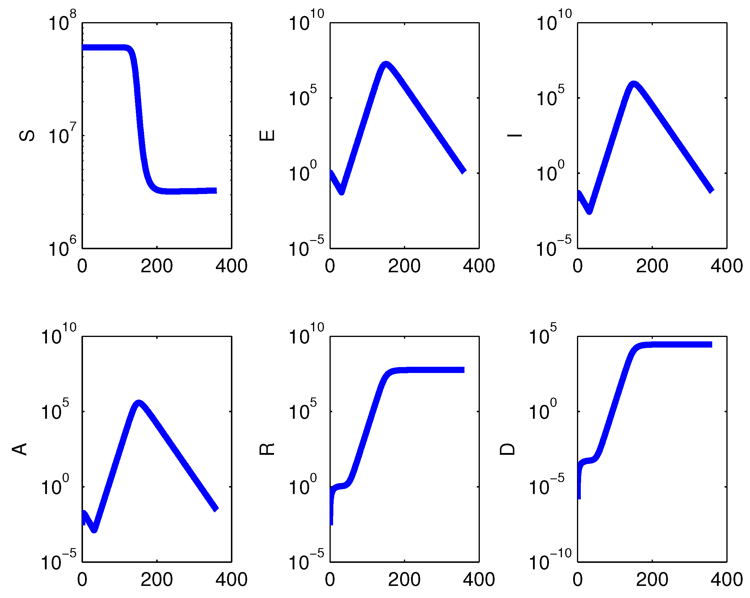
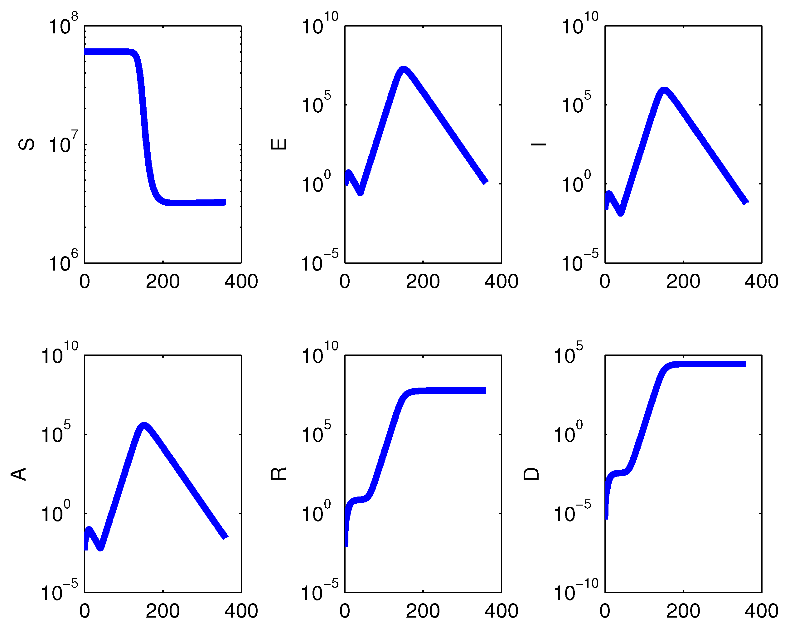
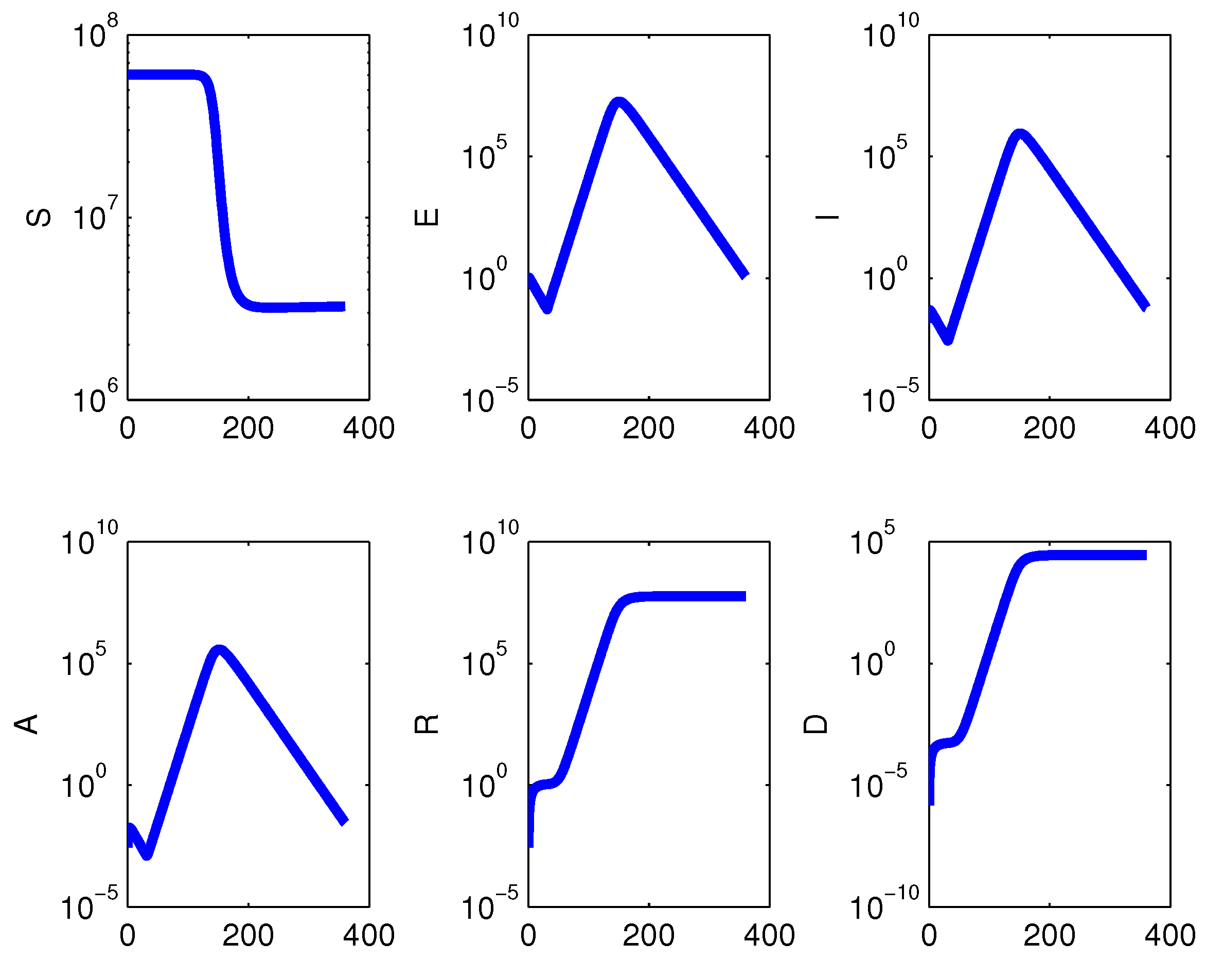
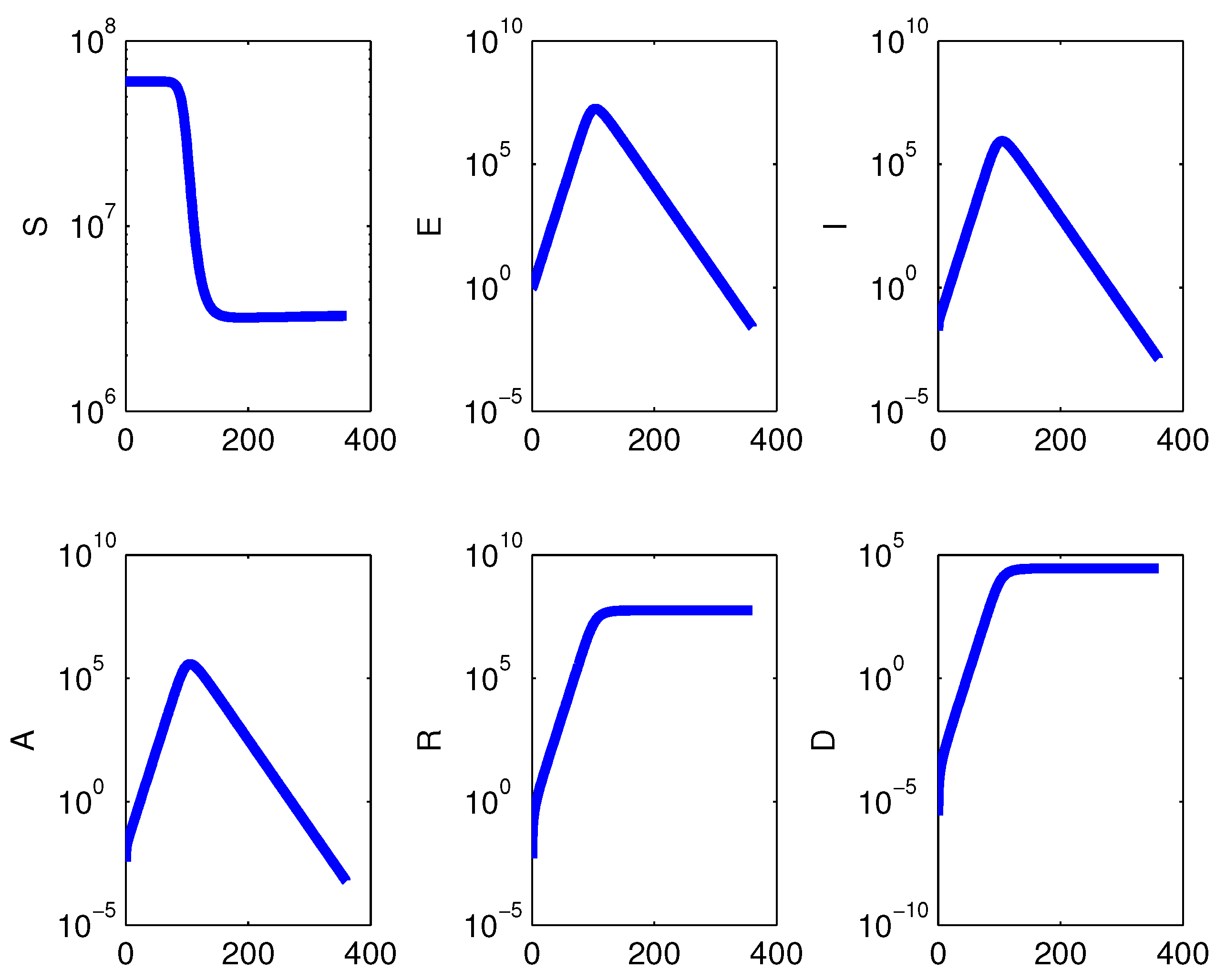
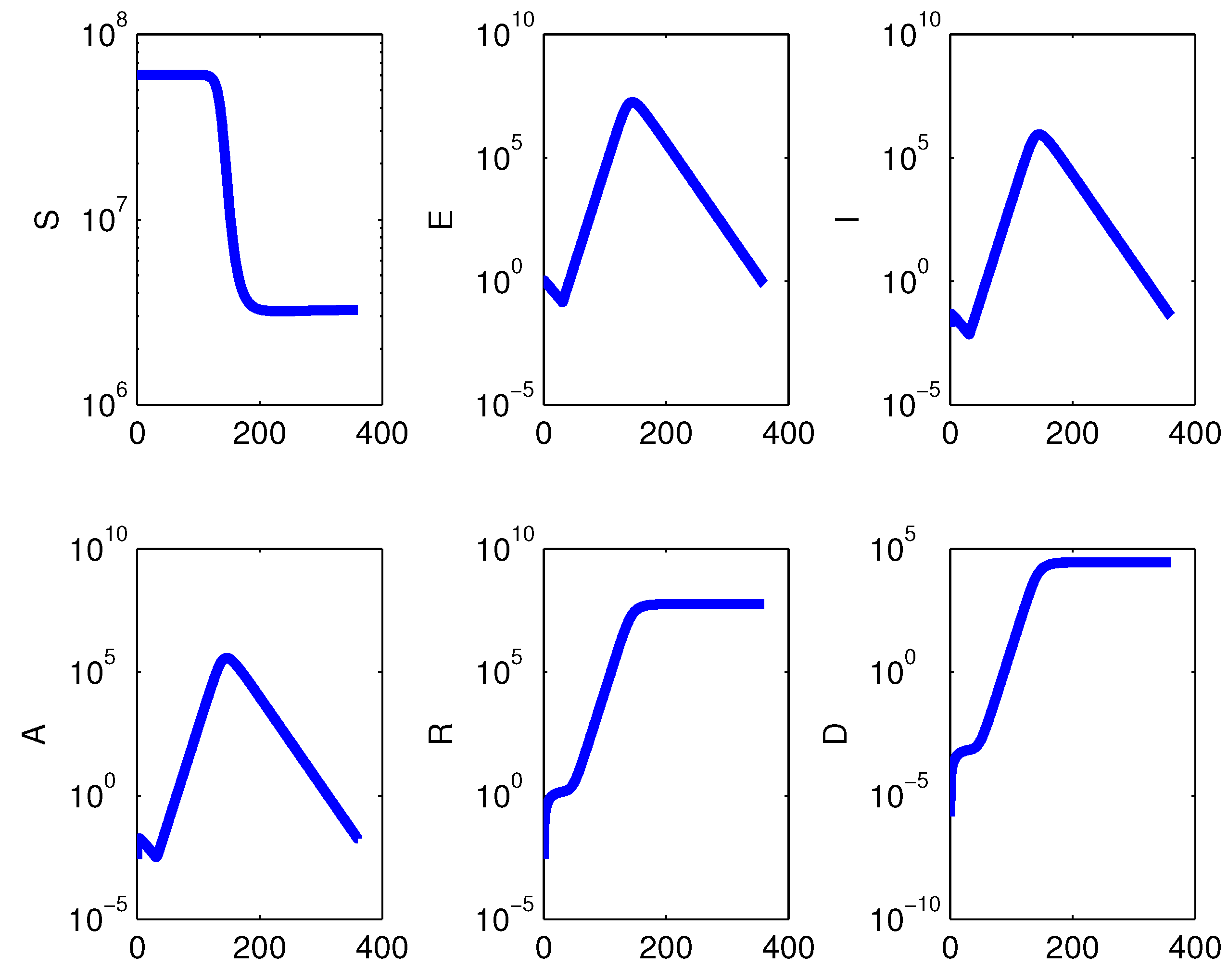
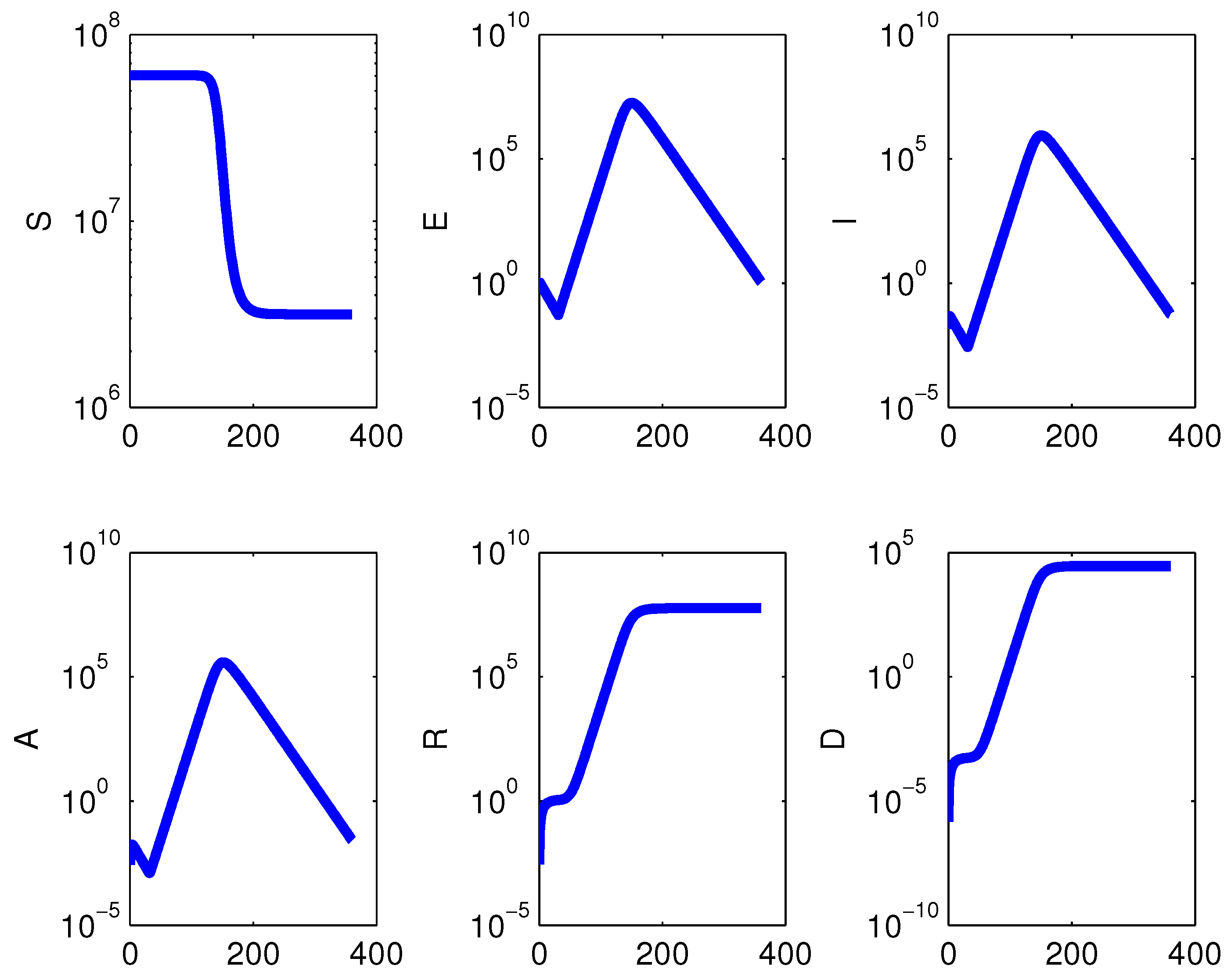
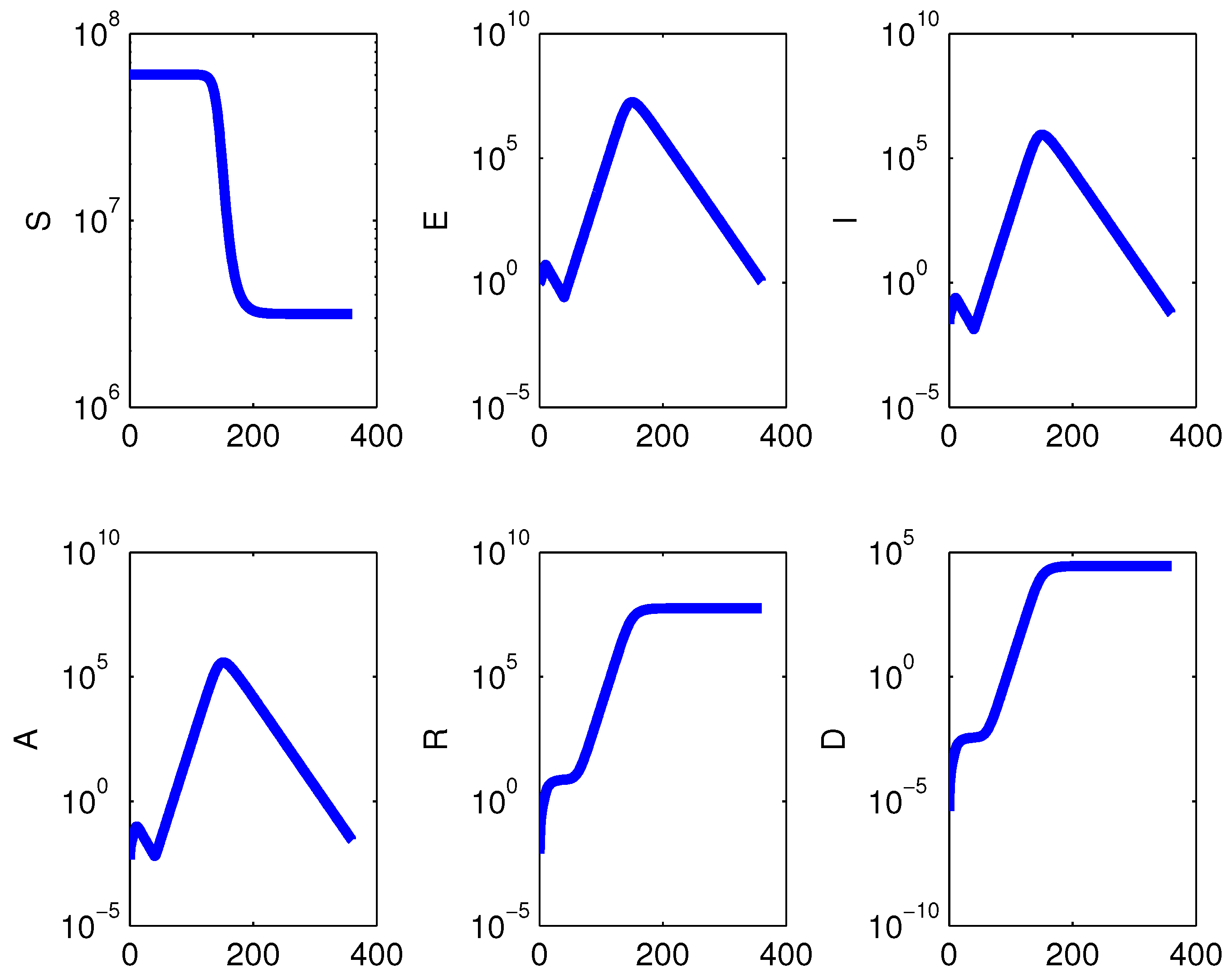
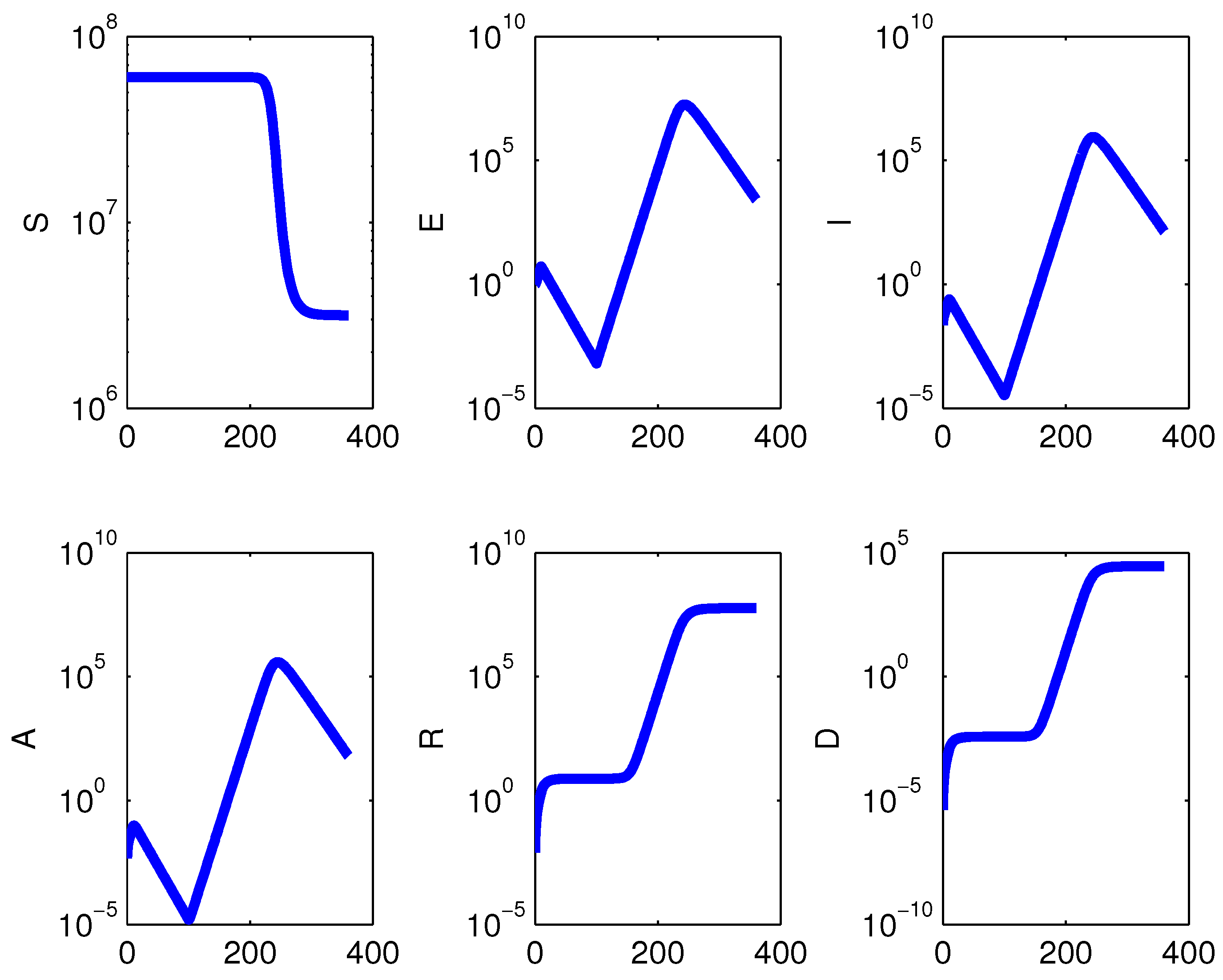
Now comparing the results for the start of implementation at and , and ending them at the same time, it is seen that the earlier the measures are taken, the better it is, because the epidemic’s outbreak is kept in check. In Figure 1 the epidemic outbreak starts around time 30, immediately after lifting the restrictions, while in Figure 2 the initial surge before the measures are implemented is damped by their implementation, and after their lifting the outbreak occurs. Both figures use . The same result is seen using as the time for removing the restrictions; compare Figure 3 and Figure 4. In Figure 3 nothing apparently happens until time 100 because of the restrictions. When they are lifted, the epidemic spreads. In Figure 4 there is a small peak at the onset of the contagion, immediately curbed by the containment measures, lasting as long as they are in use. In spite of their longer implementation, the outbreak occurs nevertheless with the peak at the same time as in Figure 3.
The investigation of different timings for introducing and relaxing the distancing measures shows that a late implementation has no effect, as the peak of the epidemic occurs and then these measures are ineffective, independently of how long they are implemented. An earlier implementation followed by their subsequent lifting leads to a secondary peak at some time later, the occurrence of which seems to be related to the time for which the measures are implemented; the longer the latter, the longer the delay in the secondary outbreak. However, the number of affected people remains the same.
Unfortunately, the result of the simulations indicates that essentially the whole population gets affected by the disease. Only the timings differ, if distancing measures are taken.
Thus, if the measures are implemented too late, independently of the time at which they are removed, the outbreak occurs and their subsequent application becomes, therefore, irrelevant, as it cannot be kept in check any longer; compare Figure 2 and Figure 4. On the other hand, by implementing them at the early stages of the contagion process, the outbreak can be delayed, as long as these measures are implemented, as can be seen from Figure 1 and Figure 3. If they are lifted, the final results of the epidemic’s outbreak are essentially the same as if they were not at all implemented, in terms of the number of people being affected by the disease and with possible ultimate fatal consequences; compare the peaks of all the infected classes in Figure 1, Figure 2, Figure 3, Figure 4 and Figure 5 also with the results in Figure 6 where no measures are taken to prevent the epidemic from spreading.
An intermittent lock-down policy, simulated as an alternative way of coping with the outbreak, might be important to render the burden on hospitalizations smaller, as it tends to spread the epidemic over a longer timespan.
For the particular situation in Italy, note that patient number 1 was diagnosed on 21 February, and the distancing measures in the area were in place starting the following days up to about two weeks later, and then extended to the whole country. Incidentally, patient number 0, the initial carrier of the disease, has never been identified, although there are some speculations. However, in the current news, it is reported that the virus was already circulating yet not known of in Northern Italy in January, which means that additional time had elapsed before the restrictions were applied.
Thus, apparently, these results are negative as for the possibility of containing the spread in the long run, in line with what is hinted in [10], with the exception of the intermittent distancing measures policy, which may spread the epidemic’s effects over longer timespans. However, there are some assumptions in the model that make it too crude, so that we plan a deeper subsequent study. In particular, here the results depend on homogeneous mixing, which for a large country is hardly the case. Secondly, this is a continuous model, for which the compartments are depleted only asymptotically. Thus it is not possible to prevent the class of infectives from vanishing in finite time, so that even a small residual in it would start the epidemic’s outbreak again. Therefore the somewhat negative results obtained might hopefully be better off in practice. Suitable modifications of the model along these lines will be the subject of a further investigation.
3. Discussion
We have investigated a simple model for the coronavirus pandemic. The steady states, apart from a symptomatic-infected-free point, which is unlikely to exist, are the disease-free equilibrium and the endemic state. The model differs from other current models that are being studied for a few features. From the simplified model that appears in [5], because our formulation contains less equations, it does not consider the viruses compartment, and above all, we allow disease-related mortality, which apparently is missing in the cited paper. Furthermore, we allow the progression of asymptomatic individuals to the class of fully symptomatic. This feature certainly distinguishes it also from [6], where asymptomatics recover or become diagnosed with the disease, but do not spread it any longer. In the present situation in Italy our assumption is very realistic.
There is no possibility of bistability in our situation, as the two fully meaningful equilibria are related to each other via a transcritical bifurcation. The disease-free equilibrium is also globally asymptotically stable, if it is locally asymptotically stable. An expression for the basic reproduction number is established, with a possibly realistic numerical value [11,12].
The simulations show that containment measures could be effective in delaying the epidemic’s outbreaks if taken at a very early stage, but when lifted the outbreaks would occur anyway and affect almost the whole population. However, this last statement should be mitigated by the drawbacks inherent in the model’s assumptions, as mentioned in the previous section, thereby leaving hope that in practice it will not occur, if the measures are properly implemented.
We next discuss in detail the various different restriction policies that we have simulated.
3.1. Epidemic with a Lock-Down
In this case, in particular, assuming for the disease transmission coefficient the reference value , we reduce it to during the interval and reinstate the standard value afterwards; we monitor the epidemic’s evolution over six months. Figure 1, Figure 2, Figure 3, Figure 4 and Figure 5 show the results of different choices for and . Containment measures are effective as long as they are implemented, if they are taken early enough, before the epidemic attains its peak.
Since reducing the transmission by one order of magnitude means that to infect a susceptible with rate , it is necessary for only one infected; with , 10 infected would be necessary. Thus since the lock-down is not perfect, as for instance, some essential activities like food production are still going on, a hypothetical reasonable estimate for the contact reduction is three orders of magnitude. A comparison with a different, milder reduction, is made, showing essentially no difference in the results, see Figure 7.
3.2. Epidemic with Total Isolation
We changed also the policy to an improbable absolute confinement of every individual in the population, reducing the transmission to exactly zero. The results show no change with respect to those of the lock-down policy. We report only Figure 5, which is identical to Figure 1. The same occurs in the cases contemplated by Figure 2, Figure 3 and Figure 4.
3.3. The Simplified No-Demographics Model
We repeated the simulations for the model (1) in which we set . In the simulations we observed some small changes in the susceptibles behavior, with respect to the full model with vital dynamics. Figure 8 and Figure 9 are the counterparts of the Figure 1 and Figure 2. The ultimate impact of the epidemic is essentially the same; compare in particular, the curves of recovered and deceased. For the total isolation case, Figure 10 shows the same features; compare it with Figure 5. Similar considerations hold for the various remaining cases, and therefore, the pictures are not reported.
3.4. Investigation of Different Timings for Restrictions’ Introduction and Lifting
A further study has been carried out to assess the impact of the time until taking action on the containment measures. All the possible different combinations of simple restriction or total isolation as well as the presence or the absence of demographic effects give essentially the same results. Therefore we present only the results for some selected alternatives, giving the plots in semilogarithmic or total population values, but stressing that for the options not considered, the figures would be the same.
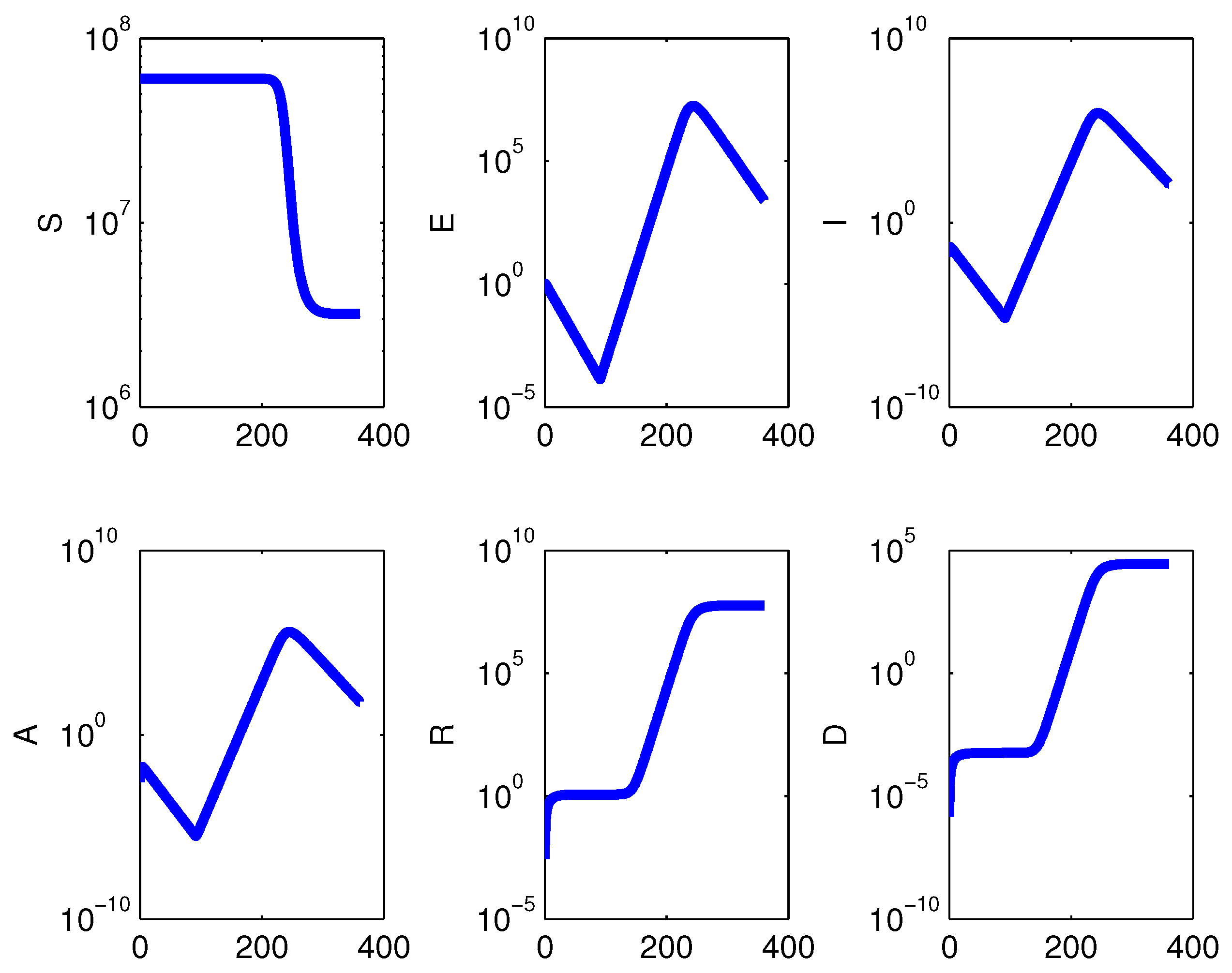
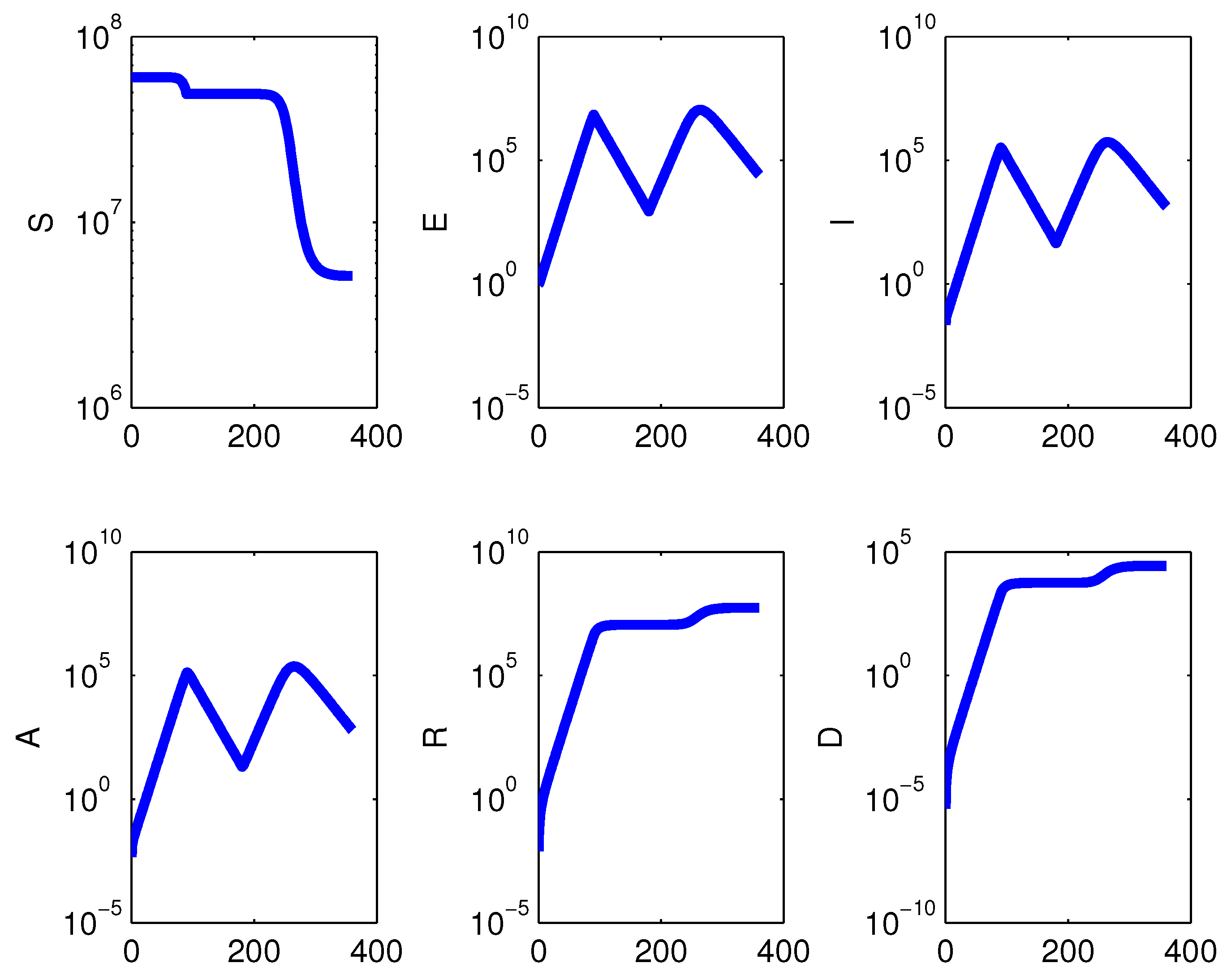
In case the first restriction measure is taken too late, specifically at time , and followed by lifting it either one month or three months later, the epidemic occurs and the measures have no effect whatsoever; see Figure 11, where measures are kept for three months.
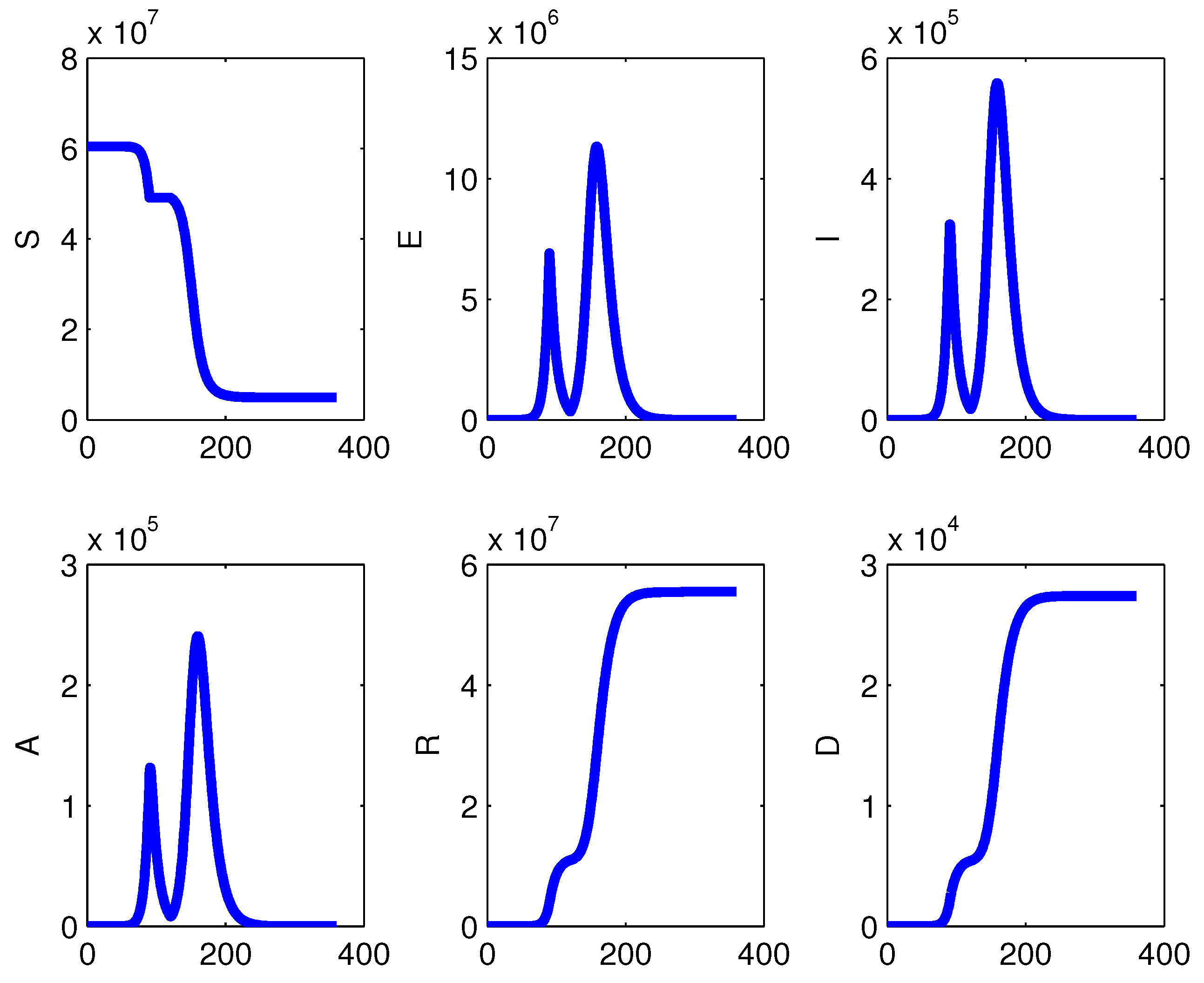
Beginning the restrictions after three months from the start of the epidemic and removing them one month afterwards, causes a second peak about two months later; i.e., six months after the onset of the disease spreading (Figure 12), with a higher number of affected individuals. If instead the lock-down is implemented for three months, the second peak is delayed further, occurring about three months later, Figure 13. Although the pictures are shown on different population scales, absolute values and semilogarithmic, a comparison of the heights of the peaks for the various types of infected subpopulations indicates no difference. Hence, these policies cannot significantly influence the number of people ultimately affected by the disease.
3.5. The Intermittent Lock-Down Policy
We finally simulated a policy that attempts to assess the number of infectives at regular times, with a of period one week. If they exceed a threshold, taken to be 10, the lock-down is implemented for a week, and then lifted. Figure 14 and Figure 15 show the results for the case with vital dynamics and in the case of . Note that susceptibles in both cases are at a constant value, the vertical scale being extremely small. The infected are kept below the threshold, and the periodic recurrences of the epidemic somewhat change its final impact, as the curves of recovered are reduced by about two orders of magnitude, and above all, the ones of the deceased decrease by about four orders, with respect to the ones found with the one-time lock-down policy. The other relevant change is that here the phenomenon is observed over a longer timespan. Thus the cumulative effects are spread out over a much longer time. This will have some importance to lessening the burden on hospitals. Figure 16 shows the results if the check policy starts immediately at time 1 rather than after a week.
Comparing the population values with the intermittent policy with the one time lock-down, done early enough and implemented for one month, the final outcomes are milder than the latter. Thus the intermittency allows the control of the outbreaks. Susceptibles are almost depleted in the one-time policy; with the intermittent one, however, they are essentially spared from getting the disease; compare Figure 17 and Figure 18.
The intermittency has also been checked with different time intervals. Comparing Figure 19, Figure 20, Figure 21 and Figure 22, it is seen that the more frequent the checks are implemented, the lower are the peaks in the exposed class, which in turn leads to a smaller cumulative number of recovered and fatalities, at least comparing the policies for the one- and two-weeks alternatives, Figure 19 and Figure 20. For the longer intervals between the checks, again the peaks are higher, the longer the timespan, but it is observed that as time elapses, their heights tend to decrease; see Figure 21 and Figure 22.
4. Materials and Methods
Here we develop a mathematical model of coronavirus, which is a zoonotic disease. Its biological characteristics indicate that the virus transmission occurred first from infected animals to humans [5], and then spread among populations worldwide by contact with infected individuals, to make it a pandemic.
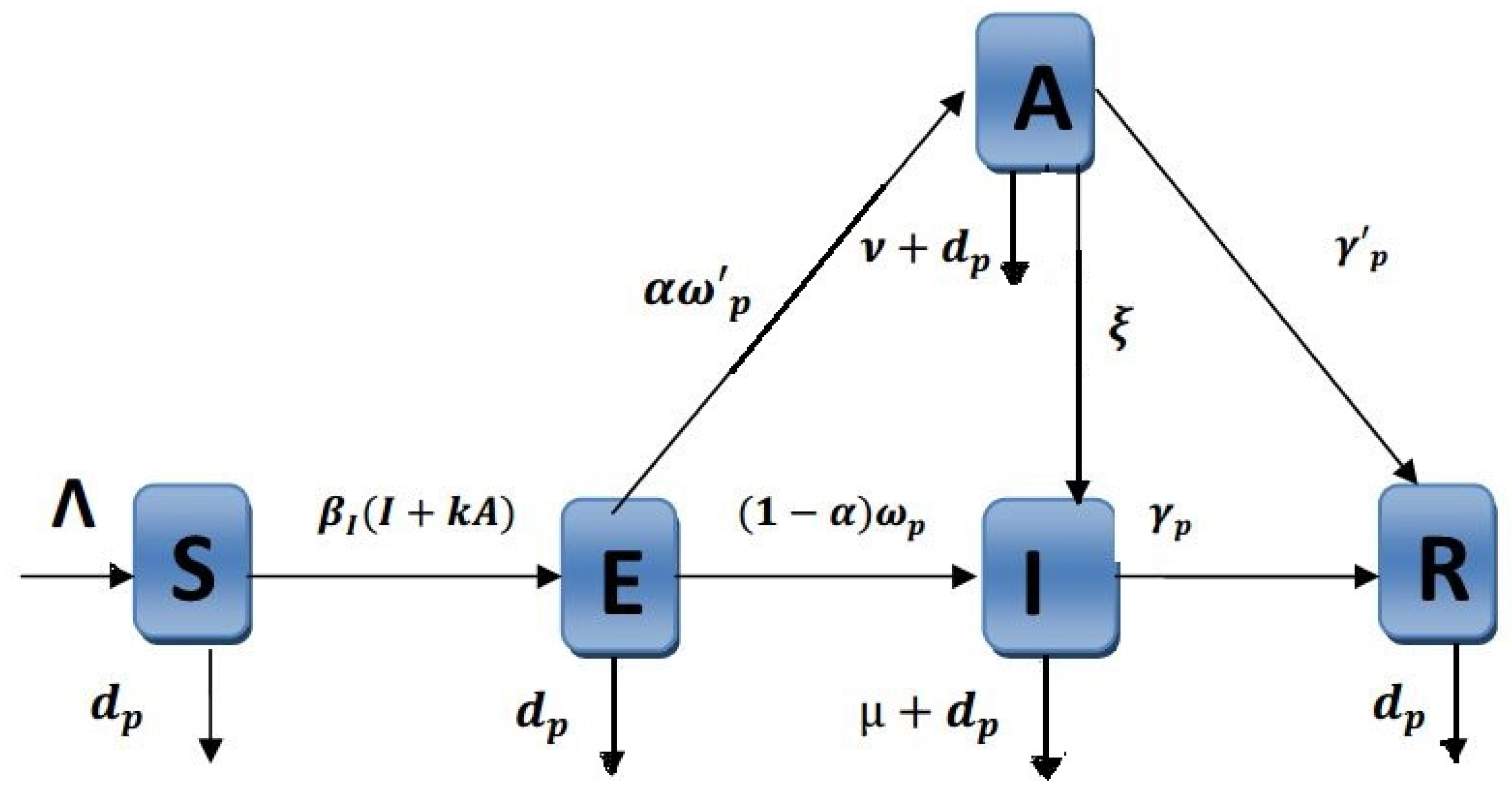
Let denote the total population. It is partitioned into the following five disjoint classes of individuals:
: The susceptible class, the individuals who have not yet been exposed to the virus.
: The exposed class, describing people who have become in contact with the virus, but are in incubation period and not yet able to spread the disease; possible presymptomatic individuals that can transmit the infection [13,14,15] are assumed to have already moved to the asymptomatic class defined below.
: The symptomatic infectious class, individuals that manifest symptoms and can spread the disease.
: The asymptomatic infectious class; those persons that can spread the disease even without having explicit symptoms.
: The removed class, that includes the people that recovered from the disease.
Thus, .
The basic mechanisms underlying the model are shown in Figure 23. The model is formulated taking into account all the possible interactions among the compartments that were described above.
Under the quasi-steady-state assumption of the total human population, we impose that susceptible individuals are recruited at the constant rate , become infected by direct contact with an infectious individual at rate , which is scaled by a factor k to account for the possibility that the latter is asymptomatic. Finally, all human individuals are subject to natural mortality . These considerations are incorporated in the first equation of the system (1).
Individuals that contract the disease are accounted for in the second equation of (1). They become exposed, i.e., they cannot yet spread the virus, which needs an incubation period within the body of its hosts. In this class enter the susceptibles that were contaminated in the two ways described earlier. People leave it by becoming infectious, and either showing symptoms, thereby migrating into class I, or not, therefore, finding themselves in class A. The progression rates into these two classes are and . Furthermore, we assume that a fraction becomes asymptomatic and instead will manifest symptoms.
The third equation models the symptomatic infectious, recruited from the exposed class at rate as described above. Furthermore, there could be asymptomatic individuals that become symptomatic at rate . They leave this class by either progressing to the recovered class at rate , or dying, naturally or by causes related to the disease at rate .
The asymptomatic individuals modeled in the fourth equation appear from the exposed ones, and leave the class by overcoming the disease at rate , dying naturally or by disease-related causes at rate , or eventually showing the symptoms, for which they migrate into class I.
Recovered individuals are those that have healed from the disease. They are subject only to natural mortality. We assume that they have also become immune so that they are unaffected if become in contact with the infectious.
Note that in the simulations also the cumulative class of disease-related deceased people is shown, although the dead are not explicitly accounted for in the model. They indeed represent a sink, and thus do not contribute to the disease propagation. Incidentally, instead, in cultures where the deceased are kept for a while before burial and become in contact with the relatives, it may be necessary to introduce this class in the model, as another potential source of infection.
Taking into account the above considerations, the model dynamics is regulated by the following system of nonlinear ordinary differential equations:
or alternatively, excluding completely the demographic features, by setting and in (1). All the parameters are nonnegative and their meaning is summarized in Table 4. Note that in view of the definitions,
represent respectively the incubation period before manifesting symptoms, the latent period before becoming asymptomatic infectious, the infectious period for symptomatic infection and the infectious period for asymptomatic infection.
Theorem 1.
The system trajectories are bounded. Letting
the set
represents their ultimate attractor. In particular, if , .
Proof.
From the system (1) it follows that the total population evolves as follows:
Solving the differential inequality easily gives
so that all subpopulations, being nonnegative, are bounded as well. □
Note that is positively invariant since all solutions of system (1) originating in remain there for all , in view of the existence and uniqueness of its solutions.
4.1. System’s Equilibria Assessment
The equilibrium points of the model are obtained by equating the right hand side of system (1) to zero. The solution of the so-obtained algebraic system gives three equilibrium points: the coronavirus-free equilibrium , the coronavirus-symptomatic-infected-free equilibrium with conditions and , and the fully coronavirus endemic equilibrium when either or . Specifically, for the former two we have:
where
The feasibility conditions for are
For the fully endemic equilibrium we find
with feasibility condition
4.2. The Basic Reproduction Number
The basic reproduction number for system (1) is found using the next generation matrix method [16]. The reduced system of (1) may be written in compact form as: where
The Jacobian matrices of and at the disease-free equilibrium point are
and
We find that
The next generation matrix is
Thus
We have the following theorem
Theorem 2.
System (1) has the following equilibria:
- 1.
- The coronavirus-free equilibrium which exists always.
- 2.
- In addition, if then system (1) admits another nontrivial equilibrium, in fact:When and , it is the coronavirus-symptomatic-infected-free equilibrium .When either or , it is the fully coronavirus endemic equilibrium .
4.3. System’s Equilibria Stability
4.3.1. Local Stability
In this subsection we investigate the local stability of the system’s equilibria.
Theorem 3.
Letting
Proof.
The Jacobian matrix of system (1) at the coronavirus-free equilibrium is:
At point , the eigenvalues of J are of multiplicity order two and the roots of the following characteristic polynomial of a three by three submatrix of J whose coefficients , are given in (7):
Thus, , and .
Since we can deduce the stability of the coronavirus symptomatic infected-free equilibrium from the stability of the coronavirus endemic equilibrium simply by taking and in the latter, we now just analyze the coronavirus endemic equilibrium .
Theorem 4.
Let
The coronavirus endemic equilibrium is locally asymptotically stable if
Proof.
The Jacobian matrix of system (1) at the coronavirus endemic equilibrium is:
At point , the eigenvalues of J are and the roots of the characteristic polynomial of a three by three submatrix of J. The characteristic equation, in which the coefficients , are given in (10), is:
From Theorem 4 the following result is reached.
Theorem 5.
Let
The coronavirus symptomatic-infected-free equilibrium of the system (1) is locally asymptotically stable if
Proof.
The result can easily obtained from Theorem 4 by taking and . □
Additionally, from the previous discussion, we can claim the following result:
Theorem 6.
There is a transcritical bifurcation between and .
4.3.2. Global Stability
Next, we address the issue of global stability of the coronavirus–free equilibrium, employing as a tool a suitably constructed Lyapunov function and La Salle’s Invariance Principle.
Theorem 7.
The coronavirus-free equilibrium of model (1) is globally asymptotically stable if
Proof.
First, the four equations of (1) are independent of R, therefore, the last equation of (1) can be omitted without loss of generality. Hence, let us consider the following function:
It is easily seen that the above function is nonnegative and also if and only if , , and . Further, calculating the time derivative of P along the positive solutions of (1), we find:
From condition (15) we can show that the coefficients of the term in the last equality are negative. Further, we have for all . Thus, we have for all and if and only if . Thus, the only invariant set contained in is . Hence, La Salle’s theorem implies convergence of the solutions to . From the last equation if (1) we can show obviously that R converge also to 0. Therefore is globally asymptotically stable if . □
4.4. Numerical Simulations
The calculation of the value of according to (6) with the parameter values used in the numerical simulations gives , in line with the current estimates [11,12].
4.4.1. Simulations Methodology
We use a simple own-developed driver code calling the Matlab intrinsic routine ode45, implementing the classical Runge–Kutta 45 integration method for ordinary differential equations.
At first, we consider only the demographic simulation and show that the population is essentially at the same level during a year. This fact is substantiated also by the simulation results, for which there is scant difference between those of the model (1) and the ones obtained by using its no-demographic counterpart, where and are both set to zero.
We then perform three sets of simulations describing different possible scenarios. The first one considers lock-down, i.e., decreasing the contact rate significantly, but not to zero, as some essential activities are still open. Then the total isolation policy, for which the contact rate is set to zero. Finally an intermittent closure policy, for which when infectives reappear in a significant way, temporary lock-down measures resume again.
4.4.2. Data Acquisition
We use data published on official websites about the epidemic’s spread in Italy collected between 29 January and 28 March 2020, a period that spans 61 days, incremented by more recent information [17].
Using the day as the base time unit, we assume that the average incubation period lies in the interval between two and 14 days, with a mean of 8 days. Based on the percentage of the reported symptomatic infected patients, the proportion of symptomatic in the infected class is estimated to be in the interval . The correction k for asymptomatics to diffuse the disease is set in the range . There have been 27,359 deaths between 15 February and 29 April [17], with changes in the number of fatalities every day. Dividing the fatal cases by the timespan, one gets 370 daily fatalities, which gives a rate . Using this value in the simulation, puts the total losses to about . But we observed that apparently children hardly get the disease, the younger and adult people have it generally in a mild form and fatalities occur mainly for the elderly people, compare with Figure 3 of [18]. In view of the fact that there is no age structure in this model, we corrected this value by taking a third of the above result to set the disease mortality rate at the final value , which gives a reasonable estimate for the losses in the timespan, in rough agreement with the actual tallies. We neglect altogether mortality for the asymptomatics, setting . Based on the officially published data we estimate , . For the initial values, the total population is obtained from the report published by the official cite of worldometers [19], . To avoid demographic effects, we set the susceptible recruitment rate in order that on the timespan of the simulation the total population N does not change much.
4.4.3. The Pure Demographic Case
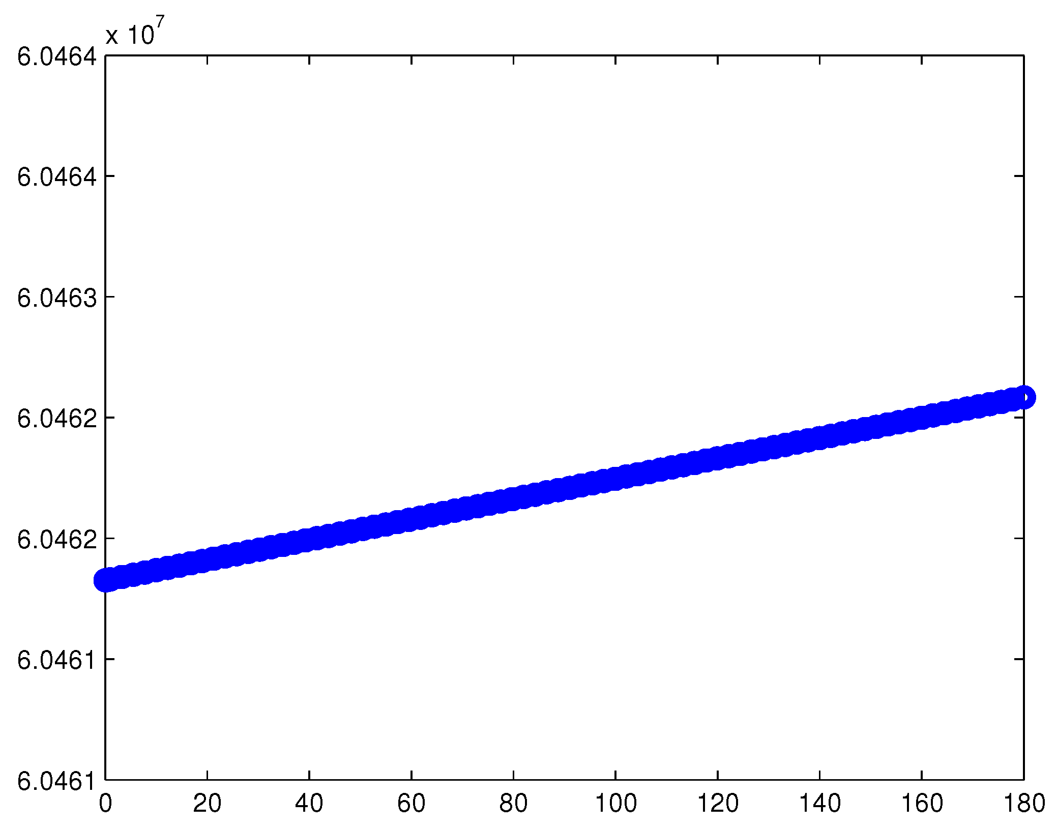
We simulate first the population model without disease. In so doing, we varied the parameter until a satisfactory behavior of N, the total population was found. With there is little variation of N during a whole year, the population remains roughly stable around the level , see Figure 24. In this way the demographic effects are sort of removed, and we can concentrate mainly on the epidemics. Actually, the number of newborns per day in Italy would be about four times higher, but as mentioned, we just would like here to hide the demographics from the simulations and not have a picture more adherent to reality.
4.4.4. Epidemics Spread in the Absence of Measures
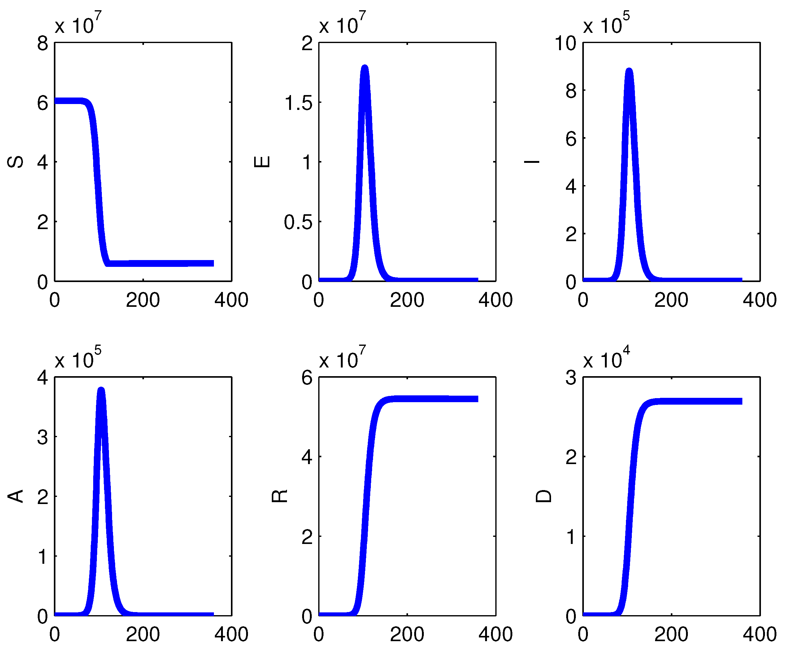
Here we introduced the disease, with incidence . The result is shown in Figure 25 for absolute numbers, and in Figure 6 in semilogarithmic scale. In this case no measures are assumed to be taken to counteract the epidemics. These results are reported in order be able to compare the simulations with restrictions to what would happen if the containment measures were not taken.
4.4.5. Containment Measures for the Epidemics
Finally, we considered the introduction of the distancing policy. It is assumed to start at time and end at time . Two forms of containment measures are considered, substantially reducing the contact rate, or even setting it equal to zero, meaning the extreme measure of total individuals isolation.
In particular, we present the experience of using the reference value of the contact rate , then reducing it to during the interval . We then reset it to its previous reference value after time . We monitored the epidemics evolution over six months.
The alternative, milder choice is also used, for comparison.
The simulations are then repeated with total isolation, setting during the implementation of the restrictions.
A comparison of the results with the model obtained by disregarding the demographic parameters, i.e., setting is also performed in the same way as done for the model (1).
Different timings for taking both the first restriction measure and for lifting it are then investigated, using all the above alternatives.
Finally an intermittent restrictive policy is examined, for which when the infected are observed to trespass a threshold, distancing measures are taken. Here again lock-down or total isolation produce essentially the same results. The use of different timings for the introduction of the restrictions is also scrutinized.
Author Contributions
Model formulation, Y.B. and E.V.; methodology, Y.B., M.H. and E.V.; formal analysis, Y.B., M.H. and E.V.; writing—original draft preparation, Y.B.; simulations, writing—review and editing, E.V. All authors have read and agreed to the published version of the manuscript.
Funding
E.V. was partially funded by the local research project “Questioni attuali di approssimazione numerica e loro applicazioni” of the Dipartimento di Matematica, Universitá di Torino. This research has been undertaken within the framework of the COST Action: CA 16227—Investigation and Mathematical Analysis of Avant-garde Disease Control via Mosquito Nano-Tech-Repellents. This work was partially supported by the Ministry of Higher Education and Scientific Research of Algeria (MESRS) and General Direction of Scientific Research and Technological Development (DGRSDT) through Research Project-University Formation (PRFU: C00L03UN220120190001 and PRFU: C00L03UN220120180004).
Acknowledgments
The authors would like to thank the reviewers for their valuable comments and suggestions that greatly improved the presentation of this work.
Conflicts of Interest
The authors declare no conflict of interest.
References
- Cecconi, M.; Forni, G.; Mantovani, A. COVID-19: An Executive Report, “Commissione Salute, March 25th”; Accademia Nazionale dei Lincei: Roma, Italy, 2020. [Google Scholar]
- Herbert, W. Hethcote, The Mathematics of Infectious Diseases. SIAM Rev. 2000, 42, 599–653. [Google Scholar] [CrossRef] [Green Version]
- Magal, P.; Webb, G. Predicting the number of reported and unreported cases for the COVID-19 epidemic in South Korea, Italy, France and Germany. medRxiv 2020. [Google Scholar] [CrossRef]
- Buonomo, B. Effects of information-dependent vaccination behavior on coronavirus outbreak: Insights from a SIRI model. Ricerche di Matematica 2020. [Google Scholar] [CrossRef] [Green Version]
- Chen, T.M.; Rui, J.; Wang, Q.P.; Zhao, Z.Y.; Cui, J.A.; Yin, L. A mathematical model for simulating the transmission of Wuhan novel Coronavirus. bioRxiv 2020. [Google Scholar] [CrossRef] [Green Version]
- Jia, J.; Ding, J.; Liu, S.; Liao, G.; Li, J.; Duan, B.; Wang, G.; Zhang, R. Modeling the control of Covid-19: Impact of policy interventions and meteorological factors. Electron. J. Differ. Equ. 2020, 2020, 1–24. [Google Scholar]
- Murray, J.D. Mathematical Biology; Springer: Berlin/Heidelberg, Germany, 2002. [Google Scholar]
- Perko, L. Differential Equations and Dynamical Systems; Springer: Berlin/Heidelberg, Germany, 2001. [Google Scholar]
- Strogatz, S. Nonlinear Dynamics and Chaos; Perseus Books: Reading, MA, USA, 1994. [Google Scholar]
- Adamik, B.; Bawiec, M.; Bezborodov, V.; Bock, W.; Bodych, M.; Burgard, J.; Götz, T.; Krueger, T.; Migalska, A.; Pabjan, B.; et al. Mitigation and herd immunity strategy for COVID-19 is likely to fail. medRxiv 2020. [Google Scholar] [CrossRef]
- Liu, G.; Wilder-Smith, A.; Rocklöv, J. The reproductive number of COVID-19 is higher compared to SARS coronavirus. J. Travel Med. 2020, 27, taaa021. [Google Scholar] [CrossRef] [PubMed] [Green Version]
- COVID-19 Pandemic in Italy. Available online: https://en.wikipedia.org/wiki/COVID-19_pandemic_in_Italy (accessed on 29 April 2020).
- Banerjee, M.; Tokarev, A.; Volpert, V. Immuno-epidemiological model of two-stage epidemic growth. Math. Model. Nat. Phenom. 2020, 15, 27. [Google Scholar] [CrossRef]
- Kochańczyk, M.; Grabowski, F.; Lipniacki, T. Dynamics of COVID-19 pandemic at constant and time-dependent contact rates. Math. Model. Nat. Phenom. 2020, 15, 28. [Google Scholar] [CrossRef] [Green Version]
- Volpert, V.; Banerjee, M.; d’Onofrio, A.; Lipniacki, T.; Petrovskii, S.; Tran, V.C. Coronavirus—Scientific insights and societal aspects. Math. Model. Nat. Phenom. 2020, 15, E2. [Google Scholar] [CrossRef] [Green Version]
- Van den Driessche, P.; Watmough, J. A simple SIS epidemic model with a backward bifurcation. J. Math. Biol. 2000, 40, 525–540. [Google Scholar] [CrossRef] [PubMed]
- Italy Coronavirus: Cases and Deaths–Worldometer. Available online: https://www.worldometers.info/coronavirus/country/italy/ (accessed on 27 February 2020).
- Verity, R.; Okell, L.C.; Dorigatti, I.; Winskill, P.; Whittaker, C.; Imai, N.; Cuomo-Dannenburg, G.; Thompson, H.; Walker, P.G.; Fu, H.; et al. Estimates of the severity of coronavirus disease 2019: A model-based analysis. Lancet 2020. [Google Scholar] [CrossRef]
- Reported Cases and Deaths by Country, Territory, or Conveyance. Available online: https://www.worldometers.info/coronavirus/#countries (accessed on 27 February 2020).
Figure 1.
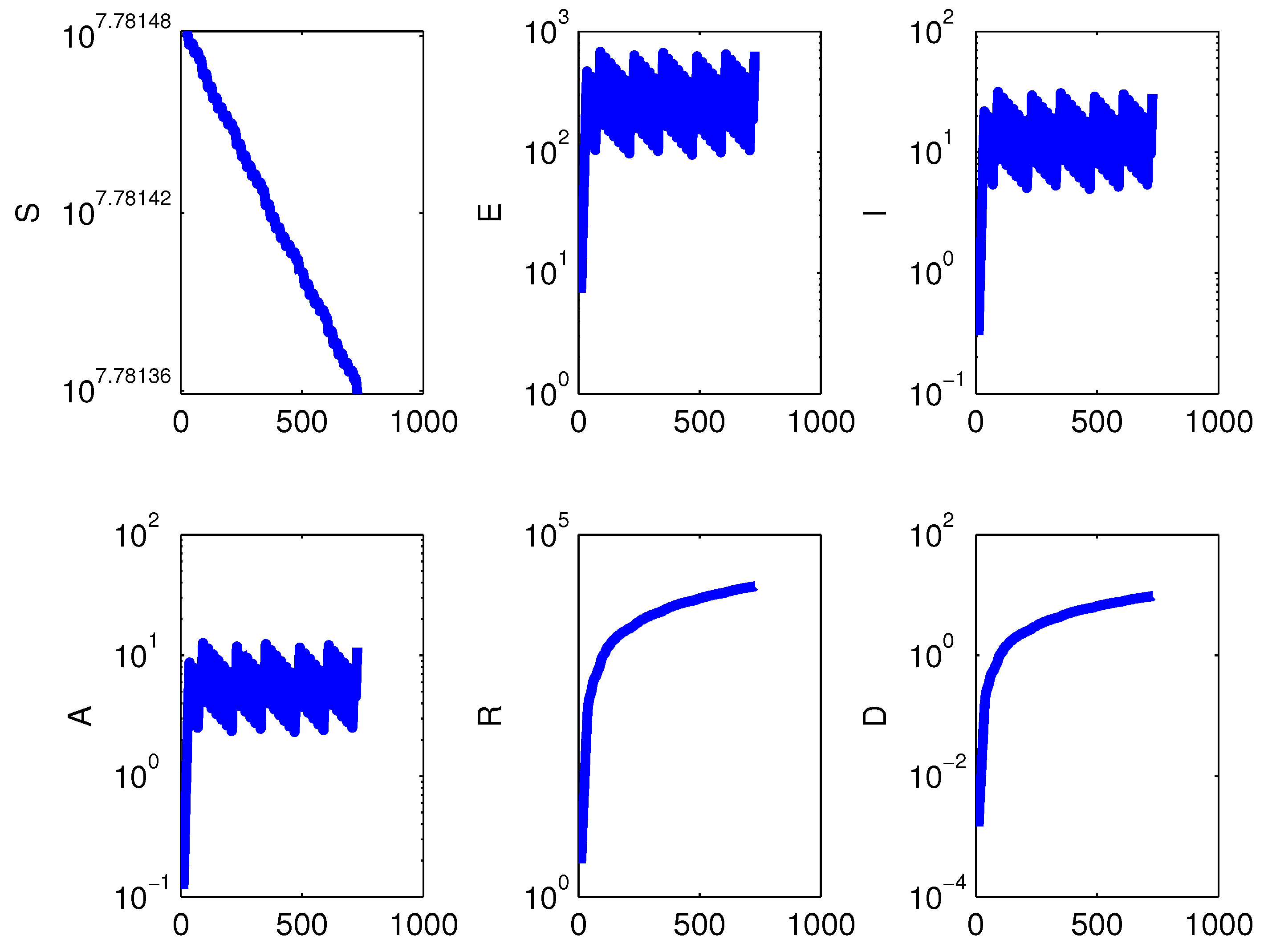
Using a semilogarithmic scale for the vertical axis, we show the results of starting the restrictions at time , using and lifting them at time , returning to one month later, over a one year timespan for the model with demographics (1). Left to right and top to bottom, the subpopulations are: S, E, I, A, R and D, the disease-related deceased class.
Figure 1.
Using a semilogarithmic scale for the vertical axis, we show the results of starting the restrictions at time , using and lifting them at time , returning to one month later, over a one year timespan for the model with demographics (1). Left to right and top to bottom, the subpopulations are: S, E, I, A, R and D, the disease-related deceased class.

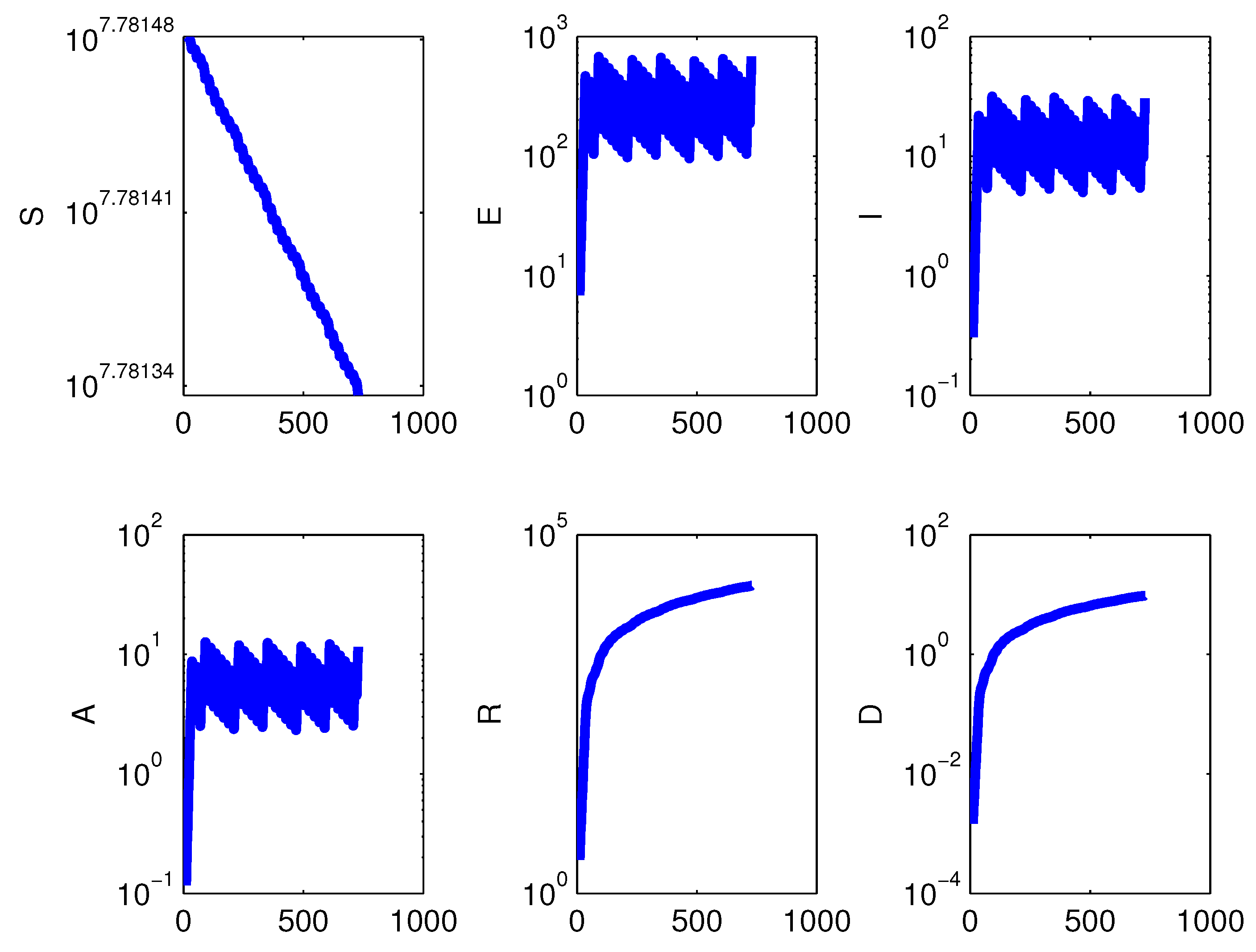
Figure 2.
Using a semilogarithmic scale for the vertical axis, we show the results of starting the restrictions at time , using and lifting them at time , returning to one month later, over a one year timespan for the model with demographics (1). Left to right and top to bottom, the subpopulations are: S, E, I, A, R and D, the disease-related deceased class.

Figure 3.
Using a semilogarithmic scale for the vertical axis, we show the results of starting the restrictions at time , using and lifting them at time , returning to three months later, over a one year timespan for the model with demographics (1). Left to right and top to bottom, the subpopulations are: S, E, I, A, R and D, the disease-related deceased class.

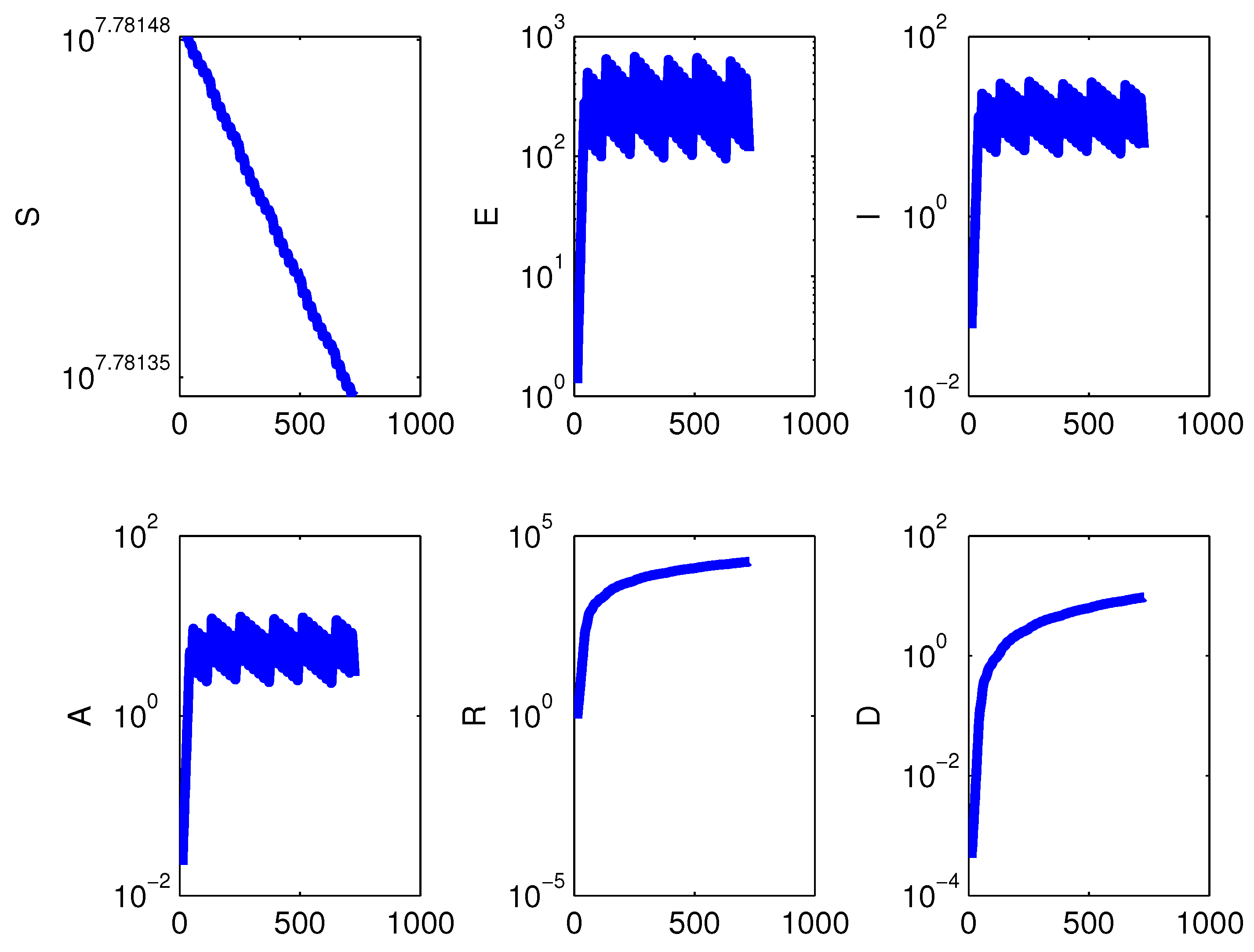
Figure 4.
Using a semilogarithmic scale for the vertical axis, we show the results of starting the restrictions at time , using and lifting them at time , returning to three months later, over a one year timespan for the model with demographics (1). Left to right and top to bottom, the subpopulations are: S, E, I, A, R and D, the disease-related deceased class.

Figure 5.
Using a semilogarithmic scale for the vertical axis, we show the results of absolute isolation, starting at time setting and lifting it at time , returning to one month later, over a one year timespan for the model with demographics (1). Left to right and top to bottom, the subpopulations are: S, E, I, A, R and D, the disease-related deceased class.

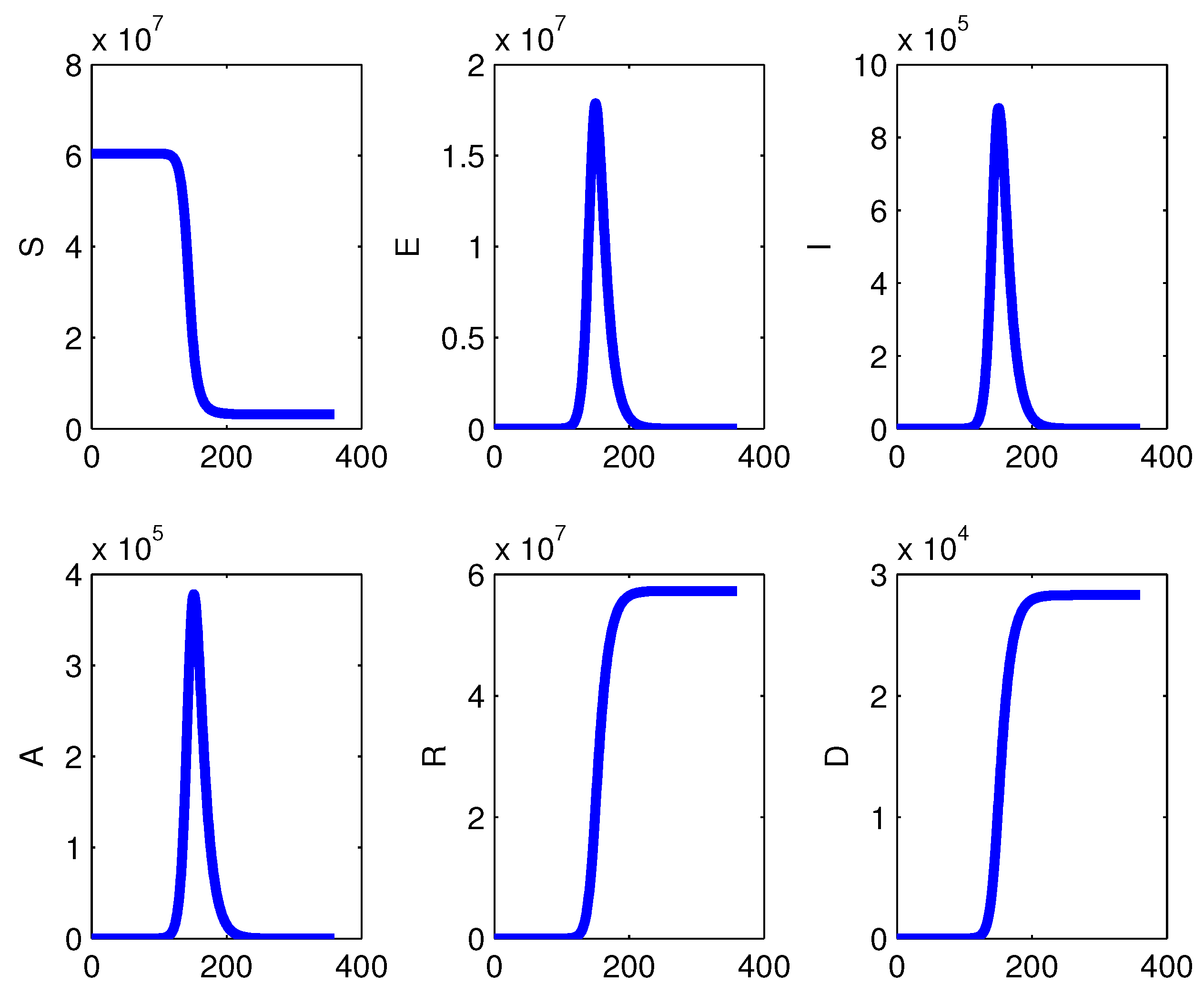
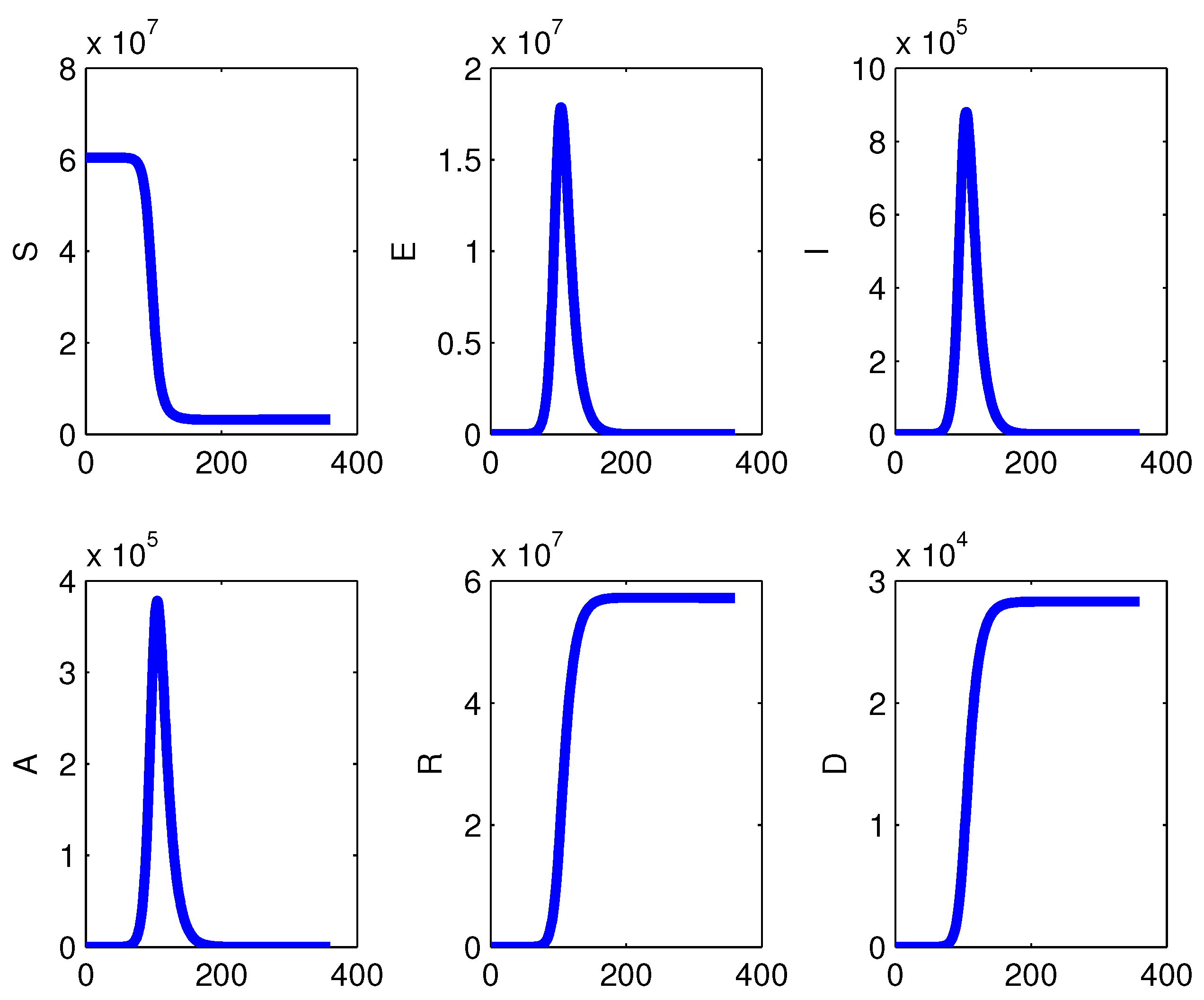
Figure 6.
The epidemic’s effect on the population in the absence of measures for , on a semilogarithmic scale, over a period of one year. Left to right and top to bottom: S, E, I, A, R and D, the disease-related deceased class.
Figure 6.
The epidemic’s effect on the population in the absence of measures for , on a semilogarithmic scale, over a period of one year. Left to right and top to bottom: S, E, I, A, R and D, the disease-related deceased class.

Figure 7.
On a semilogarithmic scale, the total populations with the lock-down policy, implemented from time 1 up to time 30, with the milder reduced contact rate , after which resumes. The simulation runs over a one year timespan for the simplified model (1). Left to right and top to bottom, the subpopulations are: S, E, I, A, R and D, the disease-related deceased class.

Figure 8.
Using a semilogarithmic scale for the vertical axis, we show the results of starting the restrictions at time , setting and lifting them at time , returning to one month later, over a one year timespan for the simplified model with no demographics (1) where we take , . Left to right and top to bottom, the subpopulations are: S, E, I, A, R and D, the disease-related deceased class.

Figure 9.
Using a semilogarithmic scale for the vertical axis, we show the results of starting the restrictions at time , setting and lifting them at time , returning to one months later, over a one year timespan for the simplified model with no demographics (1) where we take , . Left to right and top to bottom, the subpopulations are: S, E, I, A, R and D, the disease-related deceased class.

Figure 10.
Using a semilogarithmic scale for the vertical axis, we show the results of absolute isolation, starting at time , setting and lifting it at time , returning to three months later, over a one year timespan for the model with no demographics (1) where . Left to right and top to bottom, the subpopulations are: S, E, I, A, R and D, the disease-related deceased class.

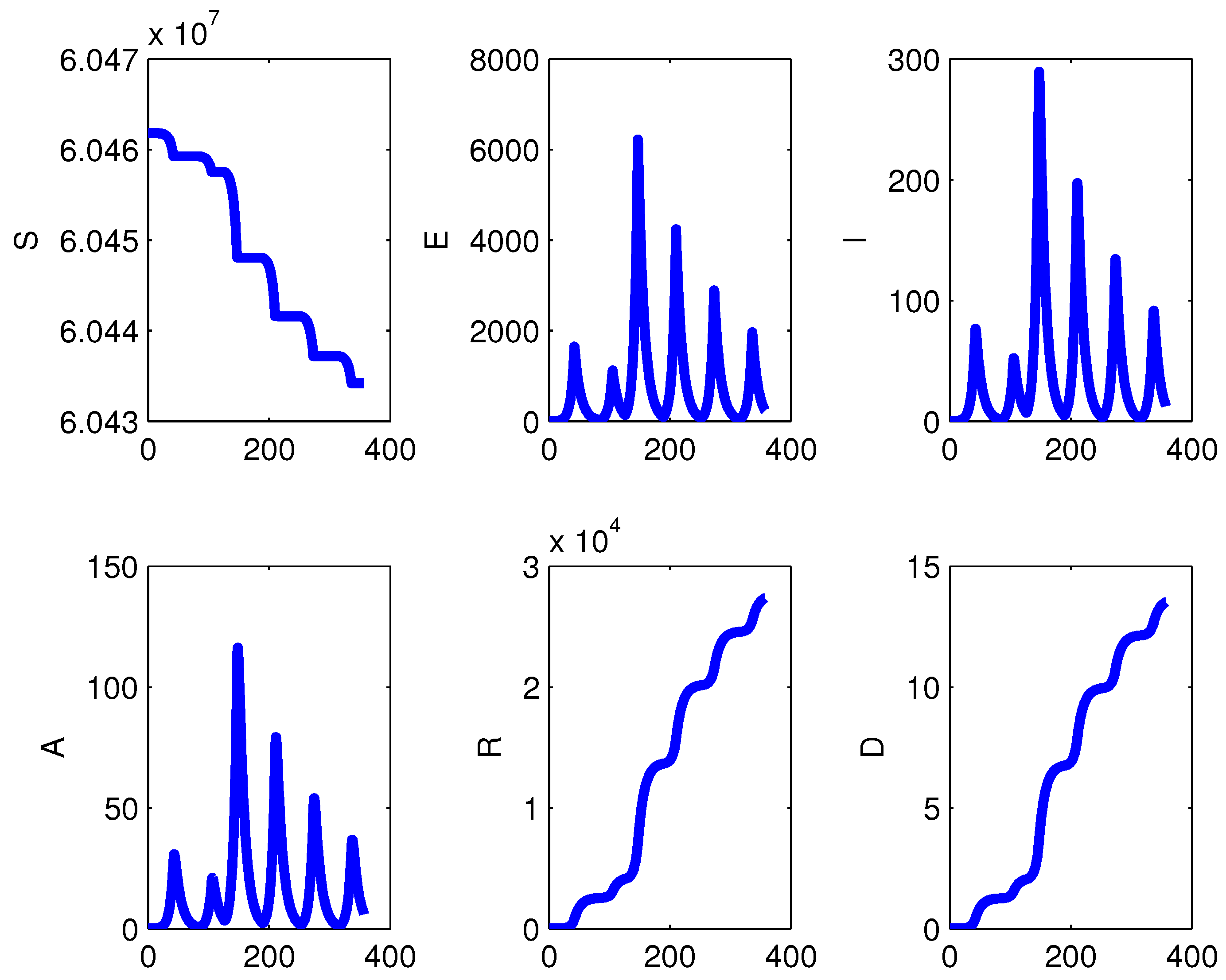
Figure 11.
The total populations with the lock-down policy, implemented from time 120 up to time 210, with the reduced contact rate , after which resumes. The simulation runs over a one year timespan for the model (1). Left to right and top to bottom, the subpopulations are: S, E, I, A, R and D, the disease-related deceased class.

Figure 12.
The total populations with the lock-down policy, implemented from time 90 up to time 120, with the total isolation policy , after which resumes. The simulation runs over a one year timespan for the simplified model (1) with no demographics, . Left to right and top to bottom, the subpopulations are: S, E, I, A, R and D, the disease-related deceased class.

Figure 13.
The semilogarithmic plot of the epidemic’s spread with the lock-down policy, implemented from time 90 up to time 180, with the reduced contact rate , after which resumes. The simulation runs over a one year timespan for the model (1) with demographics. Left to right and top to bottom, the subpopulations are: S, E, I, A, R and D, the disease-related deceased class.

Figure 14.
Using a semilogarithmic scale for the vertical axis, we show the results of the intermittent lock-down policy. Here the population is checked every week, starting after a week. If the number of infected is above a small threshold (here taken to be 10) the reduced contact rate is resumed for a week. The simulation runs over two years timespan for the model with demographics (1). Left to right and top to bottom, the subpopulations are: S, E, I, A, R and D, the disease-related deceased class.

Figure 15.
Using a semilogarithmic scale for the vertical axis, we show the results of the intermittent lock-down policy. Here the population is checked every week, starting after a week. If the number of infected is above a small threshold (here taken to be 10) the reduced contact rate is resumed for a week. The simulation runs over two years timespan for the simplified model with no demographics (1) where we take , . Left to right and top to bottom, the subpopulations are: S, E, I, A, R and D, the disease-related deceased class.

Figure 16.
Using a semilogarithmic scale for the vertical axis, we show the results of the intermittent lock-down policy, implemented from time 1. Here the population is checked every week. If the number of infected is above a small threshold (here taken to be 10) the reduced contact rate is resumed for a week. The simulation runs over two years timespan for the simplified model with no demographics (1) where we take , . Left to right and top to bottom, the subpopulations are: S, E, I, A, R and D, the disease-related deceased class.

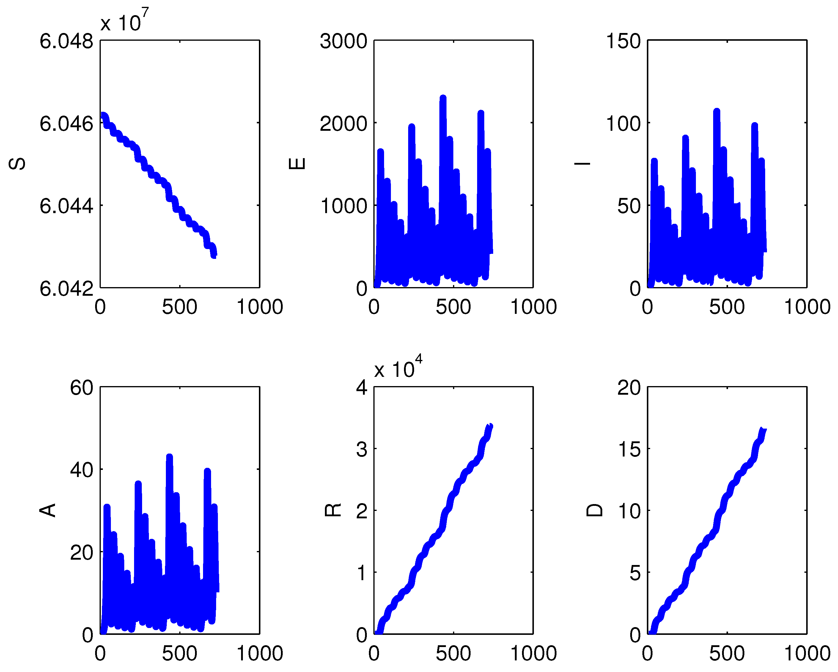
Figure 17.
The total populations with the intermittent lock-down policy, implemented from time 1. Here the population is checked every week. If the number of infected is above a small threshold (here taken to be 10) the reduced contact rate is resumed for a week. The simulation runs over two years timespan for the simplified model with no demographics (1) where we take , . Left to right and top to bottom, the subpopulations are: S, E, I, A, R and D, the disease-related deceased class.

Figure 18.
The total populations with the lock-down policy, implemented from time 1 up to time 30, with the reduced contact rate , after which resumes. The simulation runs over a one year timespan for the simplified model with no demographics (1) where we take , . Left to right and top to bottom, the subpopulations are: S, E, I, A, R and D, the disease-related deceased class.

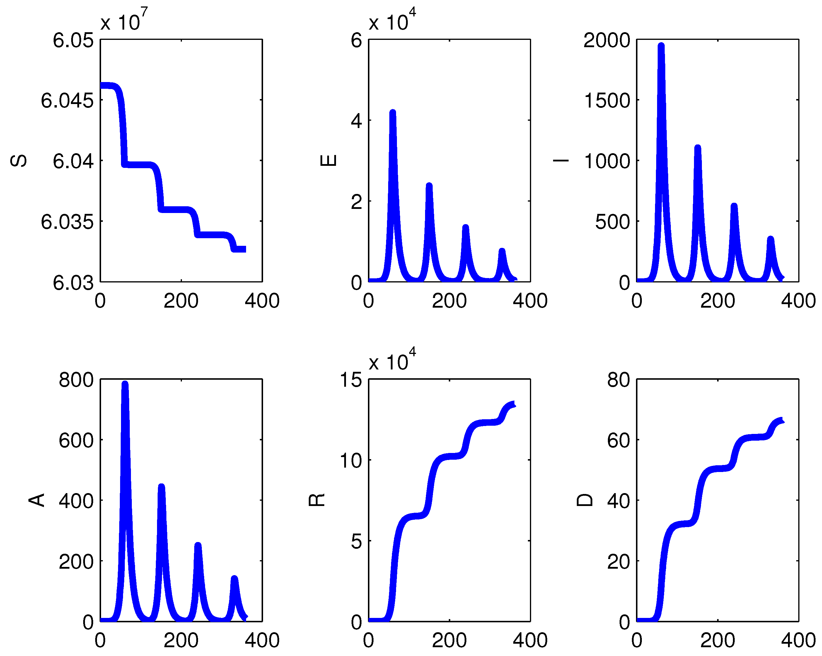
Figure 19.
The population values with the lock-down policy, implemented after the first week with the reduced contact rate , after which resumes. The check for possible repeated implementation is implemented every week afterwards. The simulation runs over a two years timespan for the model (1) with no demographics, i.e., . Left to right and top to bottom, the subpopulations are: S, E, I, A, R and D, the disease-related deceased class.

Figure 20.
The population values with the lock-down policy, implemented after the first two weeks with the reduced contact rate , after which resumes. The check for possible repeated implementation is implemented every two weeks afterwards. The simulation runs over a two year timespan for the model (1) with no demographics, i.e., . Left to right and top to bottom, the subpopulations are: S, E, I, A, R and D, the disease-related deceased class.

Figure 21.
The population values with the lock-down policy, implemented after the first thee weeks with the reduced contact rate , after which resumes. The check for possible repeated implementation is implemented every three weeks afterwards. The simulation runs over a two year timespan for the model (1) with no demographics, i.e., . Left to right and top to bottom, the subpopulations are: S, E, I, A, R and D, the disease-related deceased class.

Figure 22.
The population values with the lock-down policy, implemented after the first month with the reduced contact rate , after which resumes. The check for possible repeated implementation is implemented every month afterwards. The simulation runs over a two year timespan for the model (1) with no demographics, i.e., . Left to right and top to bottom, the subpopulations are: S, E, I, A, R and D, the disease-related deceased class.

Figure 23.
The basic interactions among the compartments.

Figure 24.
The susceptible population behavior over a year, without disease. It does not vary much as the vertical scale is rather small, the range of variation being around 3000, over a population of .
Figure 24.
The susceptible population behavior over a year, without disease. It does not vary much as the vertical scale is rather small, the range of variation being around 3000, over a population of .

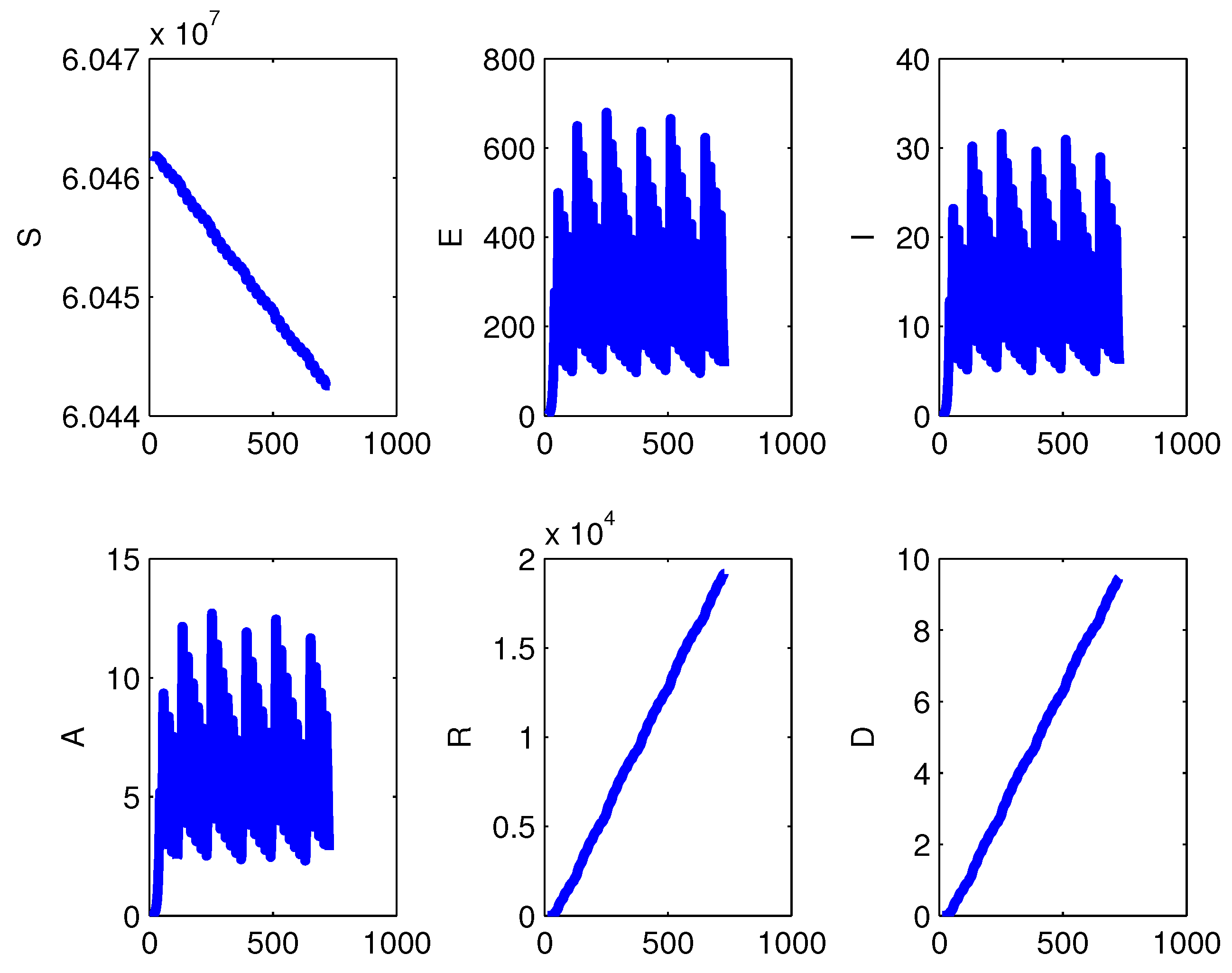
Figure 25.
The epidemic’s effect on the population in the absence of measures for , over a period of one year. Left to right and top to bottom, the total population sizes: S, E, I, A, R and D, the disease-related deceased class.
Figure 25.
The epidemic’s effect on the population in the absence of measures for , over a period of one year. Left to right and top to bottom, the total population sizes: S, E, I, A, R and D, the disease-related deceased class.


Table 1.
Equilibria of the model (1) and their feasibility conditions.
Table 1.
Equilibria of the model (1) and their feasibility conditions.
| Equilibrium | Populations | Feasibility |
|---|---|---|
| – | ||
| (resp. ) | ||
| and | ||
| (resp. ) | ||
| or | ||
Table 2.
Stability conditions of the equilibria of the model (1).
Table 2.
Stability conditions of the equilibria of the model (1).
| Point | Coefficients | Stability |
|---|---|---|
| (resp. ) | ||
| , | ||
| (resp. ) | ||
| and | ||
| , | ||
| (resp. ) | ||
| or | ||
Table 3.
Parameters values.
| Parameter | Value | Parameter | Value |
|---|---|---|---|
| 500 | |||
| k | [0:005; 0:2] | ||
| 0 |
Table 4.
Model parameters and their meaning.
| susceptibles recruitment rate | |
| natural mortality | |
| disease transmission rate | |
| k | transmissibility ratio between asymptomatics and symptomatics |
| disease-related mortality for infected | |
| disease-related mortality for asymptomatics | |
| progression rate from exposed to symptomatic | |
| progression rate from exposed to asymptomatic | |
| fraction of exposed that turn asymptomatic | |
| progression rate from asymptomatic to symptomatic | |
| recovery rate from symptomatic infection | |
| recovery rate from asymptomatic infection |
© 2020 by the authors. Licensee MDPI, Basel, Switzerland. This article is an open access article distributed under the terms and conditions of the Creative Commons Attribution (CC BY) license (http://creativecommons.org/licenses/by/4.0/).
Share and Cite
MDPI and ACS Style
Belgaid, Y.; Helal, M.; Venturino, E. Analysis of a Model for Coronavirus Spread. Mathematics 2020, 8, 820. https://doi.org/10.3390/math8050820
AMA Style
Belgaid Y, Helal M, Venturino E. Analysis of a Model for Coronavirus Spread. Mathematics. 2020; 8(5):820. https://doi.org/10.3390/math8050820
Chicago/Turabian StyleBelgaid, Youcef, Mohamed Helal, and Ezio Venturino. 2020. "Analysis of a Model for Coronavirus Spread" Mathematics 8, no. 5: 820. https://doi.org/10.3390/math8050820
Note that from the first issue of 2016, this journal uses article numbers instead of page numbers. See further details here.