Analyzing COVID-19 Impacts on Vehicle Travels and Daily Nitrogen Dioxide (NO₂) Levels among Florida Counties

Abstract

The COVID-19 outbreak and ensuing social distancing behaviors resulted in substantial reduction on traffic, making this a unique experiment on observing the air quality. Such an experiment is also supplemental to the smart city concept as it can help to identify whether there is a delay on air quality improvement during or after a sharp decline on traffic and to determine what, if any, factors are contributing to that time lag. As such, this study investigates the immediate impacts of COVID-19 causing abrupt declines on traffic and NO₂ concentration in all Florida Counties through March 2020. Daily tropospheric NO₂ concentrations were extracted from the Sentinel-5 Precursor satellite and vehicle mile traveled (VMT) estimates were acquired from cell phone mobility records. It is observed that overall impacts of the COVID-19 response in Florida have started in the first half of the March 2020, two weeks earlier than the official stay-at-home orders, and resulted in 54.07% and 59.68% decrease by the end of the month on NO₂ and VMT, respectively. Further, a cross-correlation based dependency analysis was conducted to analyze the similarities and associated time lag between 7-day moving averages of VMT and NO₂ concentrations of the 67 counties. Although such reduction is unprecedented for both data sets, results indicate a strong correlation and this correlation increases with the identification of a time lag between VMT and NO₂ concentration. Majority of the counties have no time lag between VMT and NO₂ concentration; however, a cluster of South Florida counties presents earlier decrease on NO₂ concentration compare to VMT, which indicates that the air quality improvements in those counties are not traffic related. Investigation on the socioeconomic factors indicates that population density and income level have no significant impact on the time lag between traffic and air quality improvements in light of COVID-19.

1. Introduction

The coronavirus disease 2019 (COVID-19) and ensuing social distancing behaviors have caused unprecedented changes in every aspect of modern life. Beyond the devastating impacts on human’s health, daily life has changed tremendously to stop the spread of the novel coronavirus (SARS-CoV-2). In late 2019, the first cases of the coronavirus disease 2019 (COVID-19) were reported in Wuhan, China. It then quickly swept through many countries and was declared as a global pandemic in March 2020. Despite the devastating impacts on public health, modern life has completely changed to stop the spread of the virus by limiting human activities.

As of 31 July, more than 660 thousand people have died and more than 17 million people have been exposed to this new virus around the world [1]. Meanwhile, most global stock markets reported severe contractions in March 2020 [2], substantial increases were observed on unemployment, school campuses were closed, and majority of remaining work activities have been performed remotely. To combat with this virus and analyze the impacts on various fields, the scientific community all over the world have come together in a truly unprecedented way.

In regards to the influence on the transportation and mobility, all the published literature states that overall mobility has dropped significantly due to the spread of the virus [3,4]. The success of a lockdown policy in China led most of the countries to apply similar countermeasures that mainly restricted mobility. An analysis carried out by INRIX [5] found a 60% reduction in commuting travels and 26% improvement on travel times in the City of Seattle using data from early March. In addition, commercial data providers such as Unacast Inc. [6] or StreetLight Data Inc. [7] provided free access to their daily county level vehicle miles traveled (VMT) data sets. The global mobility reports provided by Google [8] revealed a worldwide reduction in the number of trips. As a result of these unprecedented changes on traffic demand, significant decreases were observed on traffic accidents, public transportation use, and air pollution [9,10].

It has been known that air pollution is linked to different types of cardiovascular and respiratory diseases, which leads to millions of premature deaths across the world every year. Indeed, a study estimated a monthly reduction of 360 premature deaths in the U.S. due to the air quality improvements as a result of the decrease on traffic and electric use during the outbreak [3]. However, long term estimations on the immediate impact of COVID-19 may not be an accurate assumption. Short-run impact on air quality can easily be outweighed in long-run effects of a decreasing clean energy innovation [10]. Regardless, analyzing the relationship between traffic and air quality especially during these unprecedented times can help the cities with severe air pollution determine proper traffic restriction policies. For example, a study from India [11] suggested to continue with selected traffic restricted zones after observing a significant decrease on air pollution during the COVID-19 conditions.

Short-term effects of COVID-19 on air quality have also been widely studied with remote sensing technology. NASA has partnered with the European Space Agency (ESA) to analyze how the shutdowns in response to the pandemic are changing the environment, especially the atmosphere [12]. Preliminary results indicates that COVID-related impacts were harder to see on sulfur dioxide (SO₂) while significant reductions were observed on nitrogen dioxide (NO₂) density over China [13] and over the United States [14]. Similarly, NOAA’s Joint Polar Satellite System indicates an evident drop in NO₂ levels and particulate matter (PM) between March 2019 and 2020 [15]. Further analyses are required to measure the particular impact of traffic reduction on these unusual air quality improvements. However, remotely sensed air pollution sources specifically show the decreased NO₂ concentrations as an impact of decreased human activity due to COVID-19.

Nitrogen dioxide (NO₂) takes a place among the highly reactive gases with other Nitrogen oxides (NO_x). Natural NO₂ emission sources such as biomass, nitrates of microbial reactions or atmospheric lightening process, have a very small contribution compare to the anthropogenic NO₂ emission sources, which mainly include burning of fuel, industrial production, and agricultural burning [16]. NO₂ reacts with other chemicals in the air to form particulate matter and ozone, which are harmful to the respiratory system when inhaled. Additionally, NO₂ interacts with water, oxygen, and other chemicals in the atmosphere to form acid rain, which harms sensitive ecosystems such as lakes and forests. Therefore, NO₂ is considered as one of the six criteria pollutants in National Ambient Air Quality Standards (NAAQS), which were established by U.S. Environmental Protection Agency (USEPA) through the Clean Air Act [17,18]. NO₂ is continuously monitored across the U.S. so that those areas where the air quality does not meet the national standards can be identified and state implementation plans (SIPs) can be developed to combat NO₂ pollution [19].

Given the preliminary results from space, transportation, and environmental agencies, recent studies analyzing the impact of COVID-19 on the air quality (Table 1) also indicate a decrease on NO₂ levels due to COVID-19. Although other air pollutants vary based on the nature of implementation of the lockdown or additional pollution sources such as coal, a decrease in NO₂ has been seen in all studies. However, all these studies used surface-based sensors to acquire pollutant measurements. Although current regulatory compliance on air quality is performed mostly by surface sensors, the advancements in remote sensing methods and the availability of satellite data create new opportunities to use space level technologies to monitor every part of atmosphere rather than point observations on surface. The rapid development of the remote sensing monitoring methods of atmospheric satellite have gradually become critical technical means of global atmospheric monitoring [16]. Thus, there is a need to evaluate the results with the satellite-retrieved air pollution measurements.

As such, the objective of this study is twofold: first, we evaluated the relationship between traffic and NO₂ concentrations in the wake of COVID 19 to determine whether there was a delay in air quality improvement during or after a sharp decline in traffic. The second aim is to determine, which, if any, factors affect this time lag and the overall correlation between traffic and NO₂ concentrations. County level daily NO₂ levels are extracted from Sentinel-5P satellite of ESA, expected to change the way the air quality is monitored today [20] and vehicle mile traveled (VMT) estimates are acquired from cell phone mobility records. Population density, median income, and the percentage of the households with no vehicle are also obtained for each county from the U.S. Census’s 2018 American Community Surveys [21]. Cross-correlation based dependency analysis is conducted with the Pearson’s r statistic to analyze the similarities and associated time lag between 7-day moving averages of VMT and NO₂ concentration of 67 Florida counties. Such evaluation of the time-lag between the vehicle miles travelled (VMT) and NO₂ can be used as a time-offset for smarter cities in order to find ways to link air pollution and traffic. The novelty of this study as follows:

• Using satellite technology to evaluate the NO₂ concentrations and traffic as continuous time signals in the wake of COVID-19,
• Providing an in-depth county level dependency analysis to determine the time lag between traffic reduction and air quality improvement,
• Investigating the impact of socioeconomic factors on the traffic–air quality relationship.

Table 1. Example studies of COVID-19 impacts on air quality and their findings.

Study	Location	Pollution Data	Traffic Data	Analysis Periods	Key Findings
Berman and Ebisu [22]	Continental US	Surface Sensors from OpenAQ [23]	N/A	8 January–12 March 13 March–21 April 2017–2019	Average 25.5% NO2 decrease Rural area NO2 decrease is smaller (16.5%) Average 4.45% decrease on PM2.5 States with late or no stay-at-home order have increase (3.51%) on PM2.5 but 11.26% decrease on early stay-at-home order states
Bekbulat et al. [24]	Continental US	Surface sensors from USEPA [25]	N/A	After official stay-at-home order in each state 2010–2019	Nationwide analysis for PM2.5 and O3 and 3 cities for NO2 30% decrease on NO2 but no significant decrease on PM2.5 and O3 PM2.5 and O3 medians are decreasing 2 weeks before the stay-at-home orders but after it converges back with national averages. For NO2 in NYC, LA, and Seattle decrease starts at 9th week before shutdown.
Jia [26]	Memphis, TN	Local stations From USEPA [25]	StreetLight [7]	Prior Month (25 February–24 March) Lockdown (25 March–4 May) Baseline 2017–2019 April	57% reduction on traffic, no air-monitoring station near roadway. No significant reduction on PM2.5, O3 during the lockdown compare to nor before lockdown neither same days last years NO2 measured from only 1 station. Small reduction observed on the mean compare to prior month and 12% increase compare to the baseline periods Estimation models indicate only wind speed is significant on estimating the NO2 (Not lockdown, temperature, or precipitation). Traffic is not included
Collivignarelli et al. [27]	Milan, Italy	Surface stations from the Local Agency	N/A	Control (7–20 February) Partial lockdown (9–22 March) Total lockdown (23 March–5 April)	Total lockdown caused 61% and 74.5% reduction in the city center on NO2 and NOx, respectively. 47.4% and 48% decrease on PM10 and PM2.5 Substantial increase on O3 due to minor NO2 concentration Study periods are separated based on the temperature, humidity, wind, precipitation, and solar irradiance.
Mahato et al. [28]	Delhi, India	Surface Stations from the Local Agency	N/A	Pre Lockdown After Lockdown	+50% decrease on PM10 and PM2.5 52.68% and 30.35% decrease on NO2 and CO respectively
Baldasano [29]	Barcelona and Madrid, Spain	Surface sensors from the Local Agency	Google [8]	March 2020 March 2018/19	62% and 50% NO2 decrease in Madrid and Barcelona, respectively 75% reduction in traffic NO2 reduction in urban traffic area higher than urban and rural areas
Kerimray et al. [30]	Almaty, Kazakhstan	Surface stations from the Local Agency	N/A	2–18 March 19 March–14 April	35% NO2 and 49% CO reduction due to the seasonal changes and traffic reduction. Increase on SO2 (7%) and O3 (15%). Seasonal reduction due to the reduction in coal use is more effective than traffic reduction. 21% reduction on PM2.5 compare to last year with high variation.

Table 1. Example studies of COVID-19 impacts on air quality and their findings.

Study	Location	Pollution Data	Traffic Data	Analysis Periods	Key Findings
Berman and Ebisu [22]	Continental US	Surface Sensors from OpenAQ [23]	N/A	8 January–12 March 13 March–21 April 2017–2019	Average 25.5% NO2 decrease Rural area NO2 decrease is smaller (16.5%) Average 4.45% decrease on PM2.5 States with late or no stay-at-home order have increase (3.51%) on PM2.5 but 11.26% decrease on early stay-at-home order states
Bekbulat et al. [24]	Continental US	Surface sensors from USEPA [25]	N/A	After official stay-at-home order in each state 2010–2019	Nationwide analysis for PM2.5 and O3 and 3 cities for NO2 30% decrease on NO2 but no significant decrease on PM2.5 and O3 PM2.5 and O3 medians are decreasing 2 weeks before the stay-at-home orders but after it converges back with national averages. For NO2 in NYC, LA, and Seattle decrease starts at 9th week before shutdown.
Jia [26]	Memphis, TN	Local stations From USEPA [25]	StreetLight [7]	Prior Month (25 February–24 March) Lockdown (25 March–4 May) Baseline 2017–2019 April	57% reduction on traffic, no air-monitoring station near roadway. No significant reduction on PM2.5, O3 during the lockdown compare to nor before lockdown neither same days last years NO2 measured from only 1 station. Small reduction observed on the mean compare to prior month and 12% increase compare to the baseline periods Estimation models indicate only wind speed is significant on estimating the NO2 (Not lockdown, temperature, or precipitation). Traffic is not included
Collivignarelli et al. [27]	Milan, Italy	Surface stations from the Local Agency	N/A	Control (7–20 February) Partial lockdown (9–22 March) Total lockdown (23 March–5 April)	Total lockdown caused 61% and 74.5% reduction in the city center on NO2 and NOx, respectively. 47.4% and 48% decrease on PM10 and PM2.5 Substantial increase on O3 due to minor NO2 concentration Study periods are separated based on the temperature, humidity, wind, precipitation, and solar irradiance.
Mahato et al. [28]	Delhi, India	Surface Stations from the Local Agency	N/A	Pre Lockdown After Lockdown	+50% decrease on PM10 and PM2.5 52.68% and 30.35% decrease on NO2 and CO respectively
Baldasano [29]	Barcelona and Madrid, Spain	Surface sensors from the Local Agency	Google [8]	March 2020 March 2018/19	62% and 50% NO2 decrease in Madrid and Barcelona, respectively 75% reduction in traffic NO2 reduction in urban traffic area higher than urban and rural areas
Kerimray et al. [30]	Almaty, Kazakhstan	Surface stations from the Local Agency	N/A	2–18 March 19 March–14 April	35% NO2 and 49% CO reduction due to the seasonal changes and traffic reduction. Increase on SO2 (7%) and O3 (15%). Seasonal reduction due to the reduction in coal use is more effective than traffic reduction. 21% reduction on PM2.5 compare to last year with high variation.

2. Materials and Methods

2.1. Study Area

The state of Florida was selected as the test bed in this study. With a population of over 21 million, Florida is the third-most populous of the 50 states. Florida includes 67 counties where the populations of these counties range from 2 million to 8000. Figure 1 indicates the population density of each county where those counties that host cities of Miami, Tampa, Orlando, and Jacksonville appear to be the most populated ones. In addition, according to the Centers for Disease Control and Prevention (CDC), the older population (65+) and those with serious medical conditions such as lung disease, diabetes, liver disease, etc., are at a higher risk of COVID-19 infection [31]. Hence, this becomes a serious issue in Florida since more than 20% of the total population in the state are 65 years and older [21]. Therefore, the impact of COVID-19 on these populations becomes all the more confounding in light of their potential health and other safety concerns.

2.2. Data Description

Generally, NO₂ pollutant measurement is performed in two different ways: ground-based [23,25,26,32] and remote sensing-based methods [16,20,33]. In ground-based methods, NO₂ is measured in air quality monitoring stations where NO₂ values are recorded several times a day using a set of sensors specifically designed to perform this task. While surface measurements serve as the tools for regulatory compliance, these measurements are limited to a few stations scattered over an area. In the remote sensing approach, on the other hand, NO₂ and other atmospheric trace gases are identified and measured by their signature spectral lines left in the reflected sun light on to the spectrometers. In the recent decades, advances in technology and reduced costs of building and launching satellites have made remote sensing a popular method for air quality monitoring; however, this method still lacks the required resolution to measure NO₂ and other atmospheric trace gases at the roadway level. A recent example of remotely monitoring NO₂ and other atmospheric trace gases is the Sentinel-5P, which has reached the city level resolution with 5 km × 3.5 km (3.1 mi × 2.2 mi) pixel size (improved from 7 km × 3.5 km (4.3 mi × 2.2 mi) in August 2019).

The Copernicus Sentinel-5 Precursor, known as Sentinel-5P, is a satellite in the series of Copernicus Sentinel satellites dedicated to atmospheric monitoring. This is a joint program between the European Space Agency (ESA), the European Commission, the Netherlands Space Office, industry, data users, and scientists. Copernicus Sentinel-5P was successfully launched on 13 October 2017 with a planned mission of seven years [34]. It aims to provide routine observations of atmospheric trace gases and aerosols. The sensor on board, tropospheric monitoring instrument (TROPOMI) is a spectral based device that uses the UV–Visible, NIR, and SWIR bands to measure key atmospheric components such as ozone (O₃), sulphur dioxide (SO₂), carbon monoxide (CO), methane (CH4), and formaldehyde (HCHO) additional to NO₂ [33]. Technology in TROPOMI has benefited from its predecessor instruments the ozone monitoring instrument (OMI) and scanning imaging absorption spectrometer for atmospheric cartography (SCIAMACHY) [33].

For the purposes of this study, 34 files were downloaded from Sentinel-5P data hub [35]. For each day, there were several files in the data hub repository; however, an attempt was made to only download those files that had the total coverage over the State of Florida on a given date. There were 3 days (i.e., March 3, 8, and 19) on which there was no single file with the total coverage of Florida. Thus, three extra files were downloaded for these days. Next, data preparation was conducted with Python programming language. Careful attention was paid to ensure that the quality of data was not compromised. For this purpose, two different filters were applied to the input datasets for masking out faulty pixel values. The first filter masked out all pixels with NO₂ values below zero and the second filter masked out all pixels with quality-flag below 0.75, which is the recommended value in the user manual of the data set [36]. The result was a set of pixels with NO₂ constriction values above zero and quality-flag value equal to or above 0.75. In the next step, using a county-level polygon geojson file (with a resolution of 20 m), each county was carefully extracted along with its associated NO₂ pixel values within the county. At this point, each county had a set of masked out and useful pixels. To estimate the average NO₂ over each county on a given day, we only used NO₂ values of the useful pixels. Additionally, we defined a parameter, called the coverage ratio, which indicates the fraction of useful pixels over a county to the total number of pixels in that county on a given day. The final product of this procedure was a list of counties with a mean value of NO₂ and coverage ratio over that county for each day of the March 2020. This process is summarized in Figure 2 with a flowchart. Additionally, NO₂ concentration measurements of 2 example dates from March are illustrated in Figure 3. Note that the immediate impact of COVID is visible especially on the east side where Hillsborough and Pinellas counties are located. Since NO₂ concentration fluctuates between weekdays and weekends [20], 7-day moving averages were calculated for each county. This also helped interpolating the missing data due to the quality masking.

The daily vehicle miles traveled (VMT) estimates for each county were extracted from StreetLight Data Inc. This commercial mobility data provider created a pro bono COVID-19 data set to help researchers and raise public awareness on social distancing. The data set includes daily VMTs of the U.S. counties beginning from 1 March. As a baseline, the average January 2020 VMTs are also provided for each county. StreetLight’s VMT estimates are based on the data collected from the smart phone apps providing location-based services and GPS trackers on commercial fleets [37]. In general, the daily VMT estimates were calculated by using the VMT of previous months as the baseline and multiplying the calculated mean trip length with the total number of trips. More details on their methodological and validation approach can be found in [38]. To avoid the fluctuation between weekdays and weekend VMTs, 7-day moving averages were calculated for the month of March 2020.

In addition, population density, median income and the percentage of the households with no vehicle data for each county were also obtained from the US Census’s 2018 American Community Survey [21].

2.3. Data Analysis Approach

Cross-correlation is a well-known measure of similarity of two series as a function of the displacement [39]. It measures the sliding dot product of two signals that turns a larger value when both signals are following a similar pattern and vice versa. Normalization of cross-correlation is a common approach to test the similarities of signals with different units (i.e., VMT and NO₂ concentration), which can be interpreted as time dependent Pearson correlation coefficient [40]. Mathematically, normalized cross correlation can be defined as:

$$\rho \left(\tau \right)=\frac{E\left[(X_t-{\mathsf{\mu }}_X\right)\left(Y_{t+\tau }-{\mathsf{\mu }}_Y\right)]}{{\sigma }_X{\sigma }_Y}$$

(1)

where the correlation between $X_t$ and $Y_t$ is calculated by sliding the $Y_t$ signal with $\tau$ time step- or so-called lag. $\rho \left(\tau \right)$ represents the correlation coefficient on the lag $\tau$ and takes a place in [−1, 1]. −1 indicates perfect anticorrelation, and 1 indicating perfect correlation between the tested variables.

In this study, maximum cross correlation, $\rho \left({\tau }^{\ast }\right)$ was calculated for 7-day moving averages of VMT and NO₂ concentration of each Florida county. ${\tau }^{\ast }$ could be interpreted as the time lag between VMT and NO₂ concentration through March 2020. If this value is negative, it indicates that the NO₂ decrease started after the VMT decrease, which shifts NO₂ to the left side on time providing a higher correlation. Additionally, $\rho \left(0\right)$ reveals the natural correlation coefficient between VMT and NO₂ concentration without any time sliding. Finally, a county with a positive ${\tau }^{\ast }$ value has observed the NO₂ decline earlier than the VMT decline and thus sliding its NO₂ concentration to the right side resulting in a higher correlation with VMT.

To understand what effects the time lag between VMT and NO₂, other data such as population density, median income, and the percentage of the households and the heavy vehicle percentage in the registered vehicles were investigated in each county.

3. Results

3.1. Short-Term Effects of COVID-19 in Daily Travel and NO₂ Emissions

Although a nation-wide lockdown has never been initiated in the U.S., social distancing behaviors such as teleworking and shifting to online teaching have led to a drastic decrease on overall mobility of the nation. StreetLight Data’s pro bono vehicle mile traveled (VMT) data [7] for the U.S. counties highlight this impact. Figure 4a indicates the 7-day moving average of VMT for all counties in the U.S. included in the dataset whereas Figure 4b depicts the 67 Florida Counties along with 7-day moving averages of tropospheric NO₂ concentrations during March 2020. Additionally, January 2020 VMT averages and a generalized timeline of COVID-19 impact/respond is highlighted in Figure 4. It can be observed that, in the second half of the analyzing period, traffic demand decreased approximately 60% in both FL and the entire U.S. Although it varies based on the local government responses, the abrupt decline starts on 13 March, Friday with the national emergency and global outbreak announcements. Additionally, most of the universities started their spring break on this date and shifted to online teaching until the end of the semester. In Florida, stay-at-home order was first mandated 2 weeks later, on 31 March for only three counties: Miami-Dade, Broward, and Palm Beach, then on 1 April for the entire state [41]. A study [3] analyzed the mobility differences between the early-policy states that put a stay-at-home policy in place by 28 March, and the states with no policy by the same date. Both Florida and the U.S. VMTs fall below the January average on 17th, which is similar to the late or no policy states found in that study [3].

As aforementioned, the NO₂ concentration over an area is strongly related with human activities. Therefore, it is not surprising that a parallel pattern was observed between 7-day moving averages of VMT and NO₂ concentration. To indicate the short-term effect of COVID-19, percentage decreases of VMT and NO₂ concentration were calculated based on their maximum and minimum values observed in March for each county:

$$\left[\left(max-\min \right)/max\right]\ast 100$$

(2)

Among 67 Florida Counties, an average of 54.07% and 59.68% decrease were observed for 7-day moving averages of NO₂ and VMT, respectively. The distributions of these percentage decreases are presented in Figure 5. Furthermore, the distributions for the dates in March when the maximum and minimum values were observed for 7-day moving averages of VMT and NO₂ concentrations in each county are presented in Figure 6. Results indicate that vehicle use in most of the counties started to decrease after the Friday, 13 March until the end of the month. This is more than 2 weeks before the official stay-at-home order was initiated in Florida on 1 April. This clearly indicates that social distancing behaviors have affected the traffic and air quality before the official policy enacted and this should be considered by further studies on the air quality impacts of COVID-19 to determine the study periods.

Despite the persistence on the days when the highest and lowest VMT values were observed in different counties, NO₂ concentration observations depicted more variation on the days when maximum and minimum values were observed. This can be attributed to different reasons including the weather characteristics of the county, the level of urbanization (i.e., urban or rural), main industry, and vehicle distribution, which may prevent the NO₂ particles to get concentrated or change the impact of the COVID at a particular county. The relationship between VMT and NO₂ concentration is visible on the 7-day average diagrams; however, a cross-correlation-based dependency analysis can investigate the time lag, if there is any.

3.2. Dependency Analysis on VMT and NO₂ Trends

Even with the abrupt decline, the immediate impact of COVID-19 in March 2020 indicates a similar behavior for both vehicle mile traveled (VMT) and nitrogen dioxide (NO₂) density in Florida. To investigate this similarity and influencing factors, a cross-correlation analysis was conducted by calculating the correlation coefficients with step size of 1-day displacement between 7-day moving averages of VMT and NO₂ concentration for each county. As mentioned in methodology section, the time lag is considered where the maximum correlation is calculated. A particular interest is to determine whether the socioeconomic factors such as population and income have an impact on the time lag between the VMT and NO₂.

Figure 7 depicts the positive, zero, and negative time lags (τ*) in each row for the counties with a high population density on the left column and a low population density on the right column. For Miami-Dade County, the decrease of NO₂ concentration started 5 days earlier than the decrease on VMT since the correlation increased from 0.65 to 0.80 by shifting the NO₂ concentration 5 days further. Miami-Dade County accommodates the highest number of population compared to other counties of Florida (19) and it has been hit the hardest by COVID-19. The county currently has approximately the 25% of all confirmed cases in the entire state. Although the first case was confirmed in Hillsborough County, the VMT and NO₂ concentration started to decrease later than Miami-Dade County. Note that the lowest correlation was observed for the counties where NO₂ concentration started to decrease after VMT. This may occur due the extra fluctuation on the NO₂ levels, which can be attributed to many reasons such as unfavorable weather, commercial, or industrial manufacturing.

To investigate the impact of economic status of the counties on the correlation between VMT and NO₂ concentration, counties with higher and lower median household income were compared in Figure 8. Although the economic status of the area had a significant impact on the overall NO₂ concentration, no significant impact was observed on the correlation between VMT and NO₂ from the median income similar to the one with the population density.

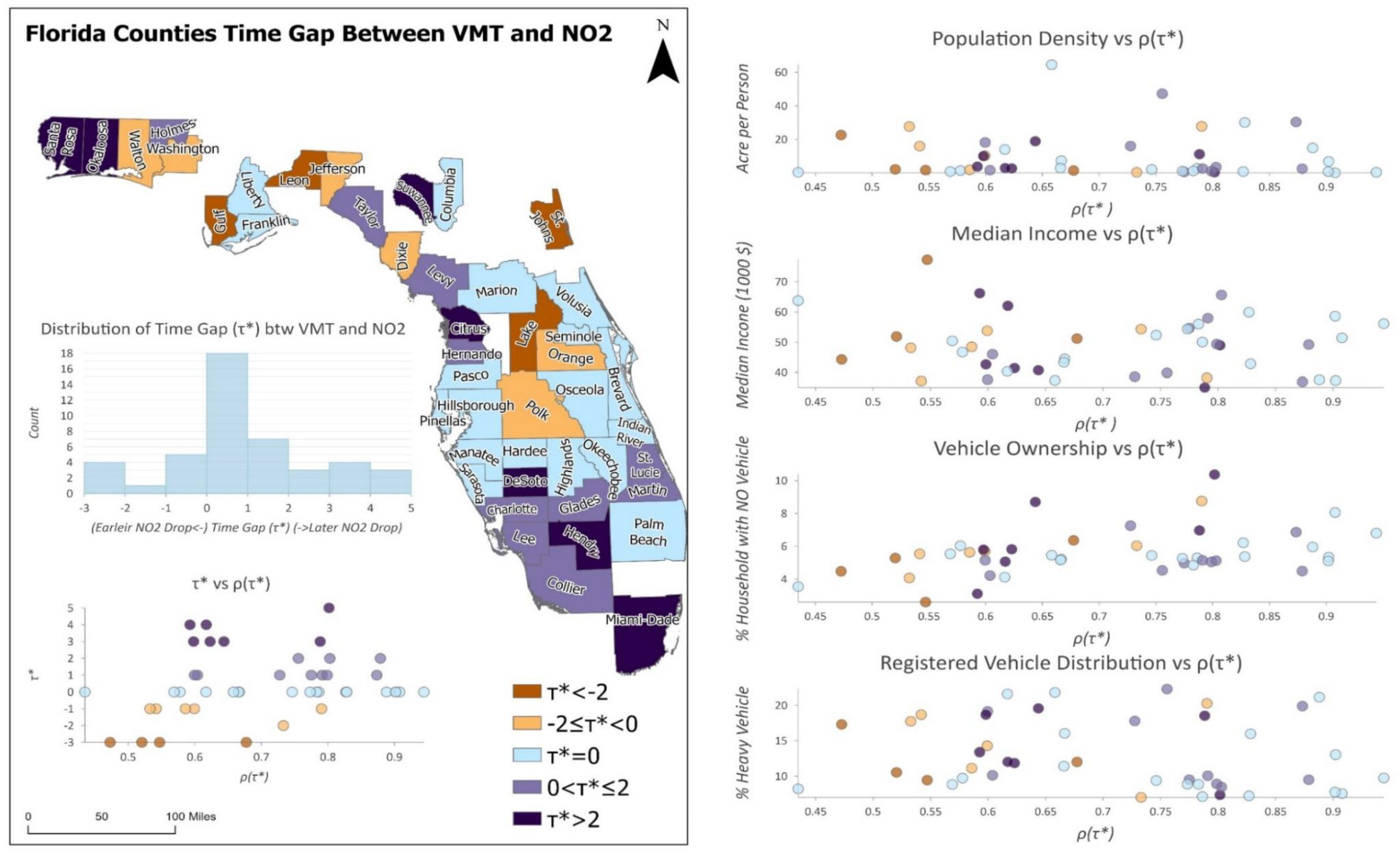
The map for time lag is presented in Figure 9 to illustrate the overall cross-correlation analysis results across Florida. In general, the counties in which the NO₂ decline was observed before the VMT decrease were clustered in the southern sections of the state whereas the counties where the NO₂ decrease was observed after VMT were located in the center and northern parts of the state. Additionally, the distribution for the time lag indicates that most of the counties observed the VMT and NO₂ concentration decreased on the same days. Furthermore, the scatter graphs for time lag $\left({\tau }^{\ast }\right)$ and maximum correlation $\rho \left({\tau }^{\ast }\right)$ indicates that the counties in which the NO₂ concentration decreased after the VMT (i.e., the counties with negative $\left({\tau }^{\ast }\right)$ value) presented a slightly less correlation compared to the counties with a positive $\left({\tau }^{\ast }\right)$ value. Counties without a time lag (${\tau }^{\ast }$= 0) indicate a higher variation on the correlation coefficient. This revealed that the effect of traffic on NO₂ concentration varies regardless of the time lag.

Additional to the population density and median income, registered heavy vehicle percentage and the percentage of the households with no vehicle for each county were also evaluated against the maximum correlation coefficient with different time lags. Surprisingly, a higher correlation was observed in the counties with higher percentage of households without a vehicle. This indicates that the increase on the households with no vehicle results in a higher correlation between VMT and NO₂. However, this can be negligible considering very low percentages on the zero-vehicle ownership.

To sum up, no significant impacts from the population, income, and vehicle distribution of county characteristics were observed on the time lag between VMT and NO₂. Future studies shall include the weather and commercial industry information from each county so that additional impacts on the relationship between VMT and NO₂ concentrations can be tested. Especially since the NO₂ production can also occur due to commercial manufacturing and food manufacturing, such information can help assess the time lags that occur in different counties.

4. Discussion

Previous studies have investigated the impact of COVID-19 response on air quality and found a significant improvement in several countries including India [11,28], Italy [27], Spain [29], and Kazakhstan [30]. The space agencies have also reported a significant improvement on the air quality by using remote sensing technologies [12,13,15]. This reduction on air pollution, however, was not observed in the U.S. cities Memphis [26] and New York City [42] concluding that the traffic related air pollutions (i.e., PM and NO₂) have not decreased compared both with previous years and the previous months in 2020. However, the study conducted in Memphis, TN analyzed only one ground station measurements for NO₂ and this station was not a near-roadway station. Additionally, the study conducted in New York City evaluated the measurements from only three ground stations for the NO₂ concentrations where two of those stations were in close proximity. On the other hand, another study [22] evaluated the measurements from all ground stations in the US and found an average of a 25% reduction on NO₂ concentrations compared to previous years. Additionally, another study using ground stations with nationwide coverage in the U.S. [24] visualized the abrupt reduction on PM and ozone compared to the previous years starting two weeks before the stay at home orders and converging back to the historical average shortly after the stay at home orders. NASA’s Scientific Visualization Studio, also, depicts a significant NO₂ reduction in East Coast regions of the U.S. by comparing the averages of 15 March–15 April 2020 to the averages of the same period from previous years This conflict in the studies analyzing the U.S. air quality with respect to the impact of COVID response raises a major issue that the air pollution depends on several local factors and not dependent only human activities and traffic. Thus, it is difficult to extract the COVID impact on air quality and more analyses is needed with more data including other environmental factors such as wind.

In this study, we focused on the immediate impact of the COVID-19, which started in 13 March and converged to a new normal by the end of the month as it can be observed from the national and statewide VMTs in Figure 4. Although the similar behavior between NO₂ and VMT during the immediate impact period could have been due to several reasons such as environmental conditions as stated in [43], it reveals valuable information in regard to the relationship between traffic and NO₂ concentrations. By using this information, our study confirmed that there was no significant delay on air quality improvement during or after a sharp decline in traffic.

On the other hand, this study had several limitations. First, we assumed that NO₂ distributes normally in each county and daily NO₂ concentration was calculated as the average of the pixel values that fell in the county. This can be negligible when it considered that there are only 11 surface measurement stations to observe NO₂ air pollution in Florida and those stations scattered around only the six most populated counties. Second, there are several factors that may affect the NO₂ concentrations such as wind, temperature, participation, industrial activities, coil burn for house heating, etc. However, we focused on the immediate impacts of COVID-19 to observe a specific time period where traffic substantially decreased. The strength of this study also lay on the relationship between traffic and NO₂ concentrations. To the best of author’s knowledge, this is the first study to quantify a time-lag between traffic and NO₂ concentrations and our methodology on extracting county level air quality information from Sentinel 5-P can be used to understand regional air quality trends where there is no surface station.

5. Conclusions

The impacts of COVID-19 and ensuing social distancing behaviors on traffic have enabled researchers to analyze an unprecedented experiment on air quality. This study particularly investigates the correlation and time lag between the traffic and NO₂ concentrations in all the Florida Counties through March 2020 when the immediate impacts of COVID-19 response were observed in the region. County level daily NO₂ concentrations were extracted from Sentinel-5P satellite, which expected to change the way the air quality is monitored today and vehicle mile traveled (VMT) estimates were acquired from cell phone mobility records. Population density, median income, and the percentage of the households with no vehicle are also obtained for each county from the US Census’s 2018 American Community Survey. A cross-correlation-based dependency analysis was conducted with the Pearson’s r statistic to analyze the similarities and associated time lag between 7-day moving averages of VMT and NO₂ concentration of 67 counties.

Among the 67 Florida Counties, an average of 54.07% and 59.68% decrease were observed for NO₂ and VMT, respectively. This decrease is higher compared to the previous studies since it indicates the percentage difference between the observed maximum and minimum values within the month of March 2020. However, findings indicate that social distancing behaviors have affected the traffic and air quality before the official policy enacted in Florida and this should be considered by further studies on the air quality impacts of COVID-19 to determine the study periods. Furthermore, majority of the counties have no time lag between VMT and NO₂ concentration; however, a cluster of South Florida counties presents an earlier decrease on NO₂ concentration compare to VMT. This indicates that the improvements on air quality among those southern counties are not transportation related and our investigation on socioeconomics factors such as population and income shows no significant impact on the time lag.

Future studies shall include the environmental conditions and information on the commercial industries from each county so that additional impacts on the relationship between VMT and NO₂ concentration can be tested. The proposed analysis can also be utilized if other pollutant data sets can be obtained for CO, CO₂, and particulate matter (PM). In addition, these results are very site specific, and therefore it would be interesting to study other states that had different experiences with COVID-19.

References

- WHO. Coronavirus Disease 2019—Situation Report—193; World Health Organization: Geneva, Switzerland, 2020. [Google Scholar]
- Wikipedia 2020 Stock Market Crash. Available online: https://en.wikipedia.org/wiki/2020_stock_market_crash (accessed on 10 July 2020).
- Cicala, S.; Holland, S.P.; Mansur, E.T.; Muller, N.Z.; Yates, A. Expected health effects of reduced air pollution from covid-19 social distancing. SSRN Electron. J. 2020, 61, 1–28. [Google Scholar] [CrossRef]
- Shilling, F. Special Report 3: Impact of COVID19 Mitigation on Traffic, Fuel Use and Climate Change; Road Ecology Center (REC): Davis, CA, USA, 2020. [Google Scholar]
- Reed, T. Understanding the Impact of COVID-19 on Commuting and Retail: An Analysis of the U.S. Epicenter. Available online: https://inrix.com/campaigns/coronavirus-impact-study/ (accessed on 13 July 2020).
- Unacast Social Distancing Scoreboard. Available online: https://www.unacast.com/covid19/social-distancing-scoreboard (accessed on 10 October 2020).
- StreetLight Data Inc. StreetLight’s VMT Data for All U.S. Counties. Available online: https://learn.streetlightdata.com/vmt-data-counties (accessed on 31 July 2020).
- Google Community Mobility Reports. Available online: https://www.google.com/covid19/mobility/ (accessed on 13 July 2020).
- Aloi, A.; Alonso, B.; Benavente, J.; Cordera, R.; Echániz, E.; González, F.; Ladisa, C.; Lezama-Romanelli, R.; López-Parra, Á.; Mazzei, V.; et al. Effects of the COVID-19 lockdown on urban mobility: Empirical evidence from the city of Santander (Spain). Sustainability 2020, 12, 3870. [Google Scholar] [CrossRef]
- Gillingham, K.T.; Knittel, C.R.; Li, J.; Ovaere, M.; Reguant, M. The short-run and long-run effects of Covid-19 on energy and the environment. Joule 2020, 4, 1337–1341. [Google Scholar] [CrossRef] [PubMed]
- Sharma, S.; Zhang, M.; Anshika; Gao, J.; Zhang, H.; Kota, S.H. Effect of restricted emissions during COVID-19 on air quality in India. Sci. Total Environ. 2020, 728, 138878. [Google Scholar] [CrossRef] [PubMed]
- Goldbaum, E. NASA Probes Environment, COVID-19 Impacts, Possible Links. Available online: https://www.nasa.gov/feature/nasa-probes-environment-covid-19-impacts-possible-links (accessed on 10 July 2020).
- Patel, K. Airborne Nitrogen Dioxide Plummets over China. Available online: https://earthobservatory.nasa.gov/images/146362/airborne-nitrogen-dioxide-plummets-over-china (accessed on 10 July 2020).
- Schindler, T.L. Reductions in Pollution Associated with Decreased Fossil Fuel Use Resulting from COVID-19 Mitigation. Available online: https://svs.gsfc.nasa.gov/4810 (accessed on 11 June 2020).
- NOAA. NOAA’s Polar-Orbiting Satellites See Drop in U.S. Air Pollution. Available online: https://www.nesdis.noaa.gov/content/noaa’s-polar-orbiting-satellites-see-drop-us-air-pollution (accessed on 28 July 2020).
- Zheng, Z.; Yang, Z.; Wu, Z.; Marinello, F. Spatial variation of NO2 and its impact factors in China: An application of sentinel-5P products. Remote Sens. 2019, 11, 1939. [Google Scholar] [CrossRef] [Green Version]
- USEPA. Reviewing National Ambient Air Quality Standards (NAAQS): Scientific and Technical Informatio, Table of Current NAAQS Table. Available online: https://www.epa.gov/criteria-air-pollutants/naaqs-table (accessed on 11 July 2020).
- Wikipedia National Ambient Air Quality Standards. Available online: https://en.wikipedia.org/wiki/National_Ambient_Air_Quality_Standards (accessed on 11 July 2020).
- USEPA. Nitrogen Dioxide (NO2) Pollution: Applying or Implementing Nitrogen Dioxide Standards. Available online: https://www.epa.gov/no2-pollution/applying-or-implementing-nitrogen-dioxide-standards#sip (accessed on 11 July 2020).
- Ialongo, I.; Virta, H.; Eskes, H.; Hovila, J.; Douros, J. Comparison of TROPOMI/Sentinel-5 Precursor NO2 observations with ground-based measurements in Helsinki. Atmos. Meas. Tech. 2020, 13, 205–218. [Google Scholar] [CrossRef] [Green Version]
- United States Census Bureau. American Community Survey (ACS). Available online: https://www.census.gov/acs/www/data/data-tables-and-tools/data-profiles/ (accessed on 31 July 2020).
- Berman, J.D.; Ebisu, K. Changes in U.S. air pollution during the COVID-19 pandemic. Sci. Total Environ. 2020, 739, 139864. [Google Scholar] [CrossRef] [PubMed]
- OpenAQ. Available online: https://openaq.org (accessed on 31 July 2020).
- Bekbulat, B.; Apte, J.S.; Millet, D.B.; Robinson, A.; Wells, K.C.; Marshall, J.D. PM2.5 and ozone air pollution levels have not dropped consistently across the US following societal Covid response. ChemRxiv 2020, 1–26. [Google Scholar] [CrossRef]
- USEPA. Outdoor Air Quality Data. Available online: https://www.epa.gov/outdoor-air-quality-data/download-daily-data (accessed on 31 July 2020).
- Jia, C.; Fu, X.; Bartelli, D.; Smith, L. Insignificant impact of the “stay-at-home” order on ambient air quality in the Memphis Metropolitan Area, U.S.A. Atmosphere 2020, 11, 630. [Google Scholar] [CrossRef]
- Collivignarelli, M.C.; Abbà, A.; Bertanza, G.; Pedrazzani, R.; Ricciardi, P.; Carnevale Miino, M. Lockdown for CoViD-2019 in Milan: What are the effects on air quality? Sci. Total Environ. 2020, 732, 139280. [Google Scholar] [CrossRef] [PubMed]
- Mahato, S.; Pal, S.; Ghosh, K.G. Effect of lockdown amid COVID-19 pandemic on air quality of the megacity Delhi, India. Sci. Total Environ. 2020, 730, 139086. [Google Scholar] [CrossRef] [PubMed]
- Baldasano, J.M. COVID-19 lockdown effects on air quality by NO2 in the cities of Barcelona and Madrid (Spain). Sci. Total Environ. 2020, 741, 140353. [Google Scholar] [CrossRef] [PubMed]
- Kerimray, A.; Baimatova, N.; Ibragimova, O.P.; Bukenov, B.; Kenessov, B.; Plotitsyn, P.; Karaca, F. Assessing air quality changes in large cities during COVID-19 lockdowns: The impacts of traffic-free urban conditions in Almaty, Kazakhstan. Sci. Total Environ. 2020, 730, 139179. [Google Scholar] [CrossRef] [PubMed]
- Center for Disease Control and Prevention. People at Increased Risk and Other People Who Need to Take Extra Precautions. Available online: https://www.cdc.gov/coronavirus/2019-ncov/need-extra-precautions/index.html (accessed on 31 July 2020).
- Kaya, K.; Gündüz Öğüdücü, Ş. Deep Flexible Sequential (DFS) Model for Air Pollution Forecasting. Sci. Rep. 2020, 10, 3346. [Google Scholar] [CrossRef] [PubMed]
- Veefkind, J.P.; Aben, I.; McMullan, K.; Förster, H.; de Vries, J.; Otter, G.; Claas, J.; Eskes, H.J.; de Haan, J.F.; Kleipool, Q.; et al. TROPOMI on the ESA Sentinel-5 Precursor: A GMES mission for global observations of the atmospheric composition for climate, air quality and ozone layer applications. Remote Sens. Environ. 2012, 120, 70–83. [Google Scholar] [CrossRef]
- Sentinel Online. Sentinel-5P. Available online: https://sentinel.esa.int/web/sentinel/missions/sentinel-5p (accessed on 31 July 2020).
- European Space Agency (ESA). Copernicus Open Access Hub. Available online: https://scihub.copernicus.eu/ (accessed on 30 July 2020).
- Eskes, H.; Van Geffen, J.; Boersma, F.; Eichmann, K.-U.; Apituley, A.; Pedergnana, M.; Sneep, M.; Veefkind, J.P.; Loyola, D. Sentinel-5 Precursor/TROPOMI Level 2 Product User Manual Nitrogendioxide; Royal Dutch Meteorological Institute: De Bilt, The Netherlands, 2019. [Google Scholar]
- StreetLight Data Inc. Our Methodology and Data Sources StreetLight InSight® Metrics: Our Methodology and Data Sources; StreetLight Data Inc.: Richmond, VA, USA, 2020. [Google Scholar]
- StreetLight Data Inc. VMT Monitor Methodology and Validation; StreetLight Data Inc.: Richmond, VA, USA, 2020; pp. 1–15. [Google Scholar]
- Rao, K.D.; Swamy, M.N.S.; Rao, K.D.; Swamy, M.N.S. Spectral analysis of signals. Digit. Signal Process. 2018, 721–751. [Google Scholar] [CrossRef]
- Wikipedia Cross-Corelation. Available online: https://en.wikipedia.org/wiki/Cross-correlation (accessed on 30 July 2020).
- Wikipedia COVID-19 Pandemic in Florida. Available online: https://en.wikipedia.org/wiki/COVID-19_pandemic_in_Florida (accessed on 30 July 2020).
- Zangari, S.; Hill, D.T.; Charette, A.T.; Mirowsky, J.E. Air quality changes in New York City during the COVID-19 pandemic. Sci. Total Environ. 2020, 742, 140496. [Google Scholar] [CrossRef] [PubMed]
- Wang, P.; Guo, H.; Hu, J.; Kota, S.H.; Ying, Q.; Zhang, H. Responses of PM2.5 and O3 concentrations to changes of meteorology and emissions in China. Sci. Total Environ. 2019, 662, 297–306. [Google Scholar] [CrossRef] [PubMed]
Figure 1.
Study area.
Figure 2.
Flowchart for extracting daily NO2 concentration for each county in Florida.
Figure 3.
Examples of Sentinel-5P daily measurement for NO2 densities over Florida.
Figure 4.
Seven day moving averages of vehicle mile traveled (VMT) in the U.S. (a) Seven day moving averages of VMT and NO2 concentration in Florida (b).
Figure 5.
Distribution of % decrease on VMT and NO2 concentrations among Florida counties.
Figure 6.
Date on which maximum and minimum values were observed for 7-day moving averages of VMT and NO2 concentrations among Florida counties.
Figure 7.
Different time lags and correlation between 7-day moving averages of VMT and NO2 in counties with high population density (left column <0.5 acre per person) and low population density (right column >2 acre per person).
Figure 8.
Different time lags and correlation between 7-day moving averages of VMT and NO2 in counties with higher median income (left column > $55,000) and lower median income (right column < $40,000).
Figure 9.
Distribution of the time lag between VMT and NO2 concentration among Florida counties and potential factors that can affect the correlation between VMT and NO2 concentration.
Publisher’s Note: MDPI stays neutral with regard to jurisdictional claims in published maps and institutional affiliations. |
© 2020 by the authors. Licensee MDPI, Basel, Switzerland. This article is an open access article distributed under the terms and conditions of the Creative Commons Attribution (CC BY) license (http://creativecommons.org/licenses/by/4.0/).
Share and Cite
MDPI and ACS Style
Karaer, A.; Balafkan, N.; Gazzea, M.; Arghandeh, R.; Ozguven, E.E. Analyzing COVID-19 Impacts on Vehicle Travels and Daily Nitrogen Dioxide (NO2) Levels among Florida Counties. Energies 2020, 13, 6044. https://doi.org/10.3390/en13226044
AMA Style
Karaer A, Balafkan N, Gazzea M, Arghandeh R, Ozguven EE. Analyzing COVID-19 Impacts on Vehicle Travels and Daily Nitrogen Dioxide (NO2) Levels among Florida Counties. Energies. 2020; 13(22):6044. https://doi.org/10.3390/en13226044
Chicago/Turabian StyleKaraer, Alican, Nozhan Balafkan, Michele Gazzea, Reza Arghandeh, and Eren Erman Ozguven. 2020. "Analyzing COVID-19 Impacts on Vehicle Travels and Daily Nitrogen Dioxide (NO2) Levels among Florida Counties" Energies 13, no. 22: 6044. https://doi.org/10.3390/en13226044
Note that from the first issue of 2016, this journal uses article numbers instead of page numbers. See further details here.