Study of Dynamics of a COVID-19 Model for Saudi Arabia with Vaccination Rate, Saturated Treatment Function and Saturated Incidence Rate

Abstract

This paper proposes, validates and analyzes the dynamics of the susceptible exposed infectious recovered (SEIR) model for the propagation of COVID-19 in Saudi Arabia, which recorded the largest number of cases in the Arab world. The model incorporates a saturated incidence rate, a constant vaccination rate and a nonlinear treatment function. The rate of treatment is assumed to be proportional to the number of infected persons when this number is low and reaches a fixed value for large number of infected individuals. The expression of the basic reproduction number is derived, and the model basic stability properties are studied. We show that when the basic reproduction number is less than one the model can predict both a Hopf and backward bifurcations. Simulations are also provided to fit the model to COVID-19 data in Saudi Arabia and to study the effects of the parameters of the treatment function and vaccination rate on disease control.

1. Introduction

Multiple waves of COVID-19 are still attacking many countries around the world. The severity of the pandemic is accentuated by the emergence of new and more contagious strains of the virus. Many countries are still struggling to vaccinate their population in order to curve the waves of infections and reduce the hospitalizations that have affected their health systems. The use of mathematical models to predict disease transmission is useful for analysis and prediction particularly when the model is validated against the available disease data.

A mathematical model can predict future situations of the disease spread and evaluate the best strategy to be invoked depending on the epidemiological situation. Since the outbreak of the disease, there have been a large number of studies [1,2,3,4,5,6,7,8,9] that used compartment models based on SIR (susceptible (S), infectious (I) and recovered (R)) and SEIR (susceptible (S), exposed (E), infectious (I) and recovered (R)) epidemic models to predict the spread of the disease.

These models consist generally of deterministic ordinary differential equations or difference equations and are amenable sometimes to analytical manipulations that can extract some important parameters, such as the basic reproduction number that can quantify the spread of the disease. These models are also flexible. They can accommodate a variety of expressions for incidence rate [1], can include the effect of a variable recovery rate [2] and can simulate various scenarios of pandemic management, such as lockdown [3,4], closure of sectors of the economy, compliance of people with protection measures [4], social distancing [5], travel restrictions [6], media coverage [7], quarantine [8], super-spreaders individuals [9] and vaccination [10,11,12]. Once validated, these models can be used as a public health decision support tool [4].

In this paper, we develop, validate and examine the dynamics of a SEIR model for COVID-19. The proposed model includes a number of characteristics. In many epidemic models, the bilinear incidence rate $\beta SI$ is used. In this paper, we adopt a nonlinear expression of the incidence rate $\beta SI/(1+\alpha I)$ that includes an inhibition $1/(1+\alpha I)$ effect reflecting the behavior of susceptible persons as the infection spreads. This form of incidence rate was shown to be more realistic than the bilinear incidence expression [1]. The proposed model also includes a treatment function. A number of epidemic models considered the treatment rate to be proportional to the number of infected persons. However, the recovery rate is known to be strongly dependent on health resources and the treatment efficiency. Since, generally, the treatment capacity of each country is limited, it seems logical to consider a more realistic treatment function. Various expressions for treatment functions have been proposed in the literature [13,14,15,16,17]. Here, we adopt the saturated treatment $cI/(1+bI)$ function suggested by Zhang and Liu [17]. This form has the advantage of producing a constant value when the number of infected persons (I) is very low and reaches an asymptotic constant value if the number of infected individuals is large. Furthermore, this form of treatment function has a finite and continuous value. The model also includes a vaccination rate. Vaccine administration is a highly effective method of preventing and reducing viral infections [18]. Vaccination and optimal control are the key points to controlling an epidemic situation as discussed in [11,19,20,21], and the majority of countries have embarked on aggressive vaccination campaigns against COVID-19.

The novelty in the proposed SEIR model is that it includes a saturated incidence rate and a saturated treatment function in addition to a vaccination rate. Some models in the literature either included some of these elements or included all of these elements but not in the current expressions adopted in this paper. Zhang et al. [16], for instance, included, in their SEIR model, all the elements except the vaccination rate. Annas [10], in their study of the spread of the disease in Indonesia included, in their SEIR model, all the aforementioned elements except the treatment function. Deng et al. [22], proposed a non-smooth Filippov epidemic system to examine the effects of some control strategies, such as media coverage, treatment and vaccination. However, the authors considered only a SIR and not a SEIR model.

In the first step of our analysis, the model is validated using real COVID-19 data in Saudi Arabia. This allows the extraction of a number of model parameters. In the next step, simulations are carried out to study the bifurcation behavior of the model using the basic reproduction number as the main bifurcation parameter. A numerical sensitivity analysis is also performed for the effect of model parameters associated with the treatment function and the vaccination rate.

The organization of the rest of the paper is as follows. In Section 2, we present and explain the model. Then, in Section 3, we prove the model positivity and boundedness of its solutions and derive the expression of the basic reproduction number. In Section 4, the backward bifurcation is examined. Section 5 of the paper includes numerical simulations to support the theoretical proofs.

2. The Model

The proposed SEIR model for COVID-19 transmission is composed of four compartments—namely, susceptible (S), exposed (E), infected (I) and recovered individuals (R). The changes that occur in each compartment can be interpreted by Figure 1. The model consists of the following ordinary differential equations,

$$\begin{array}{cc}\hfill \frac{dS}{dt}=& A-\mu S-\frac{\alpha IS}{(1+{\alpha }_{1}I)}-vS\hfill \end{array}$$

(1)

$$\begin{array}{cc}\hfill \frac{dE}{dt}=& \frac{\alpha IS}{(1+{\alpha }_{1}I)}-(\beta +\mu )E;\hfill \end{array}$$

(2)

$$\begin{array}{cc}\hfill \frac{dI}{dt}=& \beta E-(\epsilon +\delta +\mu )I-\frac{cI}{(1+bI)}\hfill \end{array}$$

(3)

$$\begin{array}{cc}\hfill \frac{dR}{dt}=& \delta I-\mu R+\frac{cI}{(1+bI)}+vS.\hfill \end{array}$$

(4)

A is the population recruitment rate, $\mu$ is the population natural death rate per time, and $\alpha$ is the transmission rate. The term $\frac{1}{1+{\alpha }_{1}I}$ reflects the inhibitory effect from the behavioral change of the susceptible when the number of incidence increases. $\beta$ is the rate of transformation to infective persons, $\delta$ is the natural recovery rate of the infected persons, $\epsilon$ is the mortality due to the disease, and v is the rate of vaccination of susceptible population.

The term $T\left(I\right)=\frac{cI}{(1+bI)}$ represents the treatment function where b represents the saturation factor measuring the effect of the infected individual when delayed for treatment, and c is the maximal supplied medical resources. $T\left(I\right)$ can be seen to approach $cI$ when I is small; On the other hand, $T\left(I\right)$ approaches $c/b$ when I is large. It should be noted that, compared to other forms proposed in the literature [13,14,15], this form of treatment function has also the advantage of being continuous and differential.

3. Model Analysis

3.1. Positivity of the Model Solutions

Theorem 1.

Let $S_0,E_0,I_0,R_0\ge 0$. The solutions of Equations (1)–(4) with initial conditions $\left(S\right(0),E(0),$$I\left(0\right),R\left(0\right))=(S_0,E_0,I_0,R_0)$ are non-negative for $t>0$.

Proof. 

The proof follows the general approach used by a number of authors, including [23]. We have from (Equation (1)) that,

$$\begin{array}{cc}\hfill \frac{dS\left(t\right)}{dt}& =A-S\left(t\right)w\left(t\right),\hfill \end{array}$$

(5)

where

$$\begin{array}{c}\hfill w\left(t\right)=\mu +\alpha I/(1+{\alpha }_{1}I)+v.\end{array}$$

Integrating Equation (5) yields

$$\begin{array}{c}\hfill S\left(t\right)=\left({\int }_0^{t}A{\mathrm{e}}^{{\int }_0^{\tau }w\left(u\right)\mathrm{d}u}\mathrm{d}\tau +{\mathit{S}}_0\right){\mathrm{e}}^{-{\int }_0^{t}w\left(\tau \right)\mathrm{d}\tau }>0.\end{array}$$

Thus, $S\left(t\right)>0$ for all t.

For the proofs that $E\left(t\right)$ and $I\left(t\right)$ are positive, we divide this issue into four cases:

• $E_0=I_0=0$. From Equations (2) and (3), we can see $E\left(t\right)=I\left(t\right)=0$ for all $t\ge 0$.
• $E_0>0$ and $I_0=0$. Since $E\left(t\right)$ is continuous at $t=0$ and since $\frac{dI}{dt}(t=0)=\beta E_0>0$, we can conclude that $E\left(t\right)>0$ and $I\left(t\right)>0$ for all $t\ge 0$. If this is not true, then we can choose

  $$\begin{array}{c}\hfill t_1=inf\left\{t:E\left(t\right)=0\mathrm{or}I\left(t\right)=0\right\}\in (0,\infty ).\end{array}$$
  If $E\left(t_1\right)=0$, then since $\frac{dE}{dt}\ge -(\beta +\mu )E_0$ for $0\le t\le t_1$, we conclude that

  $$\begin{array}{c}\hfill E\left(t_1\right)\ge E_0{\mathrm{e}}^{-(\beta +\mu )t_1}>0,\end{array}$$

  (6)

  which contradicts the assumption that $E\left(t_1\right)=0$.
  If, on the other hand, $I\left(t_1\right)=0$, then there exists $\theta$ such that $t_1>\theta$ and $0<I\left(t\right)<\psi$ on $[t_1-\theta ,t_1)$. Therefore, Equation (3) implies that

  $$\begin{array}{c}\hfill \frac{dI}{dt}\ge -\left((\epsilon +\delta +\mu )+\frac{c}{1+bI}\right)I.\end{array}$$

  (7)
  This gives

  $$\begin{array}{c}\hfill I\left(t_1\right)\ge I(t_1-\theta ){\mathrm{e}}^{-{\int }_{(t_1-\theta )}^{t_1}\left((\epsilon +\delta +\mu )+\frac{c}{1+bI\left(u\right)}\right)du}>0,\end{array}$$

  (8)

  which also contradicts the assumption that $I\left(t_1\right)=0$. The same analysis can be carried out for the other cases: $(E_0=0,I_0>0)$ and $(E_0>0,I_0>0)$.

We conclude, therefore, that $E\left(t\right)$ and $I\left(t\right)$ are positive for all $t\ge 0$.

Next, since we have shown that $S\left(t\right)>0$ and $I\left(t\right)>0$, we can deduce from Equation (4) that

$$\begin{array}{cc}\hfill -\frac{dR\left(t\right)}{dt}& \le \mu R\left(t\right).\hfill \end{array}$$

(9)

Applying Grönwall’s lemma [24] to Equation (9) with initial condition $R_0$ yields,

$$\begin{array}{cc}\hfill -R\left(t\right)& \le -R_0{\mathrm{e}}^{-{\int }_0^t\left(\mu \right)d\tau }<0.\hfill \end{array}$$

This proves that $R\left(t\right)>0$. □

3.2. Boundedness

Theorem 2.

The compact set Ψ defined by

$$\begin{array}{cc}\hfill \Psi =& \{(S\left(t\right),E\left(t\right),I\left(t\right),R\left(t\right))\in {\mathrm{I}\mathrm{R}}_{+}^4,S\left(t\right)+E\left(t\right)+I\left(t\right)+R\left(t\right)\le \frac{A}{\mu }\},\hfill \end{array}$$

(10)

where ($S\left(t\right),E\left(t\right),I\left(t\right),R\left(t\right)$) are the solutions of the model (Equations (1)–(4)) with initial conditions ($S_0,E_0,I_0,R_0$) is a positively invariant region.

Proof. 

Denote by $N\left(t\right)=S\left(t\right)+E\left(t\right)+I\left(t\right)+R\left(t\right)$, and then we have

$$\begin{array}{cc}\hfill \frac{dN\left(t\right)}{dt}=& -N\left(t\right)\mu -\epsilon \mathit{I}+A,\hfill \end{array}$$

(11)

$$\begin{array}{cc}\hfill \frac{dN\left(t\right)}{dt}\le & -N\left(t\right)\mu +A.\hfill \end{array}$$

(12)

Therefore,

$$\begin{array}{cc}\hfill N\left(t\right)& \le \left(N\left(0\right)exp(-\mu t)+\frac{A}{\mu }(1-exp(-\mu t))\right),\hfill \end{array}$$

(13)

where $N\left(0\right)$ is the initial condition of $N\left(t\right)$. Therefore, $0<N\left(t\right)<\frac{A}{\mu }$ as t goes to $+\infty$ and $\frac{dN\left(t\right)}{dt}<0$ for $N>\frac{A}{\mu }$. This shows that $\Psi$ is positively invariant. □

4. Existence of Equilibria, Stability and Bifurcation Analysis

In the rest of analysis, we consider only Equations (1)–(3), since they do not depend on the variable R. The disease-free equilibrium ${\mathcal{E}}_0(S,E,I)=(\frac{A}{\mu +v},0,0)$ is always a solution of the model. The non-trivial solutions are obtained by considering the steady state of Equations (1)–(3), which yields:

$$\begin{array}{cc}\hfill S& =\frac{\mathit{A}}{\mu +v}-I\left[\frac{c\left(\mu +\beta \right)}{\left(\mathit{I}b+1\right)\beta \left(\mu +v\right)}+\frac{\left(\epsilon +\delta +\mu \right)\left(\mu +\beta \right)}{\beta \left(\mu +v\right)}\right],\hfill \end{array}$$

(14)

$$\begin{array}{cc}\hfill E& =I\left[\frac{c}{\beta \left(\mathit{I}b+1\right)}+\frac{\left(\epsilon +\delta +\mu \right)}{\beta }\right].\hfill \end{array}$$

(15)

where I is the positive root of the quadratic equation,

$$\begin{array}{cc}\hfill {\mathcal{E}}_1\left(I\right)=& a_2{I}^2+a_{1}I+a_0=0,\hfill \end{array}$$

(16)

where $a_0$, $a_1$ and $a_2$ are defined by

$$\begin{array}{cc}\hfill a_2& =\left(\mu +v\right)\left(\epsilon +\delta +\mu \right)\left(\mu +\beta \right)b{\alpha }_1+b\left(\epsilon +\delta +\mu \right)\left(\mu +\beta \right)\alpha >0,\hfill \\ \hfill a_1& =-\alpha b\beta \mathit{A}+\left(\mu +v\right)\left(\epsilon +\delta +\mu \right)\left(\mu +\beta \right)b+\left(\mu +\beta \right)\left({\alpha }_1\mu +\alpha 1v+\alpha \right)\left(c+\delta +\mu +\epsilon \right),\hfill \\ \hfill a_0& =--\left(\mu +v\right)\left(\mu +\beta \right)\left({\mathcal{R}}_0-1\right)\left(c+\delta +\mu +\epsilon \right).\hfill \end{array}$$

In these equations, ${\mathcal{R}}_0$ is the basic reproduction number, obtained with the techniques in [25]:

$$\begin{array}{c}\hfill {\mathcal{R}}_0=\frac{\mathit{A}\alpha \beta }{\left(\mu +v\right)\left(\mu +\beta \right)\left(c+\delta +\mu +\epsilon \right)}.\end{array}$$

(17)

Let $\Delta$ be the discriminant of the quadratic Equation (16). Solving for $\Delta =0$ in terms of ${\mathcal{R}}_0$, we find ${\mathcal{R}}_0={\mathcal{R}}_0^c$, where

$$\begin{array}{c}\hfill {\mathcal{R}}_0^c=1-1/4\frac{{{\mathit{a}}_1}^2}{b\left(\epsilon +\delta +\mu \right){\left(\mu +\beta \right)}^2\left({\alpha }_1\mu +{\alpha }_{1}v+\alpha \right)\left(\mu +v\right)\left(c+\delta +\mu +\epsilon \right)}.\end{array}$$

(18)

Thus, we have $\Delta <0⟺{\mathcal{R}}_0<{\mathcal{R}}_0^c<1,$ $\Delta =0⟺{\mathcal{R}}_0={\mathcal{R}}_0^c,$ $\Delta >0⟺{\mathcal{R}}_0>{\mathcal{R}}_0^c.$

The existence of the equilibrium can be analyzed by the following results:

1

Case $b=0$: Equation (16) has a unique solution $I=-a_0/a_1$. In this case, the Equations (1)–(3) has a unique steady state solution whenever ${\mathcal{R}}_0>1$ and no steady state solution if ${\mathcal{R}}_0\le 1$.

2

Case $b>0$:

(a)

Equations (1)–(3) have a unique steady state solution whenever ${\mathcal{R}}_0>1$;

(b)

Equations (1)–(3) have a unique steady state solution if ${\mathcal{R}}_0=1$ and $a_1<0$;

(c)

Equations (1)–(3) have a unique steady state solution of multiplicity 2 when ${\mathcal{R}}_0={\mathcal{R}}_0^c$ and $a_1<0$;

(d)

Equations (1)–(3) have two steady state solutions when ${\mathcal{R}}_0^c<{\mathcal{R}}_0<1$ and $a_1<0$.

(e)

Equations (1)–(3) have no steady state solution whenever ${\mathcal{R}}_0<{\mathcal{R}}_0^c$ and $a_1<0$ or whenever ${\mathcal{R}}_0\le 1$ and $a_1>0$.

4.1. Local Stability Analysis of the Disease-Free Solution

In this part of the paper, the local stability of the disease-free solution is studied using the eigenvalues of the Jacobian matrices of (1)–(3) at the disease-free equilibrium ${\mathcal{E}}_0$. Thus, we have

$$\begin{array}{cc}\hfill \mathrm{J}({\mathcal{E}}_0)& =\left[\begin{array}{ccc}-\mu -v& 0& -\frac{\mathit{A}\alpha }{\mu +v}\\ 0& -\beta -\mu & \frac{\mathit{A}\alpha }{\mu +v}\\ 0& \beta & -\epsilon -\delta -\mu -c\end{array}\right].\hfill \end{array}$$

(19)

The eigenvalues of Jacobian matrices J(${\mathcal{E}}_0$) are:

$${\lambda }_i=\left[\begin{array}{c}-[\mu +v]\\ {\lambda }_2\\ {\lambda }_3\end{array}\right],$$

(20)

with

$$\begin{array}{cc}\hfill {\lambda }_2=& \frac{1}{2(\mu +v)}\left[-\left(\mu +v\right)\left(2\mu +c+\beta +\delta +\epsilon \right)+\sqrt{{\rm Y}}\right],\hfill \\ \hfill {\lambda }_3=& \frac{1}{2(\mu +v)}\left[-\left(\mu +v\right)\left(2\mu +c+\beta +\delta +\epsilon \right)-\sqrt{{\rm Y}}\right]<0,\hfill \\ \hfill {\rm Y}=& 4{\left(\mu +v\right)}^2\left(\mu +\beta \right)\left(\epsilon +\delta +\mu +c\right){\mathcal{R}}_0+{\left(\mu +v\right)}^2{\left(c-\beta +\delta +\epsilon \right)}^2>0.\hfill \end{array}$$

By simple Algebraic calculation, we have ${\lambda }_2=0$ when ${\mathcal{R}}_0=1$, ${\lambda }_2<0$ for ${\mathcal{R}}_0<1$ and ${\lambda }_2>0$ when ${\mathcal{R}}_0>1$. Therefore, the following result is obtained:

Lemma 1.

The disease-free equilibrium ${\mathcal{E}}_0$ is locally asymptotically stable if ${\mathcal{R}}_0<1$ and unstable if ${\mathcal{R}}_0>1$.

4.2. Backward Bifurcation

Theorem 3.

Equations (1)–(3) predict a backward bifurcation if $b>b_{1,cr}=\frac{\left(\epsilon +\delta +\mu +c\right){\alpha }_1}{c}+\frac{\left(\mu +\beta \right){\left(\epsilon +\delta +\mu +c\right)}^2}{\beta \mathit{A}c}$ and no backward bifurcation otherwise.

Proof. 

We consider the methodology detailed in [26] to prove the existence of a backward bifurcation. We define new variables: $x_1=S,x_2=E,x_3=I$. We can rewrite Equations (1)–(3) as,

$$\begin{array}{cc}\hfill \frac{d{x}_1}{dt}=f_1=& A-\mu x_1-\alpha x_3{x}_1/(1+{\alpha }_1{x}_3)-v{x}_1\hfill \end{array}$$

(21)

$$\begin{array}{cc}\hfill \frac{d{x}_2}{dt}=f_2=& \alpha x_3{x}_1/(1+{\alpha }_1{x}_3)-(\beta +\mu )x_2\hfill \end{array}$$

(22)

$$\begin{array}{cc}\hfill \frac{d{x}_3}{dt}=f_3=& \beta x_2-(\epsilon +\delta +\mu )x_3-c{x}_3/(1+b{x}_3).\hfill \end{array}$$

(23)

Let us assume $\alpha$ to be the bifurcation parameter. The condition ${\mathcal{R}}_0=1$ leads to

$$\begin{array}{cc}\hfill \alpha =& \frac{\left(\epsilon +\delta +\mu +c\right)\left(\mu +\beta \right)\left(\mu +v\right)}{\mathit{A}\beta }:={\alpha }^{*}.\hfill \end{array}$$

(24)

The Jacobian matrix of (21)–(23) at ${\mathcal{E}}_0$ when $\alpha ={\alpha }^{*}$ is

$$\begin{array}{c}\hfill J=\left[\begin{array}{ccc}-\mu -v& 0& -\frac{\left(\epsilon +\delta +\mu +c\right)\left(\mu +\beta \right)}{\beta }\\ 0& -\beta -\mu & \frac{\left(\epsilon +\delta +\mu +c\right)\left(\mu +\beta \right)}{\beta }\\ 0& \beta & -\epsilon -\delta -\mu -c\end{array}\right].\end{array}$$

(25)

The right eigenvector of the Jacobian matrix for the zero eigenvalue is

$$\begin{array}{c}\hfill (w_1,w_2,w_3)=\left[\begin{array}{c}-\frac{\left(\epsilon +\delta +\mu +c\right)\left(\mu +\beta \right)}{\beta \left(\mu +v\right)}\\ \frac{\epsilon +\delta +\mu +c}{\beta }\\ 1\end{array}\right].\end{array}$$

(26)

The left eigenvector is $(v_1,v_2,v_3)$ = $(0,\frac{\beta }{\mu +\beta },1)$. The two stability parameters $\mathbf{a}$ and $\mathbf{b}$ [26] that define the conditions for the appearance of a backward bifurcation are:

$$\begin{array}{cc}\hfill \mathbf{a}=& \sum _{k,i,j=1}^3{v}_k{w}_i{w}_j\frac{{\partial }^2{f}_k}{\partial x_i\partial x_j},\hfill \end{array}$$

(27)

which yields

$$\begin{array}{c}\hfill \mathbf{a}=-2\frac{\left(\mu +\beta \right){\left(\epsilon +\delta +\mu +c\right)}^2}{\beta \mathit{A}}+2cb-2\left(\epsilon +\delta +\mu +c\right){\alpha }_1.\end{array}$$

The other parameter $\mathbf{b}$ is:

$$\begin{array}{c}\hfill \mathbf{b}=\sum _{k,i=1}^3{v}_k{w}_i\frac{{\partial }^2{f}_k}{\partial x_i\partial \alpha },\end{array}$$

(28)

which is reduced to

$$\begin{array}{c}\hfill \mathbf{b}=\frac{\beta \mathit{A}}{\left(\mu +\beta \right)\left(\mu +v\right)}>0.\end{array}$$

(29)

Since $\mathbf{b}$ is always positive, a backward bifurcation exists when

$$\begin{array}{c}\hfill \mathbf{a}>0\to b>b_{cr}=\frac{\left(\epsilon +\delta +\mu +c\right){\alpha }_1}{c}+\frac{\left(\mu +\beta \right){\left(\epsilon +\delta +\mu +c\right)}^2}{\beta \mathit{A}c}.\end{array}$$

(30)

□

5. Numerical Simulations

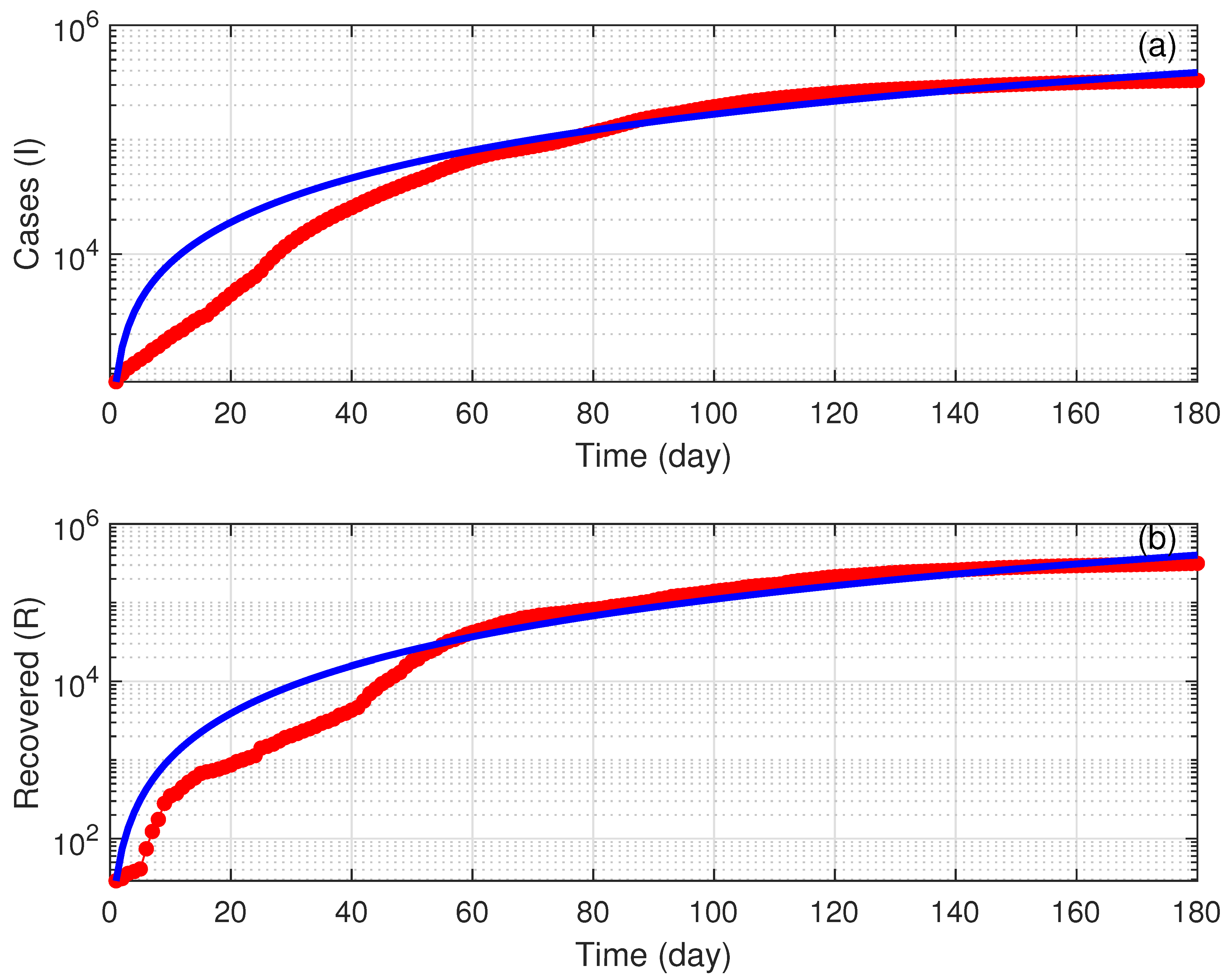
The first step in numerical simulations is to extract fitted values of model parameters using COVID-19 data for Saudi Arabia, a country with a population of 34,800,000 that reported 543,000 cases by the first of September 2021 [27]. The following model parameters were assumed to have constant and known values. These are the recruitment rate $A=1252$ and the natural death rate $\mu =4.21\times {10}^{-5}$ [28]. The death rate due to the disease is taken to be $\epsilon =0.012$ [27]. The other model parameters $({\alpha }_1,\beta ,\delta ,b,c)$ were fitted to the COVID-19 data, which are freely available on the Saudi Ministry of Health website [27].

The fitting task was achieved using (FMINCON), a MATLAB optimization software. FMINCON is used to find minimum of a constrained nonlinear multivariable function using a sequential quadratic programming (SQP) method. The fitting was done for a six month period starting from 24 March 2020. During this period, the vaccination campaign had not started yet, and thus the vaccination rate was taken to be zero. Figure 2 shows the results of fitting both infectious cases (I) and recovered cases (R). The fitting seems reasonable especially after an initial period of time.

Table 1. Parameters of the model.

Parameter	Value	Source
$\delta$	0.0078	fitted
$\beta$	$0.998$	fitted
A	1252	[28]
${\alpha }_1$	0.0179	fitted
$\epsilon$	$0.0012$	[27]
$\mu$	$4.21\times {10}^{-5}$	[27]
b	0.0376	fitted
c	0.4127	fitted

summarizes the obtained values of the fitted parameters. Using the fitted values (Table 1), we obtain a basic reproduction number of 1.87.

Next, numerical results are shown for the bifurcation behavior of the model using ${\mathcal{R}}_0$ as the main bifurcation parameter. The numerical analysis of the model is carried out using the software AUTO [29]. AUTO can be used to solve continuation and bifurcation problems in ordinary differential equations. These include continuation of equilibria and periodic orbits. First, it can be noted that using the values of Table 1 yields the following condition $b>b_{cr}=0.0186$ (Equation (30)) for the emergence of a backward bifurcation.

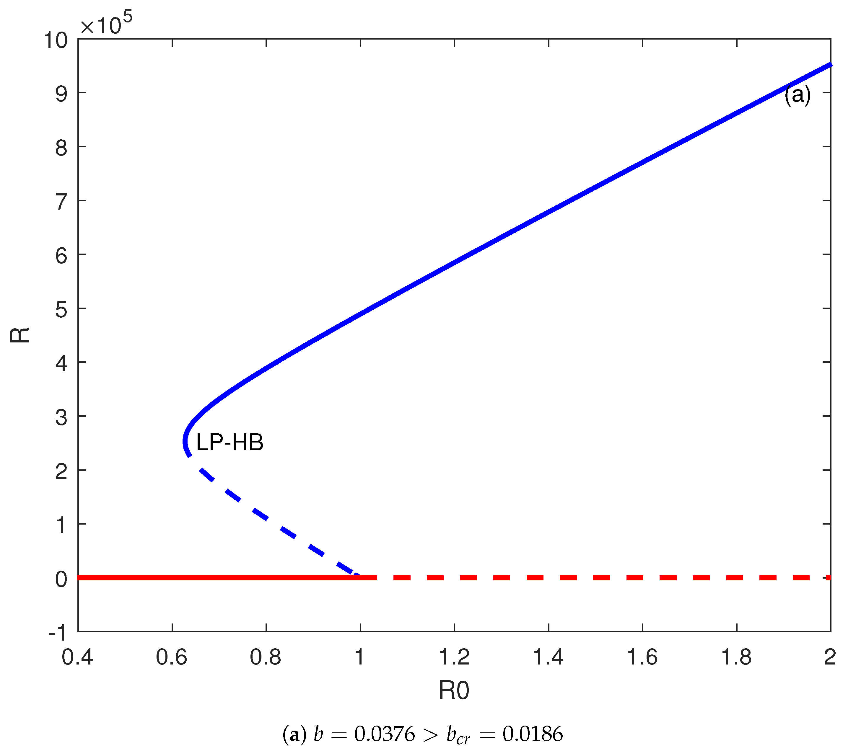
Figure 3a illustrates the bifurcation behavior for $b=0.0376$, which is the actual fitted value and which is larger than the critical value. On the diagram, the occurrence of a static limit point is at ${\mathcal{R}}_0=0.62721$, and a Hopf point is at $R_0=0.62722$. The limit point and Hopf point are very close to each other. Normally (not shown in the figure), an unstable periodic branch would bifurcate from the subcritical Hopf point and collide homoclinically with the static branch. However, the details are too small to have a practical impact given the closeness of the Hopf and limit points.

It can be concluded from the diagram that the disease-free solution coexists with the stable endemic solution for ${\mathcal{R}}_0$ extending from HB $(R_0=0.62722)$ to $({\mathcal{R}}_0=1)$. This diagram shows how important the role the parameter b of the treatment function is in controlling the disease (b accounts for the infected individuals when their treatment is delayed). For values of b larger than the critical value, the eradication of the disease does not happen when the reproduction number is reduced below one, rather it is necessary to reduce it to values below the ${\mathcal{R}}_0$ value corresponding to the Hopf point.

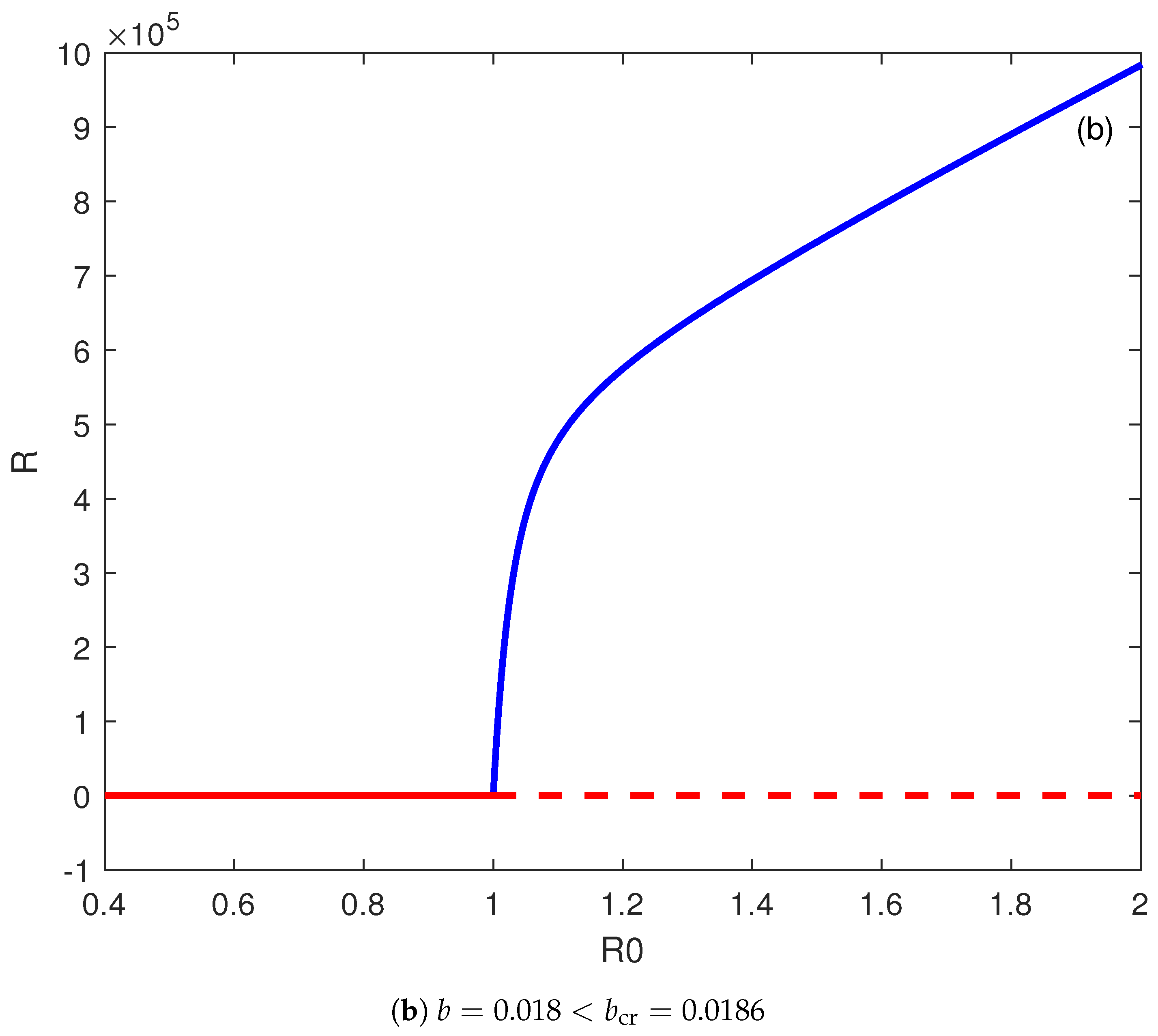
Figure 3b shows the bifurcation behavior when b is chosen smaller than the critical value, i.e., $b=0.018$. The backward bifurcation no longer exists and, instead, there is the appearance of a forward bifurcation, and the disease-free equilibrium is the only stable solution for ${\mathcal{R}}_0<1$. The disease can be suppressed if the basic reproduction number falls below the value of one.

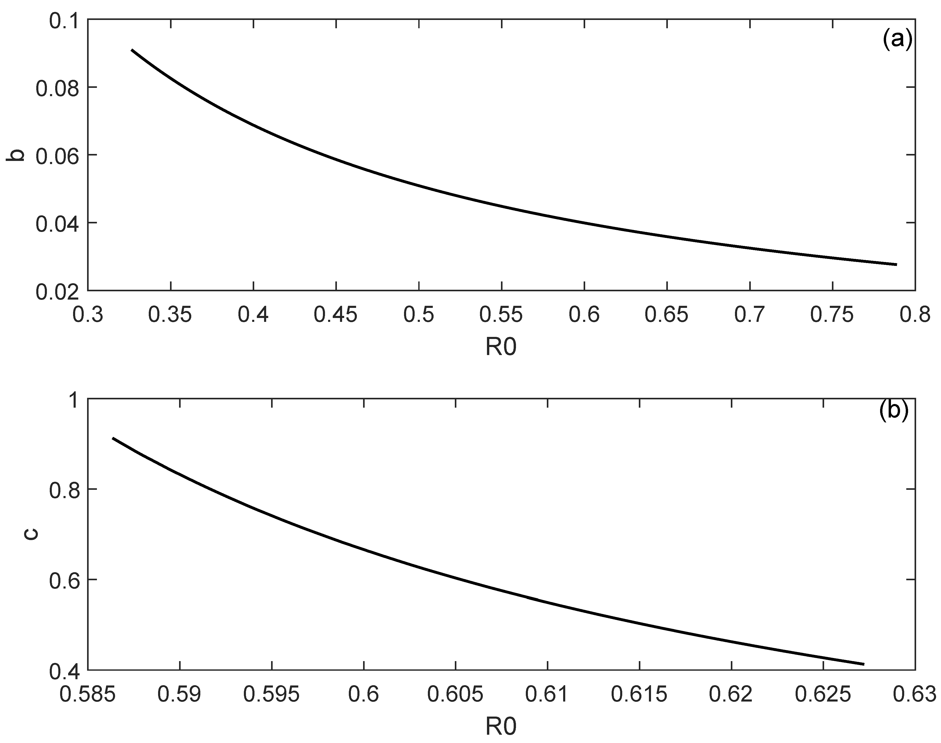
Next, we show how the model parameters affect the range of the backward bifurcation. This can be illustrated by showing the locus of the Hopf point as a function of the selected model parameters. Our numerical simulations showed that, other than b and c, which are the parameters associated with the treatment function, the change in the locus of the Hopf point was very small even when the values of model parameters were changed over a wide range.

The effects of b and c on the locus of the Hopf point are shown in Figure 4. It can be observed that a decrease of either b and c would increase the value of ${\mathcal{R}}_0$ at which the Hopf point occurs, and this would reduce the range of the backward bifurcation since the Hopf point would occur at large values of $R_0$.

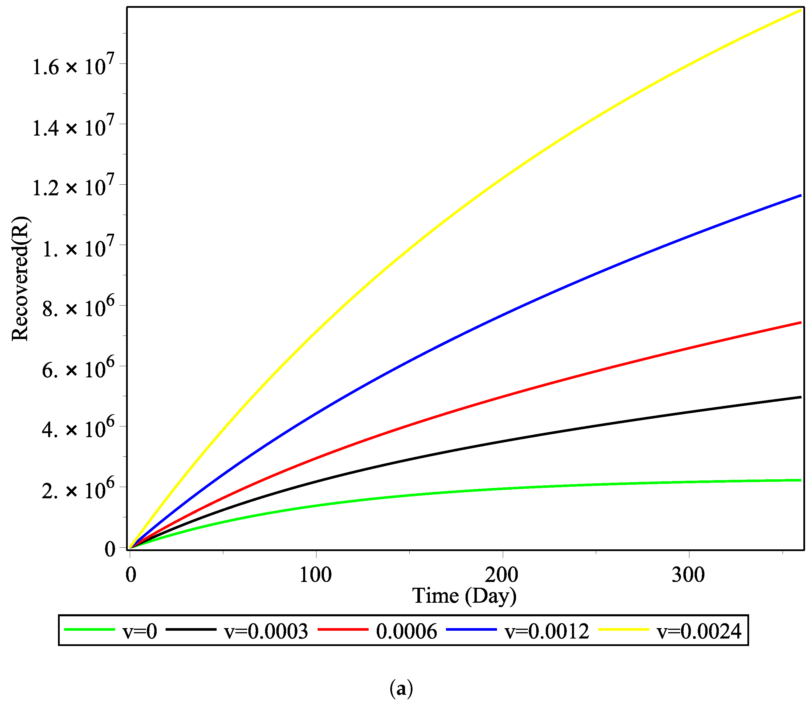
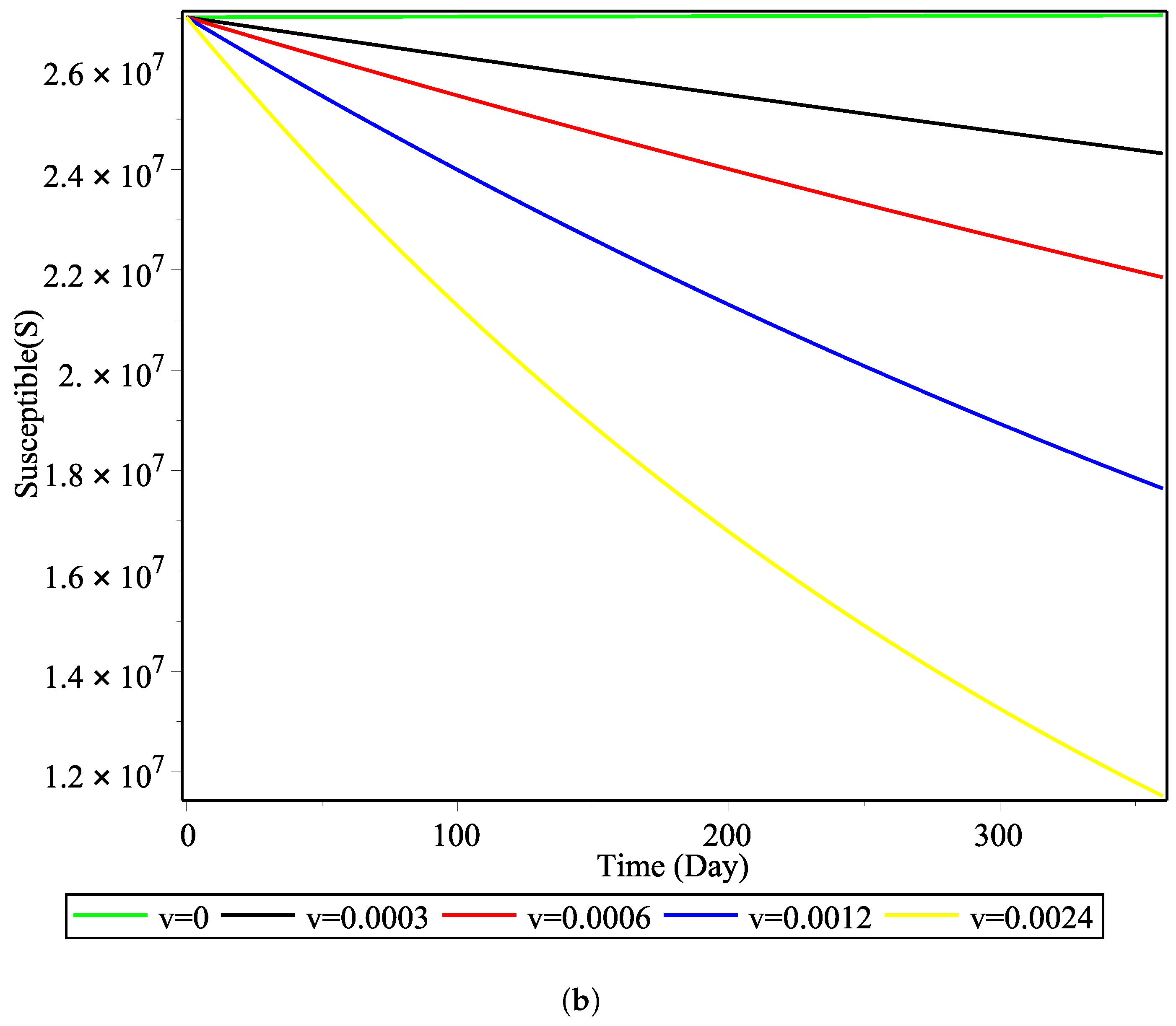
The vaccination rate does not greatly affect the backward bifurcation, but it does affect the time evolution of the disease. Figure 5 shows the effect of the vaccination rate v taking the values of $0,0.0003,0.0006,0.0012$ to $0.0024$. It can be observed that, in the window of one year, the effect of doubling the vaccination rate each year has a highly nonlinear effect on the number of susceptible and recovered individuals. This shows that the giving of vaccines to the susceptible group is influential in increasing the total population of recovered COVID-19 patients. These results are pertinent to the vaccination rate and in line with previous work carried out in Indonesia using a simpler model that did not consider a treatment function [10].

6. Conclusions

This paper studied the dynamical behavior of a SEIR model for the propagation of COVID-19. The model included a constant vaccination rate and a nonlinear treatment function in addition to a saturated incidence rate. The dynamics of the model were analyzed, and the basic reproduction number was derived. The model was fitted to the COVID-19 data of Saudi Arabia.

The main behavior found in the model was Hopf and backward bifurcations. The analysis also showed that the capacity of the treatment and the saturation factor measuring the effect of the infected individual, when delayed for treatment, played important roles in the existence of backward bifurcation. The remaining model parameters, including the vaccination rate, had a minimal effect on the occurrence of backward bifurcation. The vaccination rate, on the other hand, had an important effect on the time evolution of the disease.

References

- He, S.; Peng, Y.; Sun, K. SEIR modeling of the Covid-19 and its dynamics. Nonlinear Dyn. 2020, 101, 1–14. [Google Scholar] [CrossRef] [PubMed]
- Ajbar, A.; Alqahtani, R.; Boumaza, M. Dynamics of an SIR Based COVID 19 model with linear incidence rate, nonlinear removal rate, and public awareness. Front. Phys. 2021, 9, 13. [Google Scholar] [CrossRef]
- Sardar, T.; Nadim, S.; Rana, S.; Chattopadhyay, J. Assessment of lockdown effect in some states and overall India: A predictive mathematical study on COVID-19 outbreak. Chaos Soliton. Fract. 2020, 139, 110078. [Google Scholar] [CrossRef]
- Silva, C.J.; Cruz, C.; Torres, D.F.; Muñuzuri, A.P.; Carballosa, A.; Area, I.; Nieto, J.J.; Fonseca-Pinto, R.; Passadouro, R.; Dos Santos, E.S.; et al. Optimal control of the COVID-19 pandemic: Controlled sanitary deconfinement in Portugal. Sci. Rep. 2021, 11, 3451. [Google Scholar] [CrossRef]
- Mwalili, S.; Kimathi, M.; Ojiambo, V.; Gathungu, D.; Mbogo, R. SEIR model for Covid-19 dynamics incorporating the environment and social distancing. BMC Res. Notes 2020, 13, 352. [Google Scholar] [CrossRef] [PubMed]
- Linka, K.; Peirlinck, M.; Costabal, F.S.; Kuhl, E. Outbreak dynamics of COVID-19 in Europe and the effect of travel restrictions. Comput. Methods Biomech. Biomed. Eng. 2020, 23, 710–717. [Google Scholar] [CrossRef]
- Feng, L.X.; Jing, S.L.; Hu, S.K.; Wang, D.F. Modelling the effects of media coverage and quarantine on the COVID-19 infections in the UK. Math. Biosci. Eng. 2020, 17, 3618–3636. [Google Scholar] [CrossRef] [PubMed]
- Sarkar, K.; Khajanchi, S.; Nieto, J.J. Modeling and forecasting the COVID-19 pandemic in India. Chaos Soliton. Fract. 2020, 139, 110049. [Google Scholar] [CrossRef]
- Ndairou, F.; Area, I.; Nieto, J.J.; Silva, C.J.; Torres, D.F.M. Fractional model of COVID-19 applied to Galicia, Spain and Portugal. Chaos Soliton. Fract. 2021, 144, 110652. [Google Scholar] [CrossRef]
- Annas, S.; Pratama, M.I.; Rifandi, M.; Sanusi, W.; Side, S. Stability analysis and numerical simulation of SEIR model for pandemic Covid-19 spread in Indonesia. Chaos Soliton. Fract. 2020, 139, 110072. [Google Scholar] [CrossRef]
- Cot, C.; Cacciapaglia, G.; Islind, A.S.; Óskarsdóttir, M.; Sannino, F. Impact of US vaccination strategy on COVID-19 wave dynamics. Sci. Rep. 2021, 11, 10960. [Google Scholar] [CrossRef]
- Wintachai, P.; Prathom, K. Stability analysis of SEIR model related to efficiency of vaccines for COVID-19 situation. Heliyon 2021, 7, e06812. [Google Scholar] [CrossRef]
- Wang, W.; Ruan, S. Bifurcations in an epidemic model with constant removal rate of incentives. J. Math. Anal. Appl. 2004, 291, 775–793. [Google Scholar] [CrossRef] [Green Version]
- Wang, W. Backward Bifurcation of an Epidemic Model with Treatment. Math. Biosci. 2006, 201, 58–71. [Google Scholar] [CrossRef] [PubMed]
- Zhou, L.; Fan, M. Dynamics of an SIR Model with Limited Medical Resources Revisited. Nonlinear Anal. Real World Appl. 2012, 13, 312–324. [Google Scholar] [CrossRef]
- Zhang, J.; Jia, J.; Song, X. Analysis of an SEIR Epidemic Model with Saturated Incidence and Saturated Treatment. Funct. Sci. World J. 2014, 2014, 1–11. [Google Scholar]
- Zhang, X.; Liu, X. Backward bifurcation of an epidemic model with saturated treatment. J. Math. Anal. Appl. 2008, 348, 433–443. [Google Scholar] [CrossRef] [Green Version]
- Rehman, M.; Tauseef, I.; Aalia, B.; Shah, S.H.; Junaid, M.; Haleem, K.S. Therapeutic and vaccine strategies against Sars-CoV-2: Past, present and future. Future Virol. 2020, 15, 471–482. [Google Scholar] [CrossRef]
- Liu, X.; Liu, C.; Liu, G.; Luo, W.; Xia, N. Covid-19: Progress in diagnostics, therapy and vaccination. Theranostics 2020, 10, 7821. [Google Scholar] [CrossRef]
- Libotte, G.B.; Lobato, F.S.; Neto, A.J.S.; Platt, G.M. Determination of an optimal control strategy for vaccine administration in Covid-19 pandemic treatment. Comput. Methods Programs Biomed. 2020, 196, 105664. [Google Scholar] [CrossRef] [PubMed]
- David, A.; Oluyori, H.; Adebayo, P. Global Analysis of an SEIRS Model for COVID-19 Capturing Saturated Incidence with Treatment Response. medRxiv bioRxiv 2020. [Google Scholar] [CrossRef]
- Deng, J.; Tang, S.; Shu, H. Joint impacts of media, vaccination and treatment on an epidemic Filippov model with application to COVID-19. J. Theor. Biol. 2021, 523, 110698. [Google Scholar] [CrossRef]
- Zhang, T.; Kang, R.; Wang, K.; Liu, J. Global dynamics of an SEIR epidemic model with discontinuous treatment. Adv. Differ. Equ. 2015, 2015, 361. [Google Scholar] [CrossRef] [Green Version]
- Corduneanu, C. Principles of Differential and Integral Equations; Allyn and Bacon: Boston, MA, USA, 1971. [Google Scholar]
- Van den Driessche, P.; Watmough, J. Reproduction numbers and subthreshold endemic equilibria for compartmental models of disease transmission. Math. Biosci. 2002, 180, 29–48. [Google Scholar] [CrossRef]
- Castillo-Chavez, C.; Song, B. Dynamical models of tuberculosis and their applications. Math. Biosci. Eng. 2004, 1, 361–404. [Google Scholar] [CrossRef]
- Saudi Ministry of Health. Available online: https://www.moh.gov.sa/en/Pages/Default.aspx (accessed on 2 November 2020).
- General Authority for Statistics, Saudi Arabia. Available online: https://www.stats.gov.sa/en/5305; https://covid19.moh.gov.sa/; (accessed on 2 November 2020).
- Doedel, E.J.; Kernevez, J.P. Auto: Software for Continuation and Bifurcation Problems in Ordinary Differential Equations; CIT Press: Pasadena, CA, USA, 1986. [Google Scholar]
Figure 1.
Block diagram of the model. The arrows show progression from one compartment to the next.
Figure 2.
Validation of the model using COVID-19 data in Saudi Arabia for a period of 180 days starting from 24 March 2021. Red line (actual data); Blue solid line (model predictions). (a) Infected cases; (b) Recovered cases.
Figure 3.
(a) Backward bifurcation. (b) Forward bifurcation. Solid line (stable branch); dashed line (unstable branch); LP (static limit point); HB (Hopf point); blue line (endemic equilibrium); and red line (disease free equilibrium).
Figure 4.
Effect of the model parameters on the location of the Hopf point. (a) Effect of saturation factor (b); (b) Effect of maximal supplied medical resources (c).
Figure 5.
Effect of vaccination rate on the number of: (a) recovered cases and (b) susceptible cases.
Publisher’s Note: MDPI stays neutral with regard to jurisdictional claims in published maps and institutional affiliations. |
© 2021 by the authors. Licensee MDPI, Basel, Switzerland. This article is an open access article distributed under the terms and conditions of the Creative Commons Attribution (CC BY) license (https://creativecommons.org/licenses/by/4.0/).
Share and Cite
MDPI and ACS Style
Alqahtani, R.T.; Ajbar, A. Study of Dynamics of a COVID-19 Model for Saudi Arabia with Vaccination Rate, Saturated Treatment Function and Saturated Incidence Rate. Mathematics 2021, 9, 3134. https://doi.org/10.3390/math9233134
AMA Style
Alqahtani RT, Ajbar A. Study of Dynamics of a COVID-19 Model for Saudi Arabia with Vaccination Rate, Saturated Treatment Function and Saturated Incidence Rate. Mathematics. 2021; 9(23):3134. https://doi.org/10.3390/math9233134
Chicago/Turabian StyleAlqahtani, Rubayyi T., and Abdelhamid Ajbar. 2021. "Study of Dynamics of a COVID-19 Model for Saudi Arabia with Vaccination Rate, Saturated Treatment Function and Saturated Incidence Rate" Mathematics 9, no. 23: 3134. https://doi.org/10.3390/math9233134
Note that from the first issue of 2016, this journal uses article numbers instead of page numbers. See further details here.