

A New Polymorphic Comprehensive Model for COVID-19 Transition Cycle Dynamics with Extended Feed Streams to Symptomatic and Asymptomatic Infections

Abstract
:1. Introduction
2. Brief History of COVID-19 Mutants
3. Comprehensive SEIR (PCom–SEIR) Model Definition
- (1)
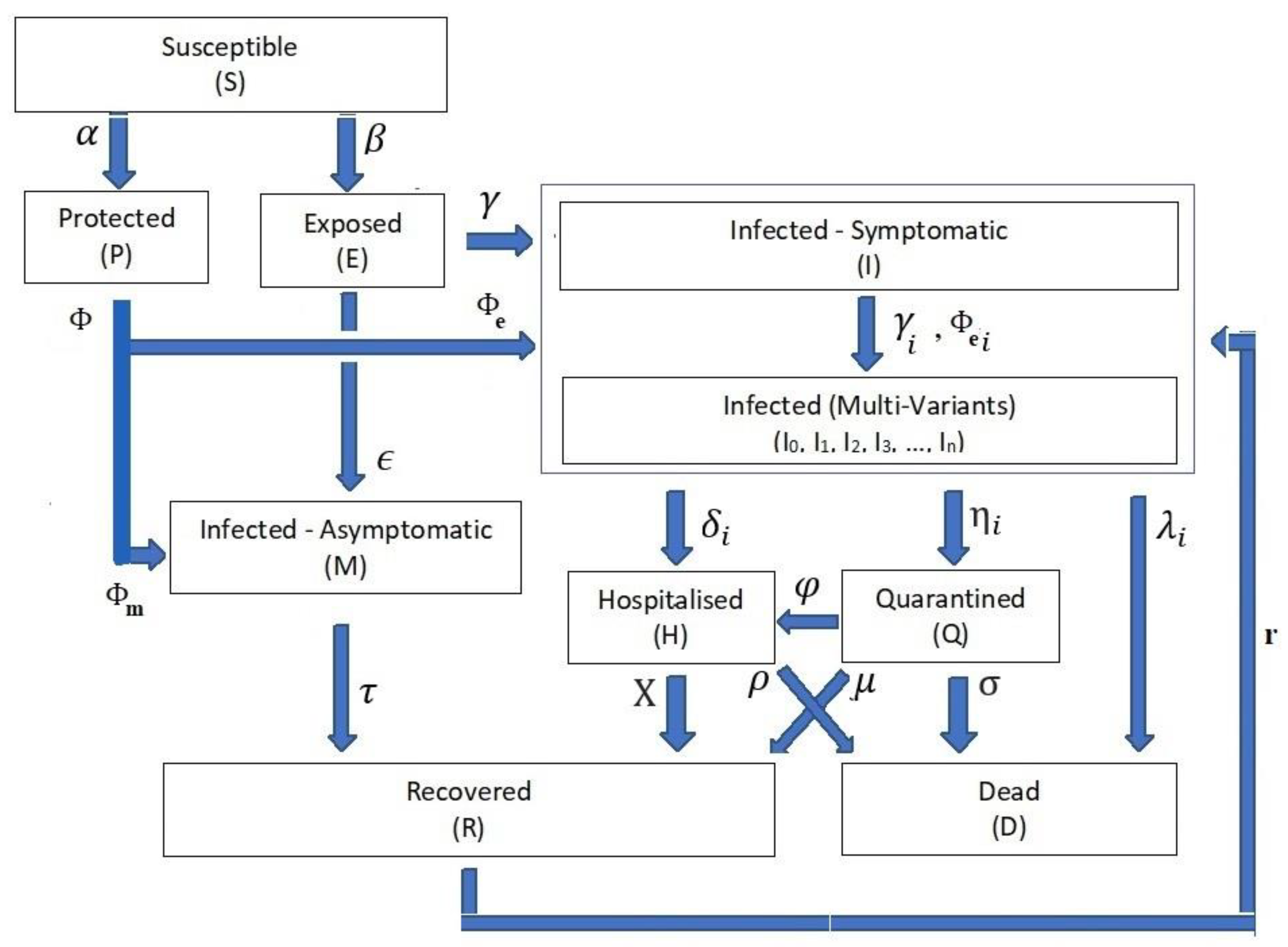
- The infection stage’s population time-dependent variable is Z(t), where the Z(t) ∈ {S(t), P(t), E(t), I(t), Ii(t), M(t), H(t), Q(t), D(t), R(t)}. Table 1 shows the definitions of these time-dependent variables. For the rest of the paper, we drop the time-independent notation for stage rate variables to ease reading except when necessary.
- (2)
- (3)
- i ∈ {0, 1, 2, …, n}, where n is defined as the total number of variants, including the mainstream I0(t).

| Variable (Z(t)) | Description | |
|---|---|---|
| 1 | S(t) | The population of the susceptible stage. |
| 2 | P(t) | The population of the protected stage. |
| 3 | E(t) | The population for the exposed stage. |
| 4 | I(t) | The infection population of the symptomatic infection stage. |
| 5 | Ii(t), i ∈ {0, 1, 2,…, n} | The population of the ith symptomatic infection variant. |
| 6 | M(t) | The population of the asymptomatic infection. |
| 7 | Q(t) | The population of the quarantined stage. |
| 8 | H(t) | The population of the hospitalisation stage. |
| 9 | D(t) | The population of the death stage. |
| 10 | N | Country’s population. |
| Parameter (ψ) | Feeding Parameter | ||
|---|---|---|---|
| From Stage | To Stage | ||
| 1 | α | Susceptible (S) | Protected (P) |
| 2 | Β | Exposed (E) | |
| 3 | Φ | Protected (P) | |
| 4 | Φe | Protected Pe = P ∗ Φe component | Symptomatic infection (I) |
| 5 | Φm | Protected Pm = P ∗ Φm component | Asymptomatic infection (M) |
| 6 | ϒ | Exposed (E) | Symptomatic infection (I) |
| 7 | ϵ | Asymptomatic infection (M) | |
| 8 | Ii | Symptomatic infection (I) | Symptomatic infection variant i |
| 9 | ϒi | Exposed component | Symptomatic infection variant (Ii) |
| 10 | Φei | Protected component | |
| 11 | Δi | Symptomatic variant with (Ii) | Hospitalisation (H) |
| 12 | ηi | Quarantine (Q) | |
| 13 | λi | Death (D) | |
| 14 | Τ | Asymptomatic (M) | Recovered (R) |
| 15 | Χ | Hospitalisation (H) | Recovered (R) |
| 16 | Ρ | Death (D) | |
| 17 | Μ | Quarantine (Q) | Recovered (R) |
| 18 | Σ | Death (D) | |
| 19 | Φ | Hospitalisation (H) | |
| 20 | ri | Recovered component | Symptomatic infection variant i |
- (A)
- Differential Equation System: The relationships from Equations (1)–(10) form the structure of the differential equation set that governs the dynamics of the transitions between the COVID-19 life cycle stages (Figure 1).
- (B)
- Stage Population Transition:
- (C)
- Extended Feed Streams:
- (D)
- Infection Categories:
- (E)
- Health Efforts: It is vitally important to point out that the infection stage’s population Z and the cumulative influencing probability parameter ψ on the infection life cycle govern the transitions’ influx and outflux, as shown in Figure 1. The controlling efforts regulated and imposed by the health authorities are typically the most dominant element within the cumulative parameter due to the state-wide law support. The PCom–SEIR model’s equation parameters map those factors across all stages. Additionally, each of these parameters is a random variable along the time axis. Consequently, the PCom–SEIR model simulates the convoluted impact of the manipulating efforts on each stage population Z. Indeed, this was the basis of the convolution model (CPM) proposed in [13]. Hence, we can write the following:
- (F)
- I.
- symptomatic infection variants ;
- II.
- Q.
- I.
- Symptomatic infection variants .
- I.
- symptomatic infection variants ;
- II.
- H;
- III.
- Q.
- I.
- H;
- II.
- Q;
- III.
- M.
- (G)
- Equations’ Constraints:
- I.
- Equation (10) indicates the governing constraints that ensure the equilibrium between the in and out stage populations within the COVID-19 infection cycle defined from Equations (3)–(9). Equation (10) reflects the fact that all symptomatic infection data I(t) include all variant types without any variant-specific information. This means we could not use published COVID-19 data to verify the derived model. Hence, we needed to use a different approach to validate the derived model, as explained in Section 4.
- II.
- In Equation (10b), reflects the fact that the effective growth rates Ii(t) of each variant are independent of each other, so there is no guarantee they will have the same rate on a given day. Additionally, this Equation is necessary to ensure the conservation of the total population N. However, there is no well-defined data-based knowledge about the level of impedance of multi-variant infection to vaccination.
4. PCom–SEIR Model Computation
4.1. The Country Use Cases
4.2. The Initial Condition Use Cases
4.3. Vaccination Representation Use Cases
4.4. The Date Range Use Cases
4.5. Implementation Steps
5. Results and Discussion
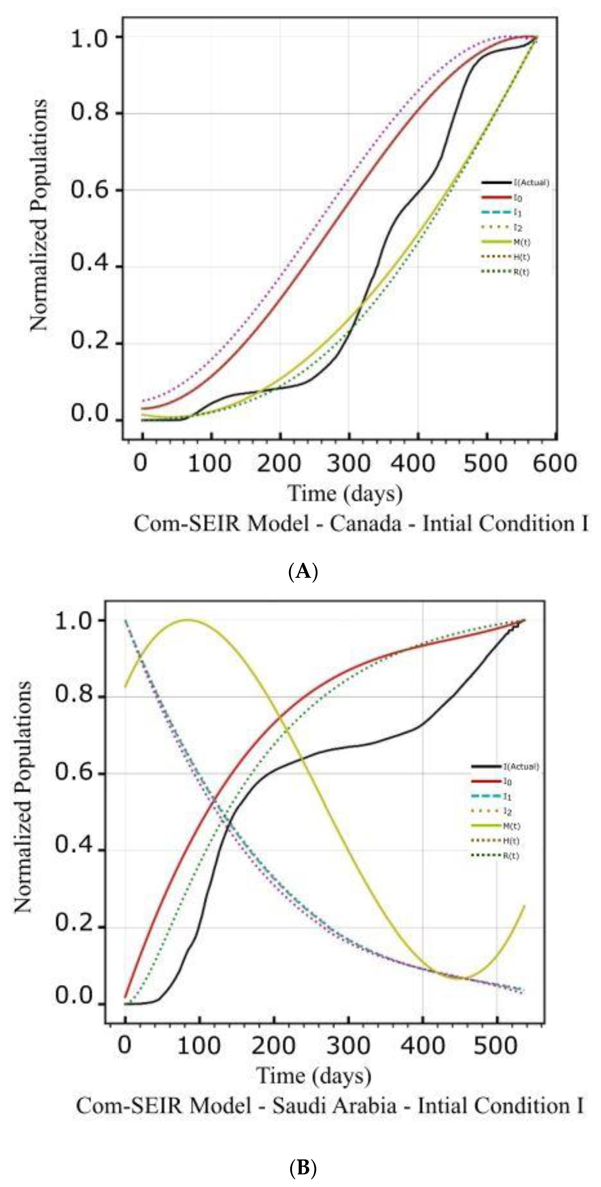
5.1. PCom–SEIR Model and 30-Day Prediction for Canada
5.1.1. Initial Conditions I—Canada
5.1.2. Initial Conditions II—Canada
5.2. PCom–SEIR Model and 30-Day Prediction for Saudi Arabia
5.2.1. Initial Conditions I—Saudi Arabia
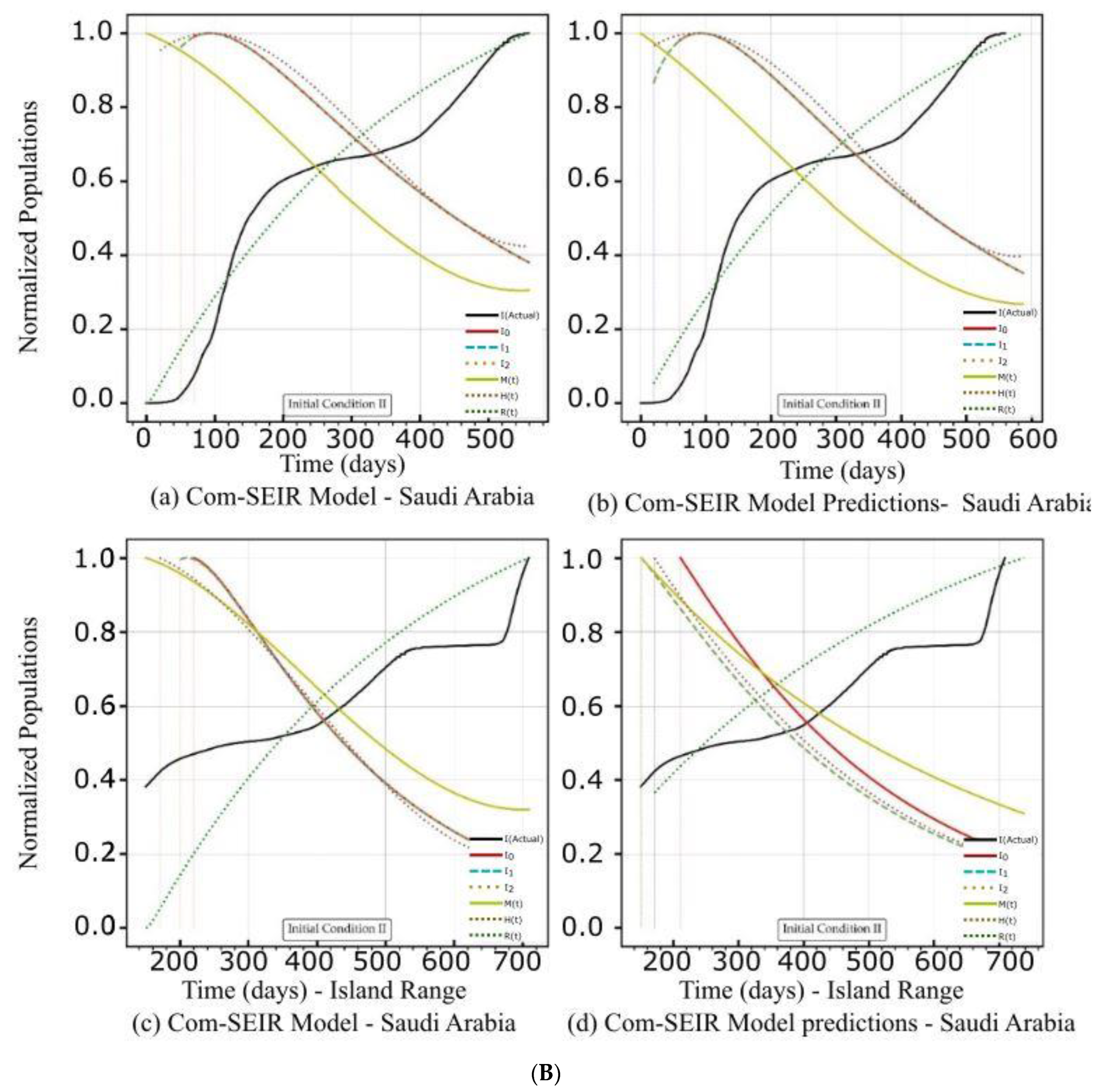
5.2.2. Initial Conditions II—Saudi Arabia
6. Conclusions
6.1. Validity and Reliability Use Cases
6.2. Model Generality
6.3. Future Work—Hybrid Approach
Author Contributions
Funding
Data Availability Statement
Acknowledgments
Conflicts of Interest
References
- Lv, L.; Li, G.; Chen, J.; Liang, X.; Li, Y. Comparative genomic analysis revealed specific mutation pattern between human coronavirus SARS-CoV-2 and Bat-SARSr-CoV RaTG13. BioRxiv 2020. [Google Scholar] [CrossRef]
- Balabdaoui, F.; Mohr, D. Age-stratified discrete compartment model of the COVID-19 epidemic with application to Switzerland. Sci. Rep. 2020, 10, 21306. [Google Scholar] [CrossRef] [PubMed]
- Giordano, G.; Blanchini, F.; Bruno, R.; Colaneri, P.; Di Filippo, A.; Di Matteo, A.; Colaneri, M. Modelling the COVID-19 epidemic and implementation of population-wide interventions in Italy. Nat. Med. 2020, 26, 855–860. [Google Scholar] [CrossRef]
- Godio, A.; Pace, F.; Vergnano, A. SEIR Modeling of the Italian Epidemic of SARS-CoV-2 Using Computational Swarm Intelligence. Int. J. Environ. Res. Public Health 2020, 17, 3535. [Google Scholar] [CrossRef] [PubMed]
- Shaikh, A.S.; Shaikh, I.N.; Nisar, K.S. A Mathematical Model of COVID-19 Using Fractional Derivative: Outbreak in India with Dynamics of Transmission and Control. Adv. Differ. Equ. 2020, 2020, 373. [Google Scholar] [CrossRef]
- Lin, Q.; Zhao, S.; Gao, D.; Lou, Y.; Yang, S.; Musa, S.S.; Wang, M.H.; Cai, Y.; Wang, W.; Yang, L.; et al. A conceptual model for the coronavirus disease 2019 (COVID-19) outbreak in Wuhan, China with individual reaction and governmental action. Int. J. Infect. Dis. 2020, 93, 211–216. [Google Scholar] [CrossRef]
- Roques, L.; Klein, E.K.; Papaix, J.; Sar, A.; Soubeyrand, S. Using Early Data to Estimate the Actual Infection Fatality Ratio from COVID-19 in France. Biology 2020, 9, 97. [Google Scholar] [CrossRef]
- Bakhta, A.; Boiveau, T.; Maday, Y.; Mula, O. Epidemiological Forecasting with Model Reduction of Compartmental Models. Application to the COVID-19 Pandemic. Biology 2021, 10, 22. [Google Scholar] [CrossRef]
- Mokhtari, A.; Mineo, C.; Kriseman, J.; Kremer, P.; Neal, L.; Larson, J. A multi method approach to modeling COVID 19 disease dynamics in the United States. Sci. Rep. 2021, 11, 12426. [Google Scholar] [CrossRef]
- Xie, G. A novel Monte Carlo simulation procedure for modelling COVID-19 spread over time. Sci. Rep. 2020, 10, 13120. [Google Scholar] [CrossRef]
- Sartorius, B.; Lawson, A.B.; Pullan, R.L. Modelling and predicting the spatiotemporal spread of COVID-19, associated deaths and impact of key risk factors in England. Sci. Rep. 2021, 11, 5378. [Google Scholar] [CrossRef]
- Mishra, S.; Scott, J.A.; Laydon, D.J.; Flaxman, S.; Gandy, A.; Mellan, T.A.; Unwin, H.J.T.; Vollmer, M.; Coupland, H.; Ratmann, O.; et al. Comparing the responses of the UK, Sweden, and Denmark to COVID 19 using counterfactual modelling. Sci. Rep. 2021, 11, 16342. [Google Scholar] [CrossRef] [PubMed]
- Al-Hadeethi, Y.; Ramley, I.F.E.; Sayyed, M.I. Convolution model for COVID-19 rate predictions and health effort levels computation for Saudi Arabia, France, and Canada. Sci. Rep. 2021, 11, 22664. [Google Scholar] [CrossRef] [PubMed]
- Bastos, S.B.; Cajueiro, D.O. Modeling and forecasting the early evolution of the COVID-19 pandemic in Brazil. Sci. Rep. 2020, 10, 19457. [Google Scholar] [CrossRef]
- Liu, M.; Thomadsen, R.; Yao, S. Forecasting the spread of COVID-19 under different reopening strategies. Sci. Rep. 2020, 10, 20367. [Google Scholar] [CrossRef] [PubMed]
- Zhang, Y.; You, C.; Cai, Z.; Sun, J.; Hu, W.; Zhou, X.H. Prediction of the COVID-19 outbreak in China based on a new stochastic dynamic model. Sci. Rep. 2020, 10, 21522. [Google Scholar] [CrossRef]
- Ma, R.; Zheng, X.; Wang, P.; Liu, H.; Zhang, C. The prediction and analysis of COVID-19 epidemic trend by combining LSTM and Markov method. Sci. Rep. 2021, 11, 17421. [Google Scholar] [CrossRef]
- Oraby, T.; Tyshenko, M.G.; Maldonado, J.C.; Vatcheva, K.; Elsaadany, S.; Alali, W.Q.; Longenecker, J.C.; Al-Zoughool, M. Modeling the effect of lockdown timing as a COVID-19 control measure in countries with differing social contacts. Sci. Rep. 2021, 11, 3354. [Google Scholar] [CrossRef]
- GitHub. Available online: https://raw.githubusercontent.com/datasets/covid-19/master/data/countries-aggregated.csv (accessed on 22 September 2021).
- WHO. Available online: https://www.who.int/news-room/fact-sheets/detail/middle-east-respiratory-syndrome-coronavirus-(mers-cov) (accessed on 28 October 2021).
- Gorbalenya, A.E.; Baker, S.C.; Baric, R.S.; de Groot, R.J.; Drosten, C.; Gulyaeva, A.A.; Haagmans, B.L.; Lauber, C.; Leontovich, A.M.; Neuman, B.W.; et al. The species Severe acute respiratory syndrome-related coronavirus: Classifying 2019-nCoV and naming it SARS-CoV-2. Nat. Microbiol. 2020, 5, 536. [Google Scholar]
- Na, W.; Moon, H.; Song, D. A comprehensive review of SARS-CoV-2 genetic mutations and lessons from animal coronavirus recombination in one health perspective. J. Microbiol. 2021, 59, 332–340. [Google Scholar] [CrossRef]
- Ahn, D.G.; Shin, H.J.; Kim, M.H.; Lee, S.; Kim, H.S.; Myoung, J.; Kim, B.T.; Kim, S.J. Current status of epidemiology, diagnosis, therapeutics, and vaccines for novel coronavirus disease 2019 (COVID-19). J. Microbiol. Biotechnol. 2020, 30, 313–324. [Google Scholar] [CrossRef]
- Tu, Y.F.; Chien, C.S.; Yarmishyn, A.A.; Lin, Y.Y.; Luo, Y.H.; Lin, Y.T.; Lai, W.Y.; Yang, D.M.; Chou, S.J.; Yang, Y.P.; et al. A review of SARS-CoV-2 and the ongoing clinical trials. Int. J. Mol. Sci. 2020, 21, 2657. [Google Scholar] [CrossRef] [Green Version]
- Wu, Z.; McGoogan, J.M. Characteristics of and important lessons from the coronavirus disease 2019 (COVID-19) outbreak in China: Summary of a report of 72 314 cases from the Chinese Center for Disease Control and Prevention. JAMA 2020, 323, 1239–1242. [Google Scholar] [CrossRef]
- Huang, N.E.; Qiao, F. A data-driven time-dependent transmission rate for tracking an epidemic: A case study of 2019-nCoV. Sci. Bull. 2020, 65, 425. [Google Scholar] [CrossRef] [PubMed]
- Available online: https://www.worldometers.info/coronavirus/#countries (accessed on 5 October 2021).
- Available online: https://www.who.int/en/activities/tracking-SARS-CoV-2-variants (accessed on 2 October 2021).
- Shen, X.; Tang, H.; McDanal, C.; Wagh, K.; Fischer, W.; Theiler, J.; Yoon, H.; Li, D.; Haynes, B.F.; Sanders, K.O.; et al. SARS-CoV-2 variant B. 1.1. 7 is susceptible to neutralising antibodies elicited by ancestral spike vaccines. Cell Host Microbe 2021, 29, 529–539. [Google Scholar] [CrossRef]
- Altmann, D.M.; Boyton, R.J.; Beale, R. Immunity to SARS-CoV-2 variants of concern. Science 2021, 371, 1103–1104. [Google Scholar] [CrossRef] [PubMed]
- Rees-Spear, C.; Muir, L.; Griffith, S.A.; Heaney, J.; Aldon, Y.; Snitselaar, J.L.; Thomas, P.; Graham, C.; Seow, J.; Lee, N.; et al. The effect of spike mutations on SARS-CoV-2 neutralisation. Cell Rep. 2021, 34, 108890. [Google Scholar] [CrossRef] [PubMed]
- Hu, J.; Peng, P.; Wang, K.; Fang, L.; Luo, F.Y.; Jin, A.S.; Liu, B.Z.; Tang, N.; Huang, A.L. Emerging SARS-CoV-2 variants reduce neutralisation sensitivity to convalescent sera and monoclonal antibodies. Cell. Mol. Immunol. 2021, 18, 1061–1063. [Google Scholar] [CrossRef]
- Wang, P.; Nair, M.S.; Liu, L.; Iketani, S.; Luo, Y.; Guo, Y.; Wang, M.; Yu, J.; Zhang, B.; Kwong, P.D.; et al. Antibody resistance of SARS-CoV-2 variants B.1.351 and B.1.1.7. Nature 2021, 593, 130–135. [Google Scholar] [CrossRef] [PubMed]
- Moyo-Gwete, T.; Madzivhandila, M.; Makhado, Z.; Ayres, F.; Mhlanga, D.; Oosthuysen, B.; Lambson, B.E.; Kgagudi, P.; Tegally, H.; Iranzadeh, A.; et al. SARS-CoV-2 501Y. V2 (B. 1.351) elicits cross-reactive neutralising antibodies. bioRxiv 2021. preprint. [Google Scholar]
- Koyama, T.; Platt, D.; Parida, L. Variant analysis of SARS-CoV-2 genomes. Bull. World Health Organ. 2020, 98, 495. [Google Scholar] [CrossRef]
- Slavov, S.N.; Patané, J.S.; Bezerra, R.D.S.; Giovanetti, M.; Fonseca, V.; Martins, A.J.; Viala, V.L.; Rodrigues, E.S.; Santos, E.V.; Barros, C.R.; et al. Genomic monitoring unveil the early detection of the SARS-CoV-2 B. 1.351 lineage (20H/501Y. V2) in Brazil. J. Med. Virol. 2021, 93, 6782–6787. [Google Scholar] [CrossRef] [PubMed]
- Shen, X.; Tang, H.; Pajon, R.; Smith, G.; Glenn, G.M.; Shi, W.; Korber, B.; Montefiori, D.C. Neutralisation of SARS-CoV-2 Variants B.1.429 and B.1.351. N. Engl. J. Med. 2021, 384, 2352–2354. [Google Scholar] [CrossRef]
- Singh, J.; Samal, J.; Kumar, V.; Sharma, J.; Agrawal, U.; Ehtesham, N.Z.; Sundar, D.; Rahman, S.A.; Hira, S.; Hasnain, S.E. Structure-Function Analyses of New SARS-CoV-2 Variants B.1.1.7, B.1.351 and B.1.1.28.1: Clinical, Diagnostic, Therapeutic and Public Health Implications. Viruses 2021, 13, 439. [Google Scholar] [CrossRef] [PubMed]
- Gupta, R.K. Will SARS-CoV-2 variants of concern affect the promise of vaccines? Nat. Rev. Immunol. 2021, 21, 340–341. [Google Scholar] [CrossRef] [PubMed]
- Focosi, D.; Maggi, F. Neutralising antibody escape of SARS-CoV-2 spike protein: Risk assessment for antibody-based COVID-19 therapeutics and vaccines. Rev. Med. Virol. 2021, 31, e2231. [Google Scholar] [CrossRef] [PubMed]
- Fontanet, B.; Autran, B.; Lina, M.P.; Kieny, S.S.; Karim, A.; Sridhar, D. SARS-CoV-2 variants and ending the COVID-19 pandemic. Lancet 2021, 397, 952–954. [Google Scholar] [CrossRef] [PubMed]
- Campbell, F.; Archer, B.; Laurenson-Schafer, H.; Jinnai, Y.; Konings, F.; Batra, N.; Pavlin, B.; Vandemaele, K.; Van Kerkhove, M.D.; Jombart, T.; et al. Increased transmissibility and global spread of SARS-CoV-2 variants of concern as at June 2021. Eurosurveillance 2021, 26, 2100509. [Google Scholar] [CrossRef] [PubMed]
- Mohammadi, M.; Shayestehpour, M.; Mirzaei, H. The impact of spike mutated variants of SARS-CoV2 [Alpha, Beta, Gamma, Delta, and Lambda] on the efficacy of subunit recombinant vaccines. Braz. J. Infect. Dis. 2021, 25, 101606. [Google Scholar] [CrossRef]
- Hajj-Hassan, H.; Hamze, K.; Sater, F.A.; Kizilbash, N.; Khachfe, H.M. Probing the Increased Virulence of Severe Acute Respiratory Syndrome Coronavirus 2 B.1.617 (Indian Variant) From Predicted Spike Protein Structure. Cureus 2021, 13, e16905. [Google Scholar] [CrossRef]
- Romero, P.E.; Dávila-Barclay, A.; Salvatierra, G.; González, L.; Cuicapuza, D.; Solís, L.; Marcos-Carbajal, P.; Huancachoque, J.; Maturrano, L.; Tsukayama, P. The emergence of SARS-CoV-2 variant lambda (C. 37) in South America. Microbiol. Spectr. 2021, 9, e00789-21. [Google Scholar] [CrossRef]
- Tada, T.; Zhou, H.; Dcosta, B.M.; Samanovic, M.I.; Mulligan, M.J.; Landau, N.R. SARS-CoV-2 lambda variant remains susceptible to neutralisation by mRNA vaccine-elicited antibodies and convalescent serum. bioRxiv 2021. preprint. [Google Scholar]
- Acevedo, M.L.; Alonso-Palomares, L.; Bustamante, A.; Gaggero, A.; Paredes, F.; Cortés, C.P.; Valiente-Echeverría, F.; Soto-Rifo, R. Infectivity and immune escape of the new SARS-CoV-2 variant of interest Lambda. medRxiv 2021. preprint. [Google Scholar]
- Lanas, D.; Bruel, T.; Grzelak, L.; Guivel-Benhassine, F.; Staropoli, I.; Porrot, F.; Planchais, C.; Buchrieser, J.; Rajah, M.M.; Bishop, E.; et al. Sensitivity of infectious SARS-CoV-2 B.1.1.7 and B.1.351 variants to neutralising antibodies. Nat. Med. 2021, 27, 917–924. [Google Scholar] [CrossRef]
- Zhang, Y.; Yu, X.; Sun, H.; Tick, G.R.; Wei, W.; Jin, B. COVID-19 infection and recovery in various countries: Modeling the dynamics and evaluating the non-pharmaceutical mitigation scenarios. arXiv 2020, arXiv:2003.13901. [Google Scholar]
- Peng, L.; Yang, W.; Zhang, D.; Zhuge, C.; Hong, L. Epidemic analysis of COVID-19 in China by dynamical modelling. MedRxiv Epidemiol. 2020, 2002, 06563. [Google Scholar]
- Storn, P.; Price, K. A Simple and Efficient Heuristic for Global Optimisation over Continuous Spaces. J. Glob. Optim. 1997, 11, 341–359. [Google Scholar] [CrossRef]
- Python Optimization (Scipy. Optimize). Available online: https://docs.scipy.org/doc/scipy/tutorial/optimize.html (accessed on 10 October 2022).
- Lerch, F.; Ultsch, A.; Lötsch, J. Distribution Optimisation: An evolutionary algorithm to separate Gaussian mixtures. Sci. Rep. 2020, 10, 648. [Google Scholar] [CrossRef] [Green Version]
- Covões, T.F.; Hruschka, E.R.; Ghosh, J. Evolving Gaussian Mixture Models with Splitting and Merging Mutation Operators. Evol. Comput. 2015, 24, 293–317. Available online: http://www.mitpressjournals.org/doi/10.1162/EVCO_a_00152 (accessed on 1 August 2022). [CrossRef] [PubMed] [Green Version]


| Initial Condition I | |||||||
| S0 | P0 | E0 | I0 | M0 | H0 | Q0 | R0 |
| N | 0.1 * N | 0.9 * N | I[0] | M[0] | H[0] | Q[0] | R[0] |
| Initial Condition II | |||||||
| S0 | P0 | E0 | I0 | M0 | H0 | Q0 | R0 |
| N | 0.7 * N | 0.3 * N | 1.0 | 0.0 | 0.0 | 0.0 | 0.0 |
| Date Range 1 | Date Range 2 (Island Range) | |||||
|---|---|---|---|---|---|---|
| 560 Points (Days) | 23 January 2020, to 5 August 2021 | 23 April 2020, to 4 November 2021 | ||||
| Initial Conditions (ICs) | I, II | I, II | I, II | I, II | I, II | I, II |
| Context | Models and Predictions | Parameters | Convergence Ratio | Models and Predictions | Parameters | Convergence Ratio |
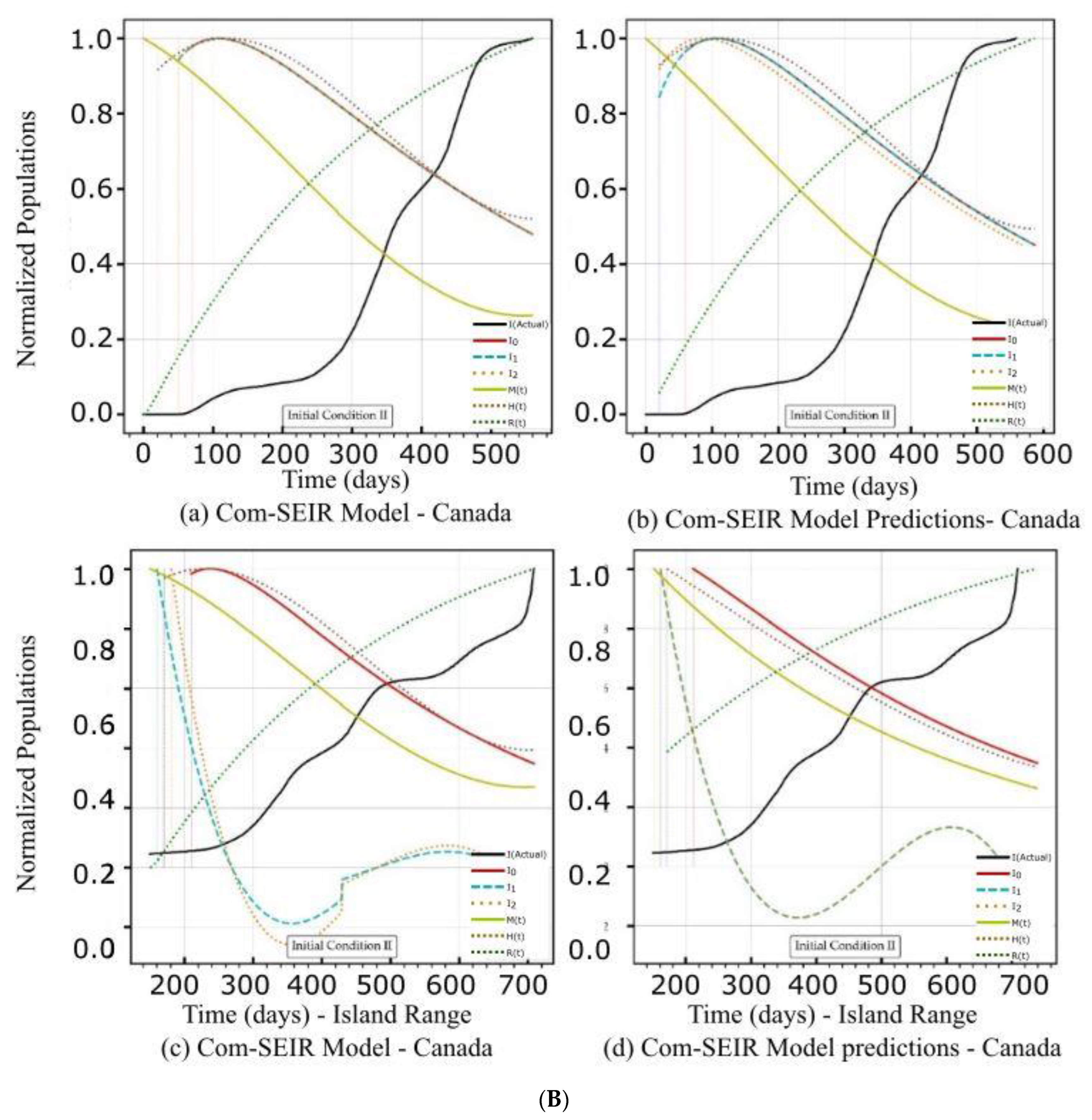
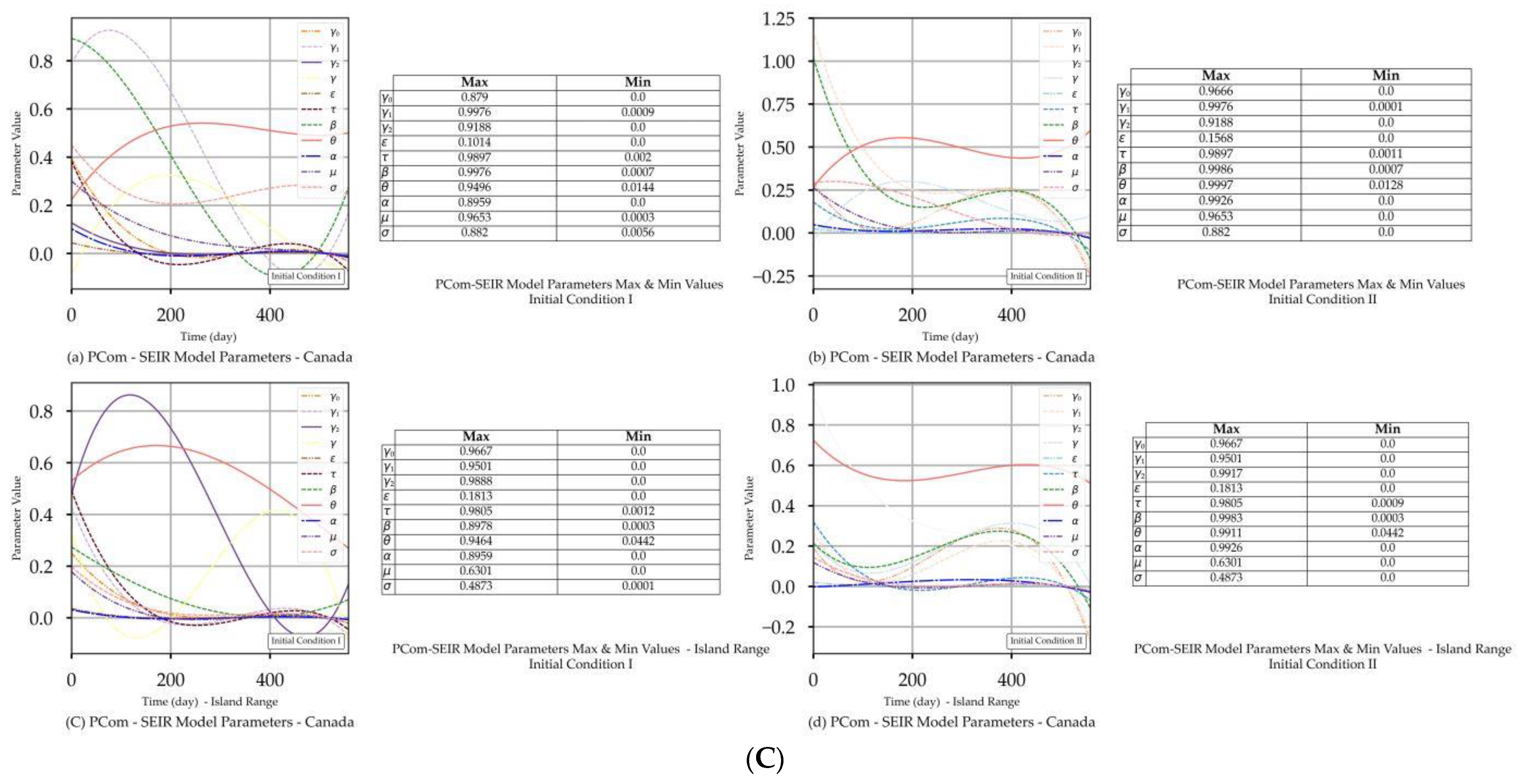
| Canada | Figure 2A(a,b) Figure 2B(a,b) | Figure 2C(a) | Figure 4a | Figure 2A(c,d) Figure 2B(c,d) | Figure 2C(d) | Figure 4a |
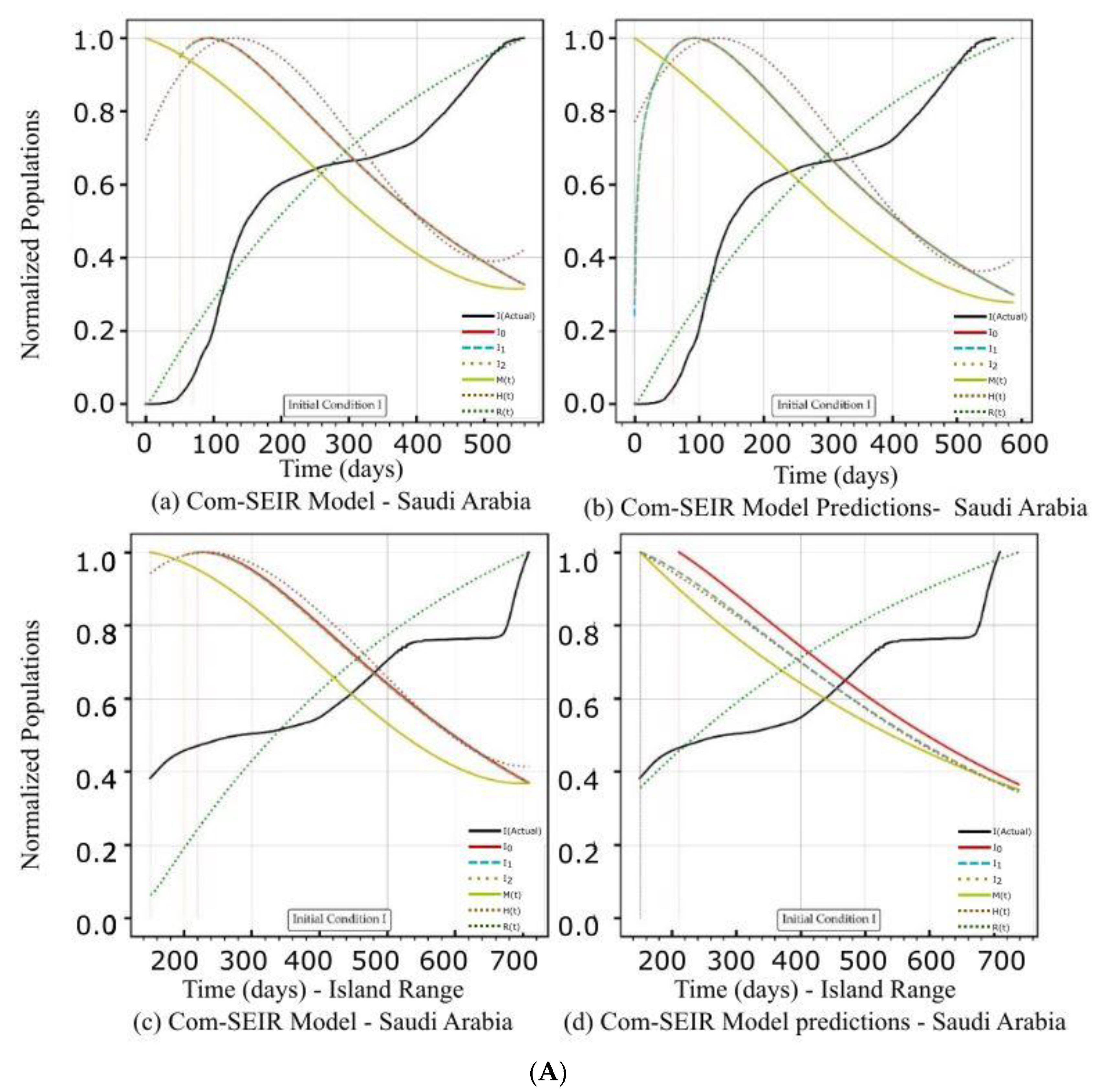
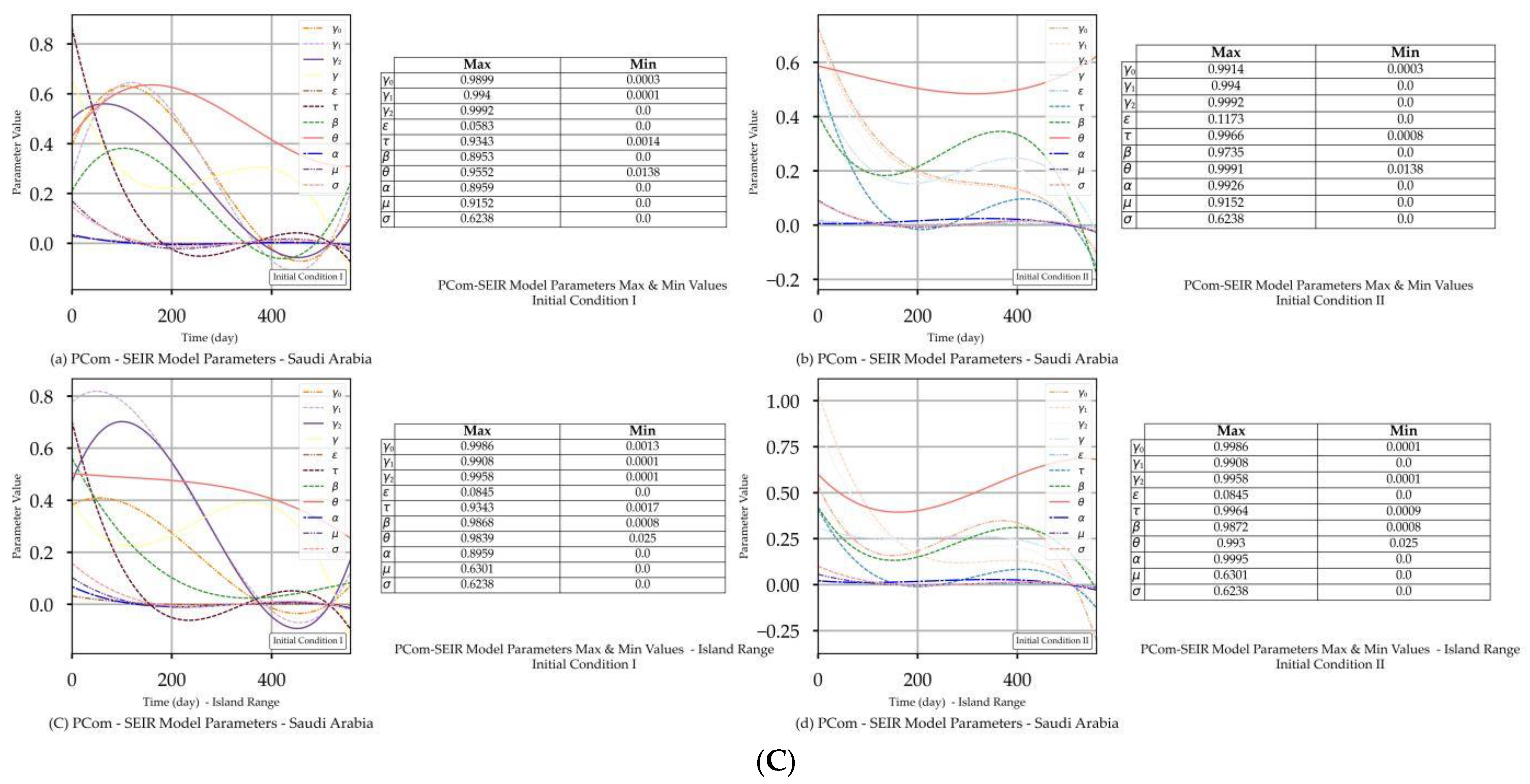
| Saudi Arabia | Figure 3A(a,b) Figure 3B(a,b) | Figure 3C(a) | Figure 4b | Figure 3A(c,d) Figure 3B(c,d) | Figure 3C(d) | Figure 4b |
| Date Range 1 (Start Date: 0 Days). | Date Range 2 (Start Date: 100 Days). | |||
|---|---|---|---|---|
| Figure | Model—Figure 2A(a) | Prediction—Figure 2A(b) | Model—Figure 2A(c) | Prediction—Figure 2A(d) |
| Curve discontinuity | Not stable over the first 50+ days. | The {Ii} curves showed an improvement, but we still needed to truncate the curve’s start by 20 points. | The prediction curves for {I1, I2} did not show discontinuity, but I0 (main stream) did. | |
| Peak position | The first peaks located before the 100 days were due to solution discontinuity. The peak on the 120th day was within the range of the actual stable solution. | The curves for {Ii} had nearly the same peak on the 200th day after the start date. | The {Ii} curves shared the same peak on the 110th day after the start date. | |
| Curve profiles | The {Ii} curves showed the same profile with a limited plateau. | The {Ii} curves showed different individual profiles but all had small plateaus. | The {Ii} curves showed the same profile with a noticeable plateau. | The {Ii} curves showed the same profile but differed from the models. |
| Decline rate | The predicted declines of the infection growth rate were relatively slower than those of the model. | The predicted infection growth rate declines were slower than those of the models. | ||
| Decline slope | 2.15/4 | 2.0/4 | 2.2/4 | 1.9/4 |
| Date Range 1 (Start Date: 0 Days). | Date Range 2 (Start Date: 100 Days). | |||
|---|---|---|---|---|
| Figure | Model—Figure 2B(a) | Prediction—Figure 2B(b) | Model—Figure 2B(c) | Prediction—Figure 2B(d) |
| Curve discontinuity | Relatively stable over the first 50 days. | The {I1, I2} curves did not show a realistic solution, but I0 (main stream) did. | ||
| Peak position | The peak appeared on the 110th day. | The peak appeared on the 100th day. | The I0 curve peaked at the 150th day (i.e., 250th day) after the start date. | The I0 curve showed no peak. |
| Curve profiles | The {Ii} curves showed the same profile with a limited plateau. | The {Ii} curves showed different individual profiles with a limited plateau. | The I0 curve showed nearly the exact profile of Date Range 1 with a finite plateau. | The I0 curve showed a different profile than the model without a plateau. |
| Decline rate | The predicted infection growth decline was at nearly the same rate as that of the model. However, it showed a steeper decline than that of IC-I. | The predicted infection growth decline rate was slower than that of the model. | ||
| Decline slope | 2.5/4 | 2.5/4 | 2.4/4 | 2.1/4 |
| Date Range 1 (Start Date: 0 Days). | Date Range 2 (Start Date: 100 Days). | |||
|---|---|---|---|---|
| Figure | Model—Figure 3A(a) | Prediction—Figure 3A(b) | Model—Figure 3A(c) | Prediction—Figure 3A(d) |
| Curve discontinuity | The {Ii} curves showed an improvement, but we still needed to truncate the curve’s start by 50 points. | The {Ii} curves showed good improvement without the need to truncate the curve’s start. | The {Ii} curves showed an improvement, but we still needed to truncate the curve’s start by 50 points. | The prediction curves for {Ii} did not show a discontinuity. |
| Peak position | The peaks appeared on the 110th day. | The peaks appeared on the 90th day. | The curves for {Ii} had nearly the same peak on the 120th day after the start date. | The {I1, I2} curves shared the same peak on the 30th day after the start date. I0 showed no peak. |
| Curve profiles | The {Ii} curves showed the same profile with a noticeable plateau. | The {Ii} curves showed the same profile with a noticeable plateau. The prediction profile was different from the model curve profiles. | The {Ii} curves showed the same profile with a small plateau. | The {I1, I2} curves showed the same profile, while I0 showed a distinct profile. This indicates that there was a different level of infection dominance. |
| Decline rate | The predicted and model infection growth decline rates were the same. | The predicted infection growth decline rates were slower than those of the model. | ||
| Decline slope | 3.1/4 | 3.1/4 | 3.1/4 | 2.2, 2.2, 2.5/4 |
| Date Range 1 (Start Date: 0 Days). | Date Range 2 (Start Date: 100 Days). | |||
|---|---|---|---|---|
| Figure | Model—Figure 3B(a) | Prediction—Figure 3B(b) | Model—Figure 3B(c) | Prediction—Figure 3B(d) |
| Curve discontinuity | The {Ii} curves showed an improvement, but we still needed to truncate the curve’s start by 50 points. | The {Ii} curves showed improvement with the need to truncate the curve’s start. | The {Ii} curves showed an improvement, but we still needed to truncate the curve’s start by 50 points. | |
| Peak position | The peaks appeared on the 100th day. | The peaks appeared on the 95th day. | The {I1, I2} curves had different maxima, with the same peak on the 120th day after the start date. | |
| Curve profiles | The {Ii} curves showed the same profile with a noticeable plateau. | The {Ii} curves showed the same profile with a noticeable plateau. The prediction profile was different from the model curve profiles. | The {Ii} curves showed practically the same profile without a plateau. | The {I1, I2} curves showed the same profile, while I0 showed a distinct profile. This indicates that there was a different level of infection dominance. |
| Decline rate | The predicted infection growth decline rates were slightly slower than those of the model. | The rate of infection growth decline was relatively slower than that of the model. | ||
| Decline slope | 3.3/4 | 3.3/4 | 3.3/4 | 3.2, 3.3, 3.4/4 |
Disclaimer/Publisher’s Note: The statements, opinions and data contained in all publications are solely those of the individual author(s) and contributor(s) and not of MDPI and/or the editor(s). MDPI and/or the editor(s) disclaim responsibility for any injury to people or property resulting from any ideas, methods, instructions or products referred to in the content. |
© 2023 by the authors. Licensee MDPI, Basel, Switzerland. This article is an open access article distributed under the terms and conditions of the Creative Commons Attribution (CC BY) license (https://creativecommons.org/licenses/by/4.0/).
Share and Cite
Al-Hadeethi, Y.; El Ramley, I.F.; Mohammed, H.; Barasheed, A.Z. A New Polymorphic Comprehensive Model for COVID-19 Transition Cycle Dynamics with Extended Feed Streams to Symptomatic and Asymptomatic Infections. Mathematics 2023, 11, 1119. https://doi.org/10.3390/math11051119
Al-Hadeethi Y, El Ramley IF, Mohammed H, Barasheed AZ. A New Polymorphic Comprehensive Model for COVID-19 Transition Cycle Dynamics with Extended Feed Streams to Symptomatic and Asymptomatic Infections. Mathematics. 2023; 11(5):1119. https://doi.org/10.3390/math11051119
Chicago/Turabian StyleAl-Hadeethi, Yas, Intesar F. El Ramley, Hiba Mohammed, and Abeer Z. Barasheed. 2023. "A New Polymorphic Comprehensive Model for COVID-19 Transition Cycle Dynamics with Extended Feed Streams to Symptomatic and Asymptomatic Infections" Mathematics 11, no. 5: 1119. https://doi.org/10.3390/math11051119