the Creative Commons Attribution 4.0 License.
the Creative Commons Attribution 4.0 License.
 | 18 Jun 2021
The climate impact of COVID-19-induced contrail changes
Chieh-Chieh Chen
Charles G. Bardeen
The COVID-19 pandemic caused significant economic disruption in 2020 and severely impacted air traffic. We use a state-of-the-art Earth system model and ensembles of tightly constrained simulations to evaluate the effect of the reductions in aviation traffic on contrail radiative forcing and climate in 2020. In the absence of any COVID-19-pandemic-caused reductions, the model simulates a contrail effective radiative forcing (ERF) of 62 ± 59 mW m−2 (2 standard deviations). The contrail ERF has complex spatial and seasonal patterns that combine the offsetting effect of shortwave (solar) cooling and longwave (infrared) heating from contrails and contrail cirrus. Cooling is larger in June–August due to the preponderance of aviation in the Northern Hemisphere, while warming occurs throughout the year. The spatial and seasonal forcing variations also map onto surface temperature variations. The net land surface temperature change due to contrails in a normal year is estimated at 0.13 ± 0.04 K (2 standard deviations), with some regions warming as much as 0.7 K. The effect of COVID-19 reductions in flight traffic decreased contrails. The unique timing of such reductions, which were maximum in Northern Hemisphere spring and summer when the largest contrail cooling occurs, means that cooling due to fewer contrails in boreal spring and fall was offset by warming due to fewer contrails in boreal summer to give no significant annual averaged ERF from contrail changes in 2020. Despite no net significant global ERF, because of the spatial and seasonal timing of contrail ERF, some land regions would have cooled slightly (minimum −0.2 K) but significantly from contrail changes in 2020. The implications for future climate impacts of contrails are discussed.


The COVID-19 pandemic lockdown caused lots of economic disruption in 2020. The reduction in greenhouse gases (GHGs) and pollution (Le Quéré et al., 2020) likely impacted global temperatures (Forster et al., 2020). GHG reductions would have resulted in cooling, and aerosol reductions would have resulted in warming (Gettelman et al., 2021). One of the hardest hit sectors was aviation, since it was a prime cause of the rapid spread of the pandemic. Total flights dropped by nearly 70 % (Fig. 1) during the height of lockdown in spring 2020 and had still not recovered to their pre-pandemic levels by the end of 2020.
Aircraft have many environmental impacts, including climate impacts. As recently reviewed by Lee et al. (2021), global aviation warms the planet through both CO2 and non-CO2 contributions. Global aviation contributes 3.5 % to total anthropogenic radiative forcing, but non-CO2 effects comprise about two-thirds of the net radiative forcing. The largest single contribution to aviation radiative forcing is contrails and contrail cirrus, with an estimated 2018 impact of 0.06 W m−2 (60 mW m−2) with high uncertainty.
The 2020 changes in air traffic likely resulted in reductions in contrail frequency (Schumann et al., 2021b). Aircraft contrails create linear condensation trails that can evolve and persist in supersaturated air as contrail cirrus. Like other cirrus clouds, the resulting clouds scatter solar (shortwave – SW) radiation back to space, cooling the planet. Contrails also absorb and re-emit infrared (longwave – LW) radiation from the Earth at colder temperatures, warming the planet. The net effect depends on the cirrus microphysical and radiative properties, and the variation in SW radiation. Integrating over space and time, the net effect of contrails is to warm the planet (Lee et al., 2021) through a balance of the longwave (warming) and shortwave (cooling). Thus, reductions in contrails due to COVID-19 would be expected to cool the planet.
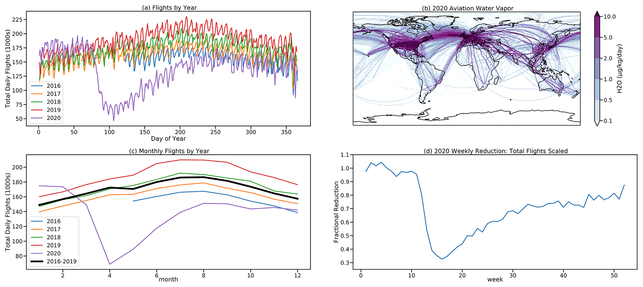
Figure 1(a) Daily total flights from 2016–2020. (b) Map of 2020 flight level water vapor emissions (micrograms per kilogram per day – µg kg−1 d−1). (c) Monthly average flights for each year and the 2016–2019 average (thick black line). (d) Scaled weekly estimate of the COVID-19-affected flight fraction for 2020.
This study will document the updated version of the contrail model that is publicly available as part of the Community Earth System Model, version 2.2, and its contrail effective radiative forcing (ERF) for a “normal” aviation in year 2020 with no pandemic reductions. We then use estimates of the changes in aviation emissions for the full year of 2020 to estimate changes in the contrail ERF due to the COVID-19 pandemic. ERF includes fast temperature adjustments due to changes in cloud formation and is the usual metric for understanding and assessing changes in the Earth's radiation budget.
Section 2 contains the methodology of the model and simulations, Sect. 3 contains results of the simulations, and conclusions are in Sect. 4.
2.1 Model
Simulations use the Community Earth System Model, version 2 (CESM2; Danabasoglu et al., 2020). The atmospheric model in CESM is the Community Atmosphere Model version 6.2 (CAM6; Gettelman et al., 2020). CAM6 uses a detailed two-moment cloud microphysics scheme (Gettelman and Morrison, 2015) coupled to an aerosol microphysics and chemistry model (Liu et al., 2016), as described by Gettelman et al. (2019).
To the standard version of CESM, we add the contrail parameterization of Chen et al. (2012) that was developed for CAM5. Since the ice cloud microphysics and aerosols are not substantially different between CAM5 and CAM6, the translation is straightforward. As described by Lee et al. (2021), we adjust the assumed emission ice particle diameter to 7.5 µm from the original parameterization (10 µm) to better align with the observations. The representation of contrails in CESM, described by Chen et al. (2012) and Chen and Gettelman (2013), adds aviation emissions of water vapor. A specified mass of water vapor is emitted based on a data set of total aircraft distance traveled, assuming a contrail diameter of 100 m over the grid box length and standard emission indices for commercial aircraft (see Chen et al., 2012 for details). If the temperature and humidity conditions indicate contrail formation (Appleman, 1953; Schumann, 1996), then the vapor is converted to ice crystals with a specified initial particle size of 7.5 µm (assuming small spherical ice crystals), yielding an ice number concentration increase. If conditions do not imply contrail formation, then water vapor is added. The vapor or ice is then is part of the fully conservative CESM hydrologic cycle with all microphysical processes active. When ice is formed, a 100 m wide cloud is added to the cloud fraction (for 100 km horizontal resolution, the cloud fraction added is thus 0.1 % per aircraft). The cloud then becomes part of the model hydrologic cycle and can persist and evolve or evaporate as subsequent time steps lasting from 30 min to many hours. The model can, thus, simulate linear contrails (representing a small cloud fraction in a model grid box), their evolution into contrail cirrus, and their effect on the background environment and existing clouds. For this study, we focus only on the impact of aviation water vapor emissions. Aviation aerosols may have substantial effects on subsequent cloud formation (Gettelman and Chen, 2013) but are highly uncertain (Lee et al., 2021), and we will focus solely on the effects of water vapor.
For CESM, we use the standard 32 levels (to 3 hPa) vertical and ∼ 1∘ horizontal resolution. Winds are nudged, as described by Gettelman et al. (2020) and Gettelman et al. (2021). The model time step is 1800 s. Winds and optional temperatures are relaxed to NASA Modern-Era Retrospective analysis for Research and Applications, version 2 (MERRA2; Molod et al., 2015), available every 3 h. The linear relaxation time is 24 h. CESM2 has a fully interactive land surface model (the Community Land Model, version 5; Danabasoglu et al., 2020). Sea surface temperatures (SSTs) are fixed to MERRA2 SST, and there is no interactive ocean.
These simulations permit temperature adjustment. Resulting radiative flux perturbations constitute an ERF. We also conduct sensitivity tests, as discussed below, where temperatures are nudged to MERRA2.
We have compared the results to previous contrail simulations with this model and others, as well as with observations. The pattern of the resulting contrail changes (illustrated below) to cloud fraction are very similar to the previous model documented in CAM5 (Chen and Gettelman, 2013, their Fig. 5), with peak effects in Northern Hemisphere mid-latitudes. The radiative forcing of the CAM6 simulations (discussed in detail below) is larger than in (Chen and Gettelman, 2013) due to the (a) smaller (100 vs. 300 m) initial contrail area and (b) smaller initial ice crystal sizes (7.5 vs. 10 µm diameter). The radiative forcing pattern and magnitude matches Bock and Burkhardt (2019, their Fig. 2a) qualitatively and quantitatively. This is consistent with the intercomparison between contrail simulation models that was recently conducted as part of the review by Lee et al. (2021). The CAM6 contrail model results also compare well to observations and simulations of contrails by Schumann et al. (2021a), who analyzed differences in clouds between 2020 and 2019. The CAM6 results have the same sign of cloud changes as observed and simulated in Schumann et al. (2021a). This yields further confidence in the CAM6 model estimates presented below.
2.2 Emissions data
To simulate aviation emissions for 2020 with and without COVID changes, we modify existing aviation inventories used with CESM. We take the Aviation Climate Change Research Initiative (ACCRI) 2006 inventory (Wilkerson et al., 2010) used with earlier versions of CESM (CAM5) (Chen et al., 2012; Gettelman and Chen, 2013). We focus only on water vapor emissions and contrails. We do not consider the effects of aviation aerosols in this study. The ACCRI 2006 inventory was developed based on detailed flight track data. The distribution of flight level water vapor emissions is shown in Fig. 1b. We make the assumption that air traffic has increased significantly since 2006, but that the flight locations and relative density have not changed drastically. In some rapidly developing regions of the planet, such as China, this assumption will result in some additional uncertainty.
To estimate the 2020 emissions, we estimate the growth in fuel use since 2006 as being equal to the growth in total aircraft distance traveled using data from Lee et al. (2021). Lee et al. (2021) report 54.7×10⁶ km of travel in 2018 and 33.2×10⁶ km in 2006. The scaling from 2006 to 2018 is then 1.58. We evaluate 2018–2020 increases in aviation emissions against aircraft movement data for total (commercial, private, and military) flights from Flightradar24 from 2016–2020 (available at https://www.flightradar24.com/data/statistics; last access: 15 January 2021; illustrated in Fig. 1). These data show growth over the last few years of 9 % per year. We, thus, use a 9 % per year increase over 2018–2020 (2 years) to generate a scaling from 2006 to 2020 of 1.88 (88 % increase from 2006) in a scenario without any COVID-19-induced reductions in aviation.
In order to determine the perturbation due to the COVID-19 lockdown, we use daily data for total flights for each day of 2020, provided by Flightradar24 and illustrated in Fig. 1a, and compare these data to a scaled-up average of previous years (2016–2019), which is 9 % above 2019 (Fig. 1c). We use weekly averages, since there is a strong weekly cycle in flights (Fig. 1a). Using daily averages would have required removing a weekly cycle to create scaling factors and then re-imposing it and assuming it was unchanged during the pandemic. The analysis yields a scaling value for every week of 2020 from our reference (scaled-up 2006 emissions), as illustrated in Fig. 1d. The first few weeks of 2020 were normal, then reductions started in February 2020, due to restrictions in China and Asia, and then in March (around week 12) as most nations introduced a lockdown period and most commercial flights were halted. Total aviation declined by two-thirds from what would have been expected. Recovery was rapid for about 10–15 weeks until the middle of 2020, and since then recovery has slowed, reaching approximately 75 %–80 % of the expected value by the end of 2020. Note that this value is total flights, including commercial (passenger and cargo), private, and military (with transponders) flights. The total load factor on passenger flights has decreased, so the total passenger miles flown is different to this. But it is total flights that are most relevant for water vapor emissions.
We then have a scaling factor for 2020 from 2006 (1.88) and weekly modifications to that factor for COVID-19-impacted emissions. These aviation water vapor emissions are used in our simulations to initiate contrails. All other emissions come from the Shared Socioeconomic Pathway (SSP) 245 emissions for 2019–2020 and are the same for all simulations.
2.3 Simulations
Full aviation simulations with 10 ensemble members are launched from 1 January 2019 to 31 December 2020 (2 years), with a small temperature perturbation (10−10 K). The initial perturbation results in a slightly different atmosphere evolution for each ensemble member. Nudging keeps the atmosphere in a similar “weather” state. The perturbation samples random fluctuations within that state. Critically, this enables estimates of the statistical significance of differences. We compared 10 and 20 ensemble members, and found that 10 members did not change the standard deviation or significance levels for full aviation emissions. We define the statistical significance for maps with the false discovery rate (FDR) method of Wilks (2006), which reduces patterned noise. We use the standard deviation across the ensembles to estimate uncertainty of and variability in global-averaged quantities. A similar methodology was used to examine non-aviation COVID-19-related aerosol emissions perturbations by Gettelman et al. (2021).
We run simulations with full aviation water vapor emissions (full air) and no aviation water vapor emissions (no air). We can analyze 2019 and 2020 effects with different meteorology in the 2-year simulations. As will be noted below, the land surface takes a few months to react to adjusted forcing (Fig. 2g), but the other variables adjust quickly (see Sect. 3.1). We also run an ensemble of 20 members, restarted on 1 January 2020, with COVID-19-reduced aviation water vapor emissions (COVID) for 2020. A total of 20 ensemble members are used due to the smaller perturbation. Finally, we also run a pair of 2020 ensembles with temperature nudging (full air T nudge; COVID T nudge) to explore how the evolution of temperature may affect the results.
First, we analyze global mean results by month in Sect. 3.1. We focus on the differences between ensembles with and without aviation or COVID-19-affected aviation for key climate parameters. Then we assess the spatial and seasonal distribution of these parameters (Sect. 3.2). This puts the overall global values into an important context for assessing contrail ERF and COVID-19 reductions in contrails. For clarity in dates, we will refer to the COVID-19-affected aviation simulations in the figures as “COVID”. Finally, we look in more detail at cloud changes and the effects of temperature nudging on the climate response to aviation contrails (Sect. 3.3).
3.1 Global mean results
Figure 2 illustrates monthly global mean quantities from the simulations. Shaded regions are 2 standard deviations (±2σ) across the ensemble. Global annual mean quantities are provided in Table 1. Figure 2 shows dates in 2020 but also illustrates the differences in the 2019 spin-up year (green solid lines; mapped to the 2020 annual cycle), which has the same aviation emissions but different meteorology. It is clear that the land surface temperature takes about 4 months to come to equilibrium with the forcing (Fig. 2h), but the other fields are all similar for all months.
Aviation contrails (full air − no air) cause increases in the negative SW cloud radiative effect (CRE), a net cooling (Fig. 2a), and a LW CRE warming (Fig. 2b; green, orange, and purple dashed lines). The opposite effects are seen when COVID-19 reductions (COVID − full Air) in contrails are assessed (blue and red dashed lines). There is an annual cycle in the SW CRE (Fig. 2a) with a peak cooling in the Northern Hemisphere (NH) summer, when maximum sunlight occurs in the regions of maximum emissions at NH mid-latitudes. The LW CRE (Fig. 2b) has virtually no annual cycle. The COVID-19 emissions changes should then be noted in the context of this annual cycle. The LW CRE changes due to COVID-19 reductions (Fig. 2b; blue solid and red dashed lines) clearly show differences that map directly to the temporal evolution of aviation reductions (Fig. 1d). The phase of the SW CRE (Fig. 2a) and LW CRE (Fig. 2b) for the COVID case do not exactly line up (peak SW in August; peak LW in April). This is because of the convolution between reductions (Fig. 1d), with the peak in the SW contrail effect (Fig. 2a).
The ice water path (IWP), due to full contrail effects (Fig. 2c), has a small annual cycle and is similar to LW CRE (Fig. 2b), which is sensitive to ice mass. The ratio of the LW CRE change to IWP change is similar for the 2020 full air (1.6), 2019 full air (1.6) and COVID (1.8) ensembles. There is little change relative to the variability in global average cloud top ice number (Fig. 2D), but this masks the regional variability which will be discussed below (Sect. 3.2). The average size of ice crystals decreases due to aviation contrails (Fig. 2e) and, correspondingly, increases when aviation contrails are reduced. This is expected as contrails add small (7.5 µm initial diameter) ice crystals into the model.
The changes in the high cloud (above 400 hPa) fraction are small (Fig. 2f). Few of the changes are significantly different from zero and mostly occur only in the summer period for full aviation emissions. There is a different annual cycle when temperature nudging is used (Fig. 2f; purple). These global changes mask the spatial and vertical structure in cloud field changes that we will analyze in Sect. 3.3.
The top of atmosphere (TOA) radiative flux (Fig. 2g) is a residual of positive LW CRE and negative SW CRE, with potential additional components due to possible effects of clouds on clear sky aerosols and surface temperature changes. In general, the LW CRE dominates; aviation contrails are a net warming effect over the annual cycle (Table 1), assessed at 33 or 90 mW m−2, depending on meteorology for 2020 and 2019 respectively. Combining the means and standard deviations yields an estimate of 62 ± 59 mW m−2 (±2σ range). This is very similar to the estimate from Lee et al. (2021) for 2018. Note that the COVID-19-reduced aviation emissions have offsetting LW and SW effects due to the timing of the aviation reductions such that the net global effect is actually positive but not distinguishable from zero (27 ± 58 mW m−2).
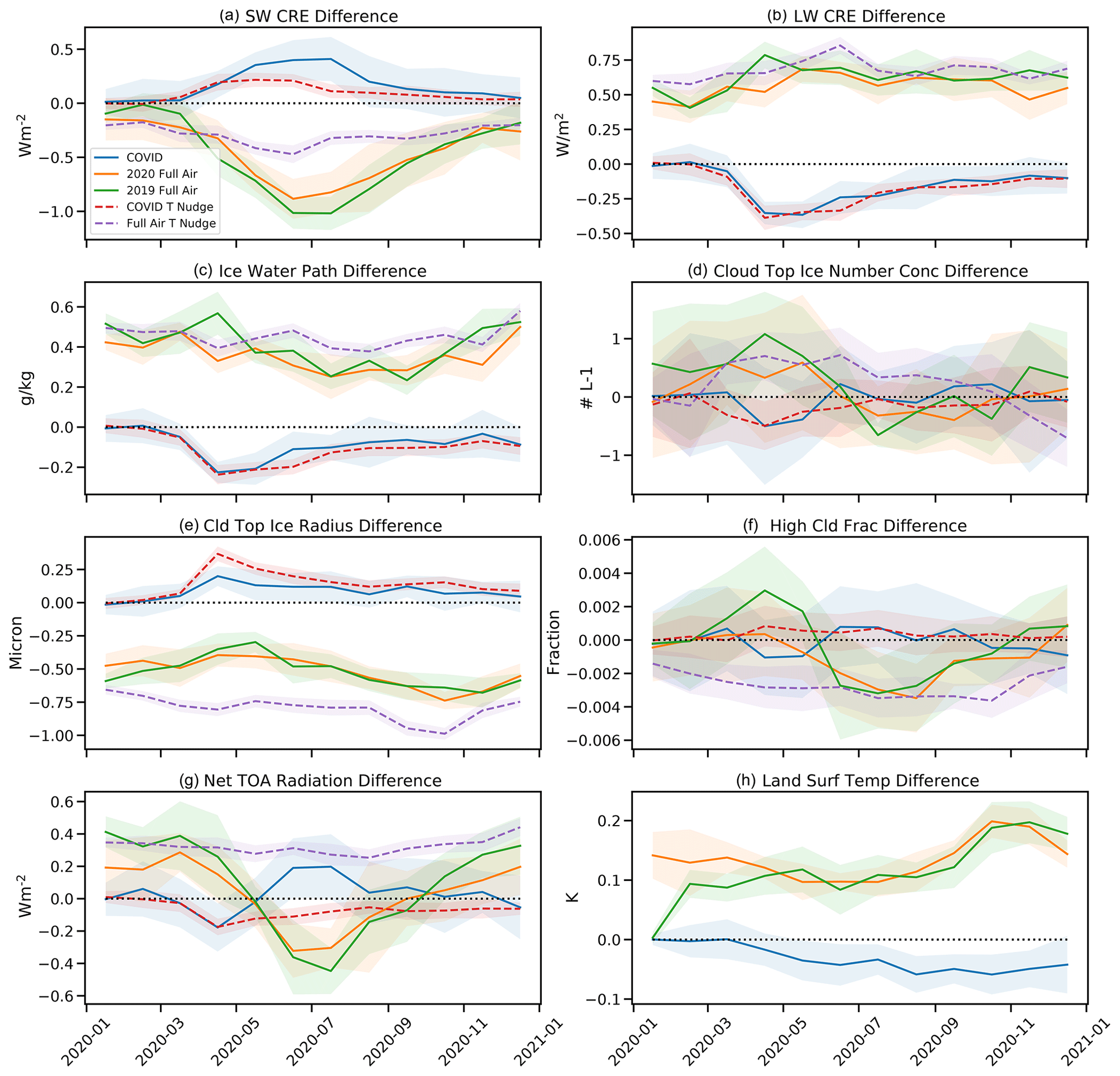
Figure 2Global monthly mean differences between sets of ensembles. Reductions due to COVID-19 aviation changes (COVID − full air; blue line), all aviation in 2020 (full air − no air; orange line), all aviation using 2019 meteorology (full air − no air; green line), COVID-19 changes with temperature nudging (COVID − full air; red dashed line), and full aviation with temperature nudging (full air − no air; purple dashed line). (a) Shortwave (SW) cloud radiative effect (CRE). (b) Longwave (LW) CRE. (c) Ice water path. (d) Cloud top ice number concentration (Cld top Ni). (e) Cloud top ice effective radius (Cld top Rei). (f) High cloud fraction (cld fract). (g) Net top of atmosphere (TOA) radiation difference. (h) Land surface temperature difference. Shading indicates 2 standard deviations of global means across the ensembles.
Table 1Global annual mean differences in the fields shown in Fig. 2. Uncertainties are 2 standard deviations across each ensemble.
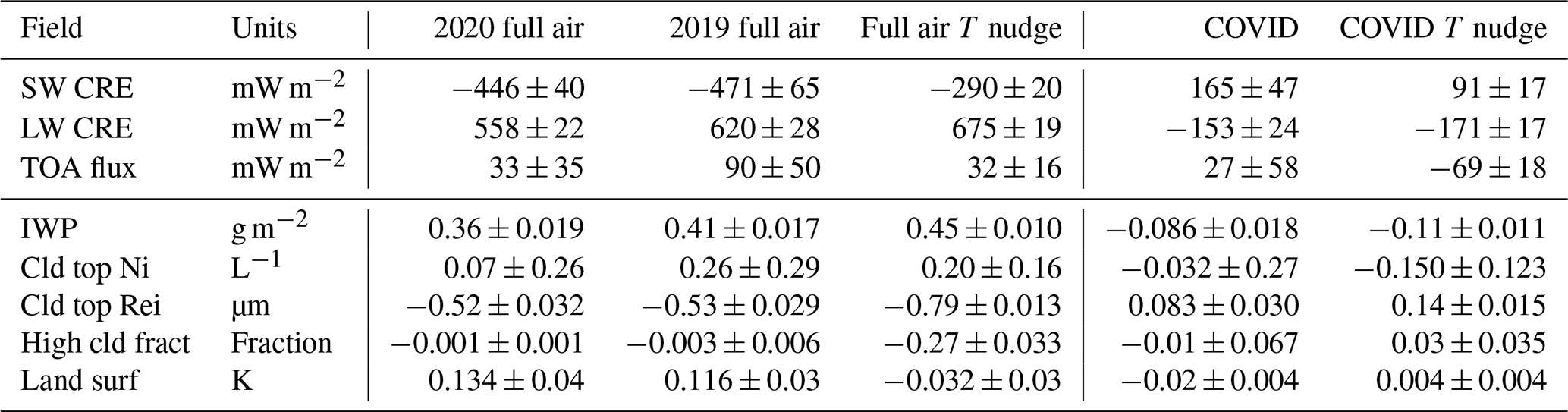
Even with these effects, there are very small but potentially significant changes in land surface temperature (Fig. 2h). Note that, because of limited land area and seasonal evolution, the land surface temperature changes may differ from net global TOA radiation changes. Note that these simulations assume zero temperature change over the ocean and, thus, do not include slow ocean feedbacks. However, the observed ocean temperatures are consistent (no additional forcing) with full aviation effects for 2019. Since the ocean adjustment time to any forcing is long, and the perturbations are much smaller than the variability in radiative forcing, any imbalance due to fixed ocean temperatures should be a small effect well within the uncertainty envelope of the ensemble. The 2019 simulations (Fig. 2h; green line) illustrate that the equilibration of the land surface takes 4 months or so. After 4 months, the 2020 and 2019 results are nearly identical for surface temperature. The atmospheric fields equilibrate much more rapidly, as seen in the similarity between the green (2019) and orange (2020) lines in Fig. 2a–g. The spatial structure will be assessed below. Thus, aviation contrails cause a significant land surface temperature warming averaged over the “normal” (no COVID-19 reductions) 2020 annual cycle of 0.13 ± 0.04 K. The COVID-19 reductions in aviation caused a cooling over land of −0.03 ± 0.03 K, even though there is no significant net TOA radiation difference (Fig. 2g and Table 1). This is understandable, based on the patterns of TOA flux, which are discussed below (Sect. 3.2).
3.2 Spatial patterns
Figure 3 illustrates the annual average spatial distribution of the climate quantities in Fig. 2 for the effect of full aviation contrails. Stippling indicates statistical significance at the 90 % level using the FDR methodology (Wilks, 2006). The expected pattern for many of the climate impacts matches the distribution of aircraft flight tracks (Fig. 1b), with peaks over eastern North America, Europe and Southeast and East Asia, as well as the North Atlantic and North Pacific oceans. A majority of the effects occur over the Northern Hemisphere. Contrails induce a cooling due to the SW CRE (Fig. 3a) and a co-incident warming due to LW CRE (Fig. 3b). This arises due to increases in the IWP (Fig. 3c). There are significant regional increases in ice number concentration (Fig. 3d), not evident in the global averages (Fig. 2d), which are concentrated where the IWP increases. The ice crystal size decreases (Fig. 3e) in a more diffuse but monotonic pattern, leading to a more consistent global decrease (Fig. 2e). A high cloud fraction has a more complex pattern of increases in the subtropics at flight altitudes, with decreases at higher latitudes over most of the Northern Hemisphere. This will be examined in more detail in Sect. 3.3 together with the vertical structure of cloud fraction and IWP changes.
The result of all of these changes is significant increases in TOA radiative flux (Fig. 3g) over parts of the Northern Hemisphere that are in or adjacent to flight lanes. Note that there are some significant remote decreases in TOA flux in regions with decreasing high clouds and negative LW and positive SW effects. So not only do LW and SW CRE effects of contrails cancel, but there are spatial regions of increasing and decreasing TOA flux. The resulting TOA fluxes over land lead to increases in land surface temperature nearly everywhere, peaking in the subtropical regions of Africa and Asia at 0.7 K. The pattern is not dependent on specific meteorology; similar patterns of warming are seen in western North America, subtropical Africa, the Middle East, and Asia with 2019 meteorology (not shown).

Figure 3Annual mean maps of differences in full air − no air for 2020. (a) Shortwave (SW) cloud radiative effect (CRE). (b) Longwave (LW) CRE. (c) Ice water path. (d) Cloud top ice number concentration. (e) Cloud top ice effective radius. (f) High cloud fraction. (g) Net top of atmosphere (TOA) radiation difference. (h) Land surface temperature difference. Stippled regions are significant differences using an FDR test at 90 % confidence.
The pattern of warming is due to the seasonal cycle, illustrated in Fig. 4. The lack of a significant annual mean warming signal over eastern North America and reduced signal over Europe is due to the seasonal cycle. There is warming in winter (December–February) over Europe and moderate warming over the USA, with cooling at higher latitudes. In summer (June–August), however, there is significant cooling over eastern North America and northern Europe. This arises from the seasonal cycle of TOA flux (Fig. 2g), which is negative in Northern Hemisphere summer due to strong SW CRE cooling from contrails (Fig. 2a), while the LW warming is more constant over the year (Fig. 2b). The TOA SW affects land temperatures directly in the absence of clouds, while the LW is filtered through the atmosphere; hence, the TOA net radiation affects the surface differently in different seasons.
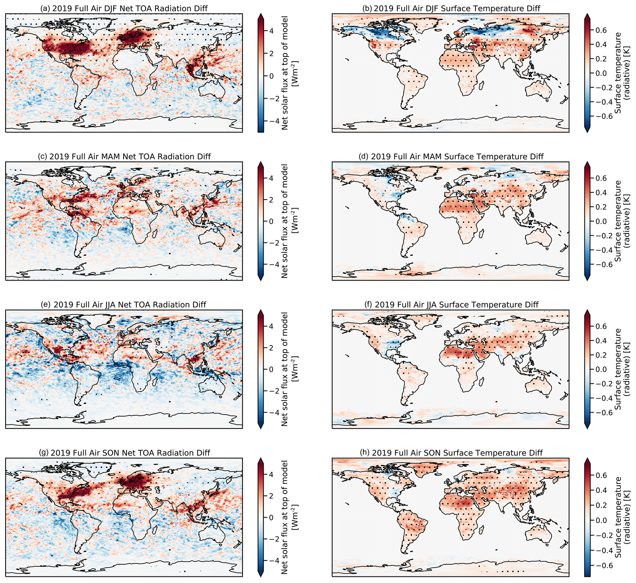
Figure 4Seasonal mean maps of differences in full air − no air for 2020. The left column (a, c, e, g) shows the TOA radiation, and the right column (b, d, f, h) shows the land surface temperature. (a, b) December–February (DJF), (c, d) March–May (MAM), (e, f) June–August (JJA), and (g, h) September–November (SON). Stippled regions are significant differences using an FDR test at 90 % confidence.
The changes due to COVID-19 reductions in contrails (Fig. 5) are as expected, i.e., they are smaller and of the opposite sign to the full contrail effect (Fig. 3) as contrails are reduced. The contour intervals in Fig. 5 are smaller than Fig. 3, so some of the ensemble variability (noise) appears, especially in the tropics (e.g., Fig. 5g). In general, similar patterns are seen in SW CRE (Fig. 5a), LW CRE (Fig. 5b), IWP (Fig. 5c), ice number (Fig. 5d), and ice effective radius (Fig. 5e). The high cloud differences are small (Fig. 5f) but also similar and opposite to full contrail effects. There is little significance to annual TOA radiation changes (Fig. 5g). Surface temperature over land cools as contrails are reduced (Fig. 5h). This has a similar and opposite pattern to the full contrail effects, including warming over the eastern USA and cooling over the western USA and in subtropical Africa and Asia, with the largest magnitude change −0.2 K. The cooling is due to compensating SW and LW effects that vary by season (Fig. 2).
In all these cases, the level of significance is small, indicating that the signal due to COVID-19-induced changes in contrails is smaller than variability in most regions. This makes comparisons to observations difficult. However, recent work (Quas et al., 2021) found that in the regions of highest air traffic density there was a 9 % decrease in expected cirrus cloud fraction in 2020. An analysis of MAM (March–May) for high cloud coverage (Fig. 5f) shows decreases in cirrus coverage up to 4 %–5 %, which is smaller than but consistent with observations.

Figure 5Annual mean maps of differences for COVID − full air for 2020. (a) Shortwave (SW) cloud radiative effect (CRE). (b) Longwave (LW) CRE. (c) Ice water path. (d) Cloud top ice number concentration. (e) Cloud top ice effective radius. (f) High cloud fraction. (g) Net top of atmosphere (TOA) radiation difference. (h) Land surface temperature difference. Stippled regions are significant differences using an FDR test at 90 % confidence.
3.3 Cloud changes and effects of temperature nudging
The spatial (Fig. 3f) and temporal (Fig. 2f) pattern of high cloud changes due to contrails shows significant effects away from flight routes. The vertical structure of the cloud changes, along with temperature and ice water path, are shown in Fig. 6. Aviation water vapor causes increases in cloud ice mass concentrations (Fig. 6c). This can increase or decrease the cloudiness (Fig. 6a) depending on the temperature (and humidity) response. Without temperature nudging, there is local warming due to LW absorption by cloud ice (Fig. 6b). The increase in temperature and cloud ice (Fig. 6c), some of which comes from forming contrails in supersaturated air and the subsequent uptake of environmental water, results in decreasing relative humidity (not shown) and, hence, decreases cloud fraction (Fig. 6a).
Nudging temperature alters the cloud response (Fig. 6d), with a larger decrease in clouds at mid-latitudes and reduced increases in cloudiness in the subtropics. The cloud ice mass response is similar with (Fig. 6c) or without (Fig. 6f) temperature nudging. The high cloud increases near the Equator are in the subtropics and mostly zonal (Fig. 3f) and may be associated with temperature increases allowing more water vapor and then cloud ice to be present. This highlights the subtle challenges of describing a radiative forcing, and why we use ERF that includes these local temperature responses. COVID-19 changes in clouds and ice without (Fig. 6g, h, j) and with (Fig. 6k, l, m) temperature nudging are similar to full aviation effects but are smaller and of the opposite sign.
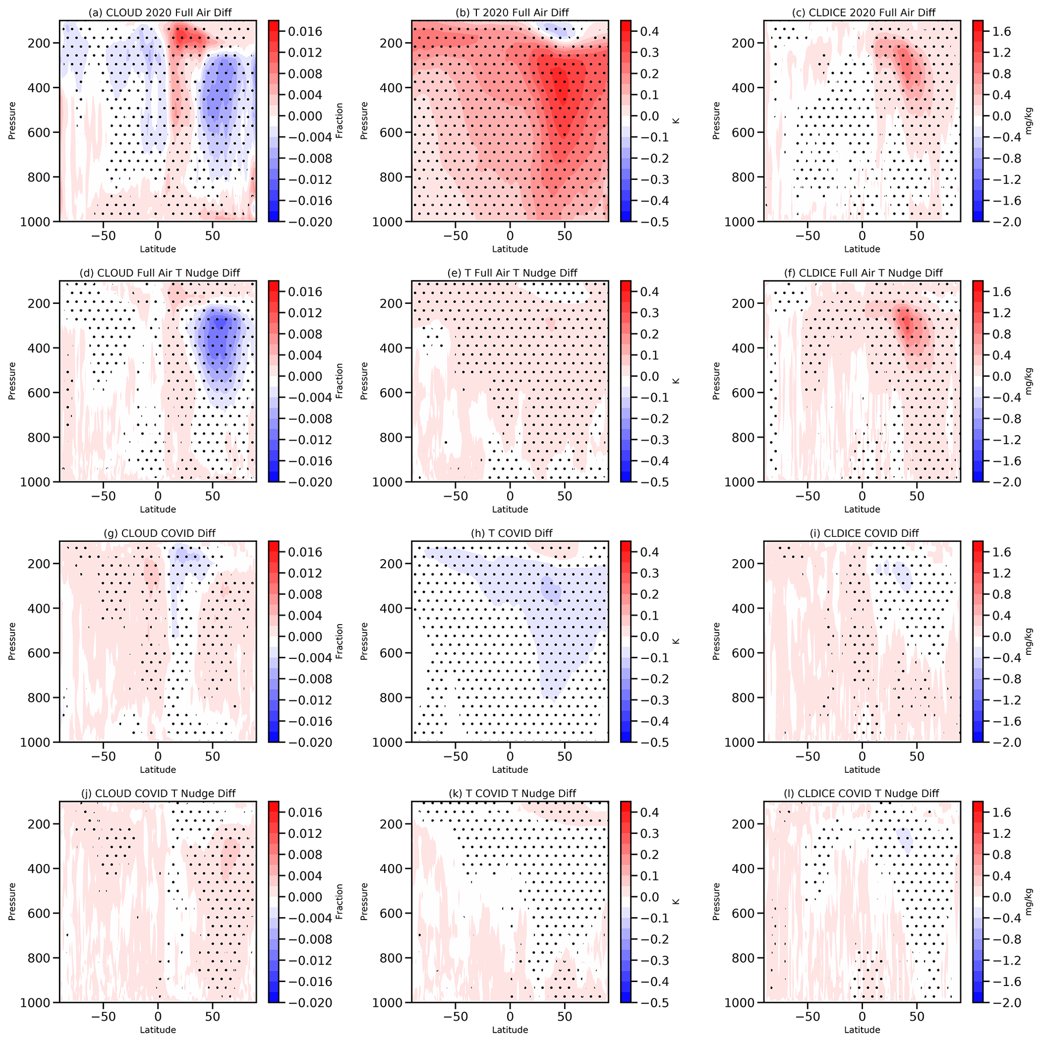
Figure 6Annual zonal mean latitude height plots differences in cloud fraction (a, d, g, k), temperature, T (b, e, h, l), and cloud ice mixing ratio (c, f, j, m). The panels show COVID − full air (a, b, c), no aviation − full air (d, e, f), no aviation − full aviation T nudged (g, h, i), and COVID − full aviation with T nudging (k, l, m). Stippled regions are significant differences using an FDR test at 90 % confidence.
These simulations of aviation contrails and the effect of COVID-19-induced reductions provide some interesting new perspectives on the effect of contrails on climate. Contrail effective radiative forcing (ERF) is estimated at 62 ± 59 mW m−2 (2σ) for current (2020) aviation in the absence of any COVID-19-pandemic-caused reductions. The variability range is due to the ensemble spread and differences in year-to-year meteorology, indicating that the value may vary from year to year. A more complete analysis of interannual variability should be conducted but is beyond the scope of this study. This range is well in line with recent assessments of contrail ERF (Lee et al., 2021). The specific differences between 2020 and 2019 compare well to observations and contrail simulations of Schumann et al. (2021a).
The net contrail ERF has complex spatial and seasonal patterns and is a residual of SW cooling and LW heating components nearly 10 times the net effect. The patterns are important to understand and demonstrate a significant complexity in the assessment of aviation contrail impacts. This arises because of the seasonality of SW radiation (Fig. 2a) mapped onto the seasonality of flights (Fig. 1), which results in net contrail cooling from June to September (Fig. 2g and Fig. 4e) but strong global (Fig. 2g) and regional (Fig. 4a) heating effects in December–February. This is an underappreciated part of the contrail ERF and may have implications for mitigation strategies.
The spatial and seasonal forcing variations also map onto land surface temperature variations, resulting in smaller annual temperature changes than might be expected. In western Europe, for example, peak net radiation differences occur in fall and winter when radiation is a smaller part of the surface energy budget, so little temperature change results. In eastern North America, the SW cooling effects of contrails dominate in spring and summer, while LW effects occur more strongly in fall and winter, such that there is little annual temperature change. The largest temperature changes are found over subtropical Africa, away from flight routes, but these regions are perhaps affected by high cloud increase due to the remote effects of aviation.
The temperature changes resulting from these small ERFs are much smaller than climate variability in a fully coupled system. For this study, ocean temperatures are fixed, which is fine in the short term and for small ERF estimates. With this caveat, there are significant increases in temperature over most land regions due to contrails, with an annual average over land of 0.13 ± 0.04 K. The peak annual temperature change is 0.7 K in the Northern Hemisphere subtropics.
The effect of COVID-19 reductions in flight traffic (Fig. 1d) decreased contrails. The unique timing of such reductions, which were maximum in Northern Hemisphere summer, when the largest contrail cooling occurs, means that warming reductions due to fewer contrails in the spring and fall were offset by cooling reductions due to fewer contrails in summer, giving no significant annual averaged ERF from contrail changes in 2020. Despite no net significant global ERF, there are some land regions that cooled significantly and up to −0.2 K from what would have been expected with baseline aviation contrails. These reductions occurred in the same regions as large contrail temperature changes in the subtropical Northern Hemisphere.
The patterns of surface warming and cooling are not exactly coincident with contrail ERF, indicating distributed effects through the climate system. These effects should be further tested and not just with a coupled land surface (as has been done here) but with a coupled ocean. However, this will introduce additional climate noise as well, so is a subject for future work.
This study has not considered any impacts of changes to aviation aerosol emissions, largely sulfate (SO4) and black carbon (BC). Aviation aerosols are highly uncertain, which is why we chose to focus on aviation water vapor. Note that aviation aerosols affect only subsequent cloud formation and not initial contrails and contrail cirrus. In CESM, aviation aerosols, especially SO4, tend to mix downward to affect liquid clouds below (Gettelman and Chen, 2013). The net effect of the aviation aerosols is cooling, so COVID-19 reductions would likely cause a net warming. The seasonality is similar to the SW effects here. But these effects have not been included because there is a wide divergence in the outcomes, depending on the model and the background state of cirrus cloud microphysics. These aerosol mechanisms have yet to be confirmed and are not yet quantified – even in recent assessments (Lee et al., 2021).
This study provides estimates based on unique and detailed modeling frameworks to elucidate small changes in the climate system with ensembles of constrained simulations. One important question is whether any of these simulated changes due to COVID-19 aviation reductions can be seen in observations. The pattern and timing of radiation and warming changes might yield sufficient fingerprints in instrumental records of anomalies during 2020 to be able to tease out these effects, and this an interesting avenue for future research. Preliminary work (Quas et al., 2021) indicates observed decreases in cloud fraction in 2020 in high traffic regions consistent with these simulations. This is one avenue for a comparison of these simulations to the observations. Other analyses are possible, and simulation results are available to the community for further analysis.
What does this analysis mean for the future climate impact of contrails? The cancellation between LW and SW indicates that the spatial and seasonal distribution of flights may change the contrail ERF. Local effects in space and time may not be the same as global impacts due to the timing of contrails and solar insolation. If flights increase in tropical regions where there is more SW radiation throughout the year, this might decrease the ERF of contrails (more cooling). But it also may mean more flights in regions susceptible to contrails, such as the upper troposphere (through regions of ice supersaturation). An updated aviation emissions database (more recent than the scaled 2006 ACCRI inventory used here) and projections would be useful to begin these assessments. The results here also indicate that the seasonal cycle could be used as a contrail mitigation strategy, whereby one would not want to alter or reduce contrails in regions and during certain times of the year with larger SW cooling.
Simulation output and modified code used in this analysis are available at https://doi.org/10.5281/zenodo.4584078 (Gettelman, 2021). Simulations are based on CAM6.2, which is available from https://github.com/ESCOMP/CAM/tree/cam6_2_022 (ESCOMP, 2021).
AG designed the study, did the main simulations and analysis, and wrote the paper. CCC modified the code, did the preliminary simulations and analysis, and helped edit the paper. CGB assisted with the data sets and editing of the paper.
The authors declare that they have no conflict of interest.
The National Center for Atmospheric Research is funded by the U.S. National Science Foundation. Thanks to Flightradar24 for access to the total flight data. Thanks to David S. Lee, for the discussion and analysis of aviation emissions growth. Thanks also to Ulrich Schumann, for the detailed discussions of the recent work on observing cloud changes during 2020.
This paper was edited by Pedro Jimenez-Guerrero and reviewed by Donald Wuebbles and one anonymous referee.
Appleman, H. S.: The Formation of Exhaust Condensation Trails by Jet Aircraft, B. Am. Meteorol. Soc., 34, 14–20, 1953. a
Bock, L. and Burkhardt, U.: Contrail cirrus radiative forcing for future air traffic, Atmos. Chem. Phys., 19, 8163–8174, https://doi.org/10.5194/acp-19-8163-2019, 2019. a
Chen, C.-C. and Gettelman, A.: Simulated radiative forcing from contrails and contrail cirrus, Atmos. Chem. Phys., 13, 12525–12536, https://doi.org/10.5194/acp-13-12525-2013, 2013. a, b, c
Chen, C. C., Gettelman, A., Craig, C., Minnis, P., and Duda, D. P.: Global Contrail Coverage Simulated by CAM5 with the Inventory of 2006 Global Aircraft Emissions, J. Adv. Model. Earth Sy., 4, M04003, https://doi.org/10.1029/2011MS000105, 2012. a, b, c, d
Danabasoglu, G., Lamarque, J.-F., Bacmeister, J., Bailey, D. A., DuVivier, A. K., Edwards, J., Emmons, L. K., Fasullo, J., Garcia, R., Gettelman, A., Hannay, C., Holland, M. M., Large, W. G., Lauritzen, P. H., Lawrence, D. M., Lenaerts, J. T. M., Lindsay, K., Lipscomb, W. H., Mills, M. J., Neale, R., Oleson, K. W., Otto-Bliesner, B., Phillips, A. S., Sacks, W., Tilmes, S., van Kampenhout, L., Vertenstein, M., Bertini, A., Dennis, J., Deser, C., Fischer, C., Fox-Kemper, B., Kay, J. E., Kinnison, D., Kushner, P. J., Larson, V. E., Long, M. C., Mickelson, S., Moore, J. K., Nienhouse, E., Polvani, L., Rasch, P. J., and Strand, W. G.: The Community Earth System Model Version 2 (CESM2), J. Adv. Model. Earth Sy., 12, e2019MS001916, https://doi.org/10.1029/2019MS001916, 2020. a, b
ESCOMP: CAM: The Community Atmosphere Model, GitHub, available at: https://github.com/ESCOMP/CAM/tree/cam6_2_022, last access: 11 June 2021. a
Forster, P. M., Forster, H. I., Evans, M. J., Gidden, M. J., Jones, C. D., Keller, C. A., Lamboll, R. D., Quéré, C. L., Rogelj, J., Rosen, D., Schleussner, C.-F., Richardson, T. B., Smith, C. J., and Turnock, S. T.: Current and Future Global Climate Impacts Resulting from COVID-19, Nat. Clim. Change, 10, 913–919, https://doi.org/10.1038/s41558-020-0883-0, 2020. a
Gettelman, A.: Simulations of Contrails Under COVID-19 Effects, Zenodo [data set and code], Zenodo, https://doi.org/10.5281/zenodo.4584078, 2021. a
Gettelman, A. and Chen, C.: The Climate Impact of Aviation Aerosols, Geophys. Res. Lett., 40, 2785–2789, https://doi.org/10.1002/grl.50520, 2013. a, b, c
Gettelman, A. and Morrison, H.: Advanced Two-Moment Bulk Microphysics for Global Models. Part I: Off-Line Tests and Comparison with Other Schemes, J. Climate, 28, 1268–1287, https://doi.org/10.1175/JCLI-D-14-00102.1, 2015. a
Gettelman, A., Hannay, C., Bacmeister, J. T., Neale, R. B., Pendergrass, A. G., Danabasoglu, G., Lamarque, J.-F., Fasullo, J. T., Bailey, D. A., Lawrence, D. M., and Mills, M. J.: High Climate Sensitivity in the Community Earth System Model Version 2 (CESM2), Geophys. Res. Lett., 46, 8329–8337, https://doi.org/10.1029/2019GL083978, 2019. a
Gettelman, A., Bardeen, C. G., McCluskey, C. S., Järvinen, E., Stith, J., Bretherton, C., McFarquhar, G., Twohy, C., D'Alessandro, J., and Wu, W.: Simulating Observations of Southern Ocean Clouds and Implications for Climate, J. Geophys. Res.-Atmos., 125, e2020JD032619, https://doi.org/10.1029/2020JD032619, 2020. a, b
Gettelman, A., Gagne, D. J., Chen, C.-C., Christensen, M. W., Lebo, Z. J., Morrison, H., and Gantos, G.: Machine Learning the Warm Rain Process, J. Adv. Model. Earth Sy., 13, e2020MS002268, https://doi.org/10.1029/2020MS002268, 2021. a, b, c
Le Quéré, C., Jackson, R. B., Jones, M. W., Smith, A. J. P., Abernethy, S., Andrew, R. M., De-Gol, A. J., Willis, D. R., Shan, Y., Canadell, J. G., Friedlingstein, P., Creutzig, F., and Peters, G. P.: Temporary Reduction in Daily Global CO2 Emissions during the COVID-19 Forced Confinement, Nat. Clim. Change, 10, 647–653, https://doi.org/10.1038/s41558-020-0797-x, 2020. a
Lee, D. S., Fahey, D. W., Skowron, A., Allen, M. R., Burkhardt, U., Chen, Q., Doherty, S. J., Freeman, S., Forster, P. M., Fuglestvedt, J., Gettelman, A., De León, R. R., Lim, L. L., Lund, M. T., Millar, R. J., Owen, B., Penner, J. E., Pitari, G., Prather, M. J., Sausen, R., and Wilcox, L. J.: The Contribution of Global Aviation to Anthropogenic Climate Forcing for 2000 to 2018, Atmos. Environ., 244, 117834, https://doi.org/10.1016/j.atmosenv.2020.117834, 2021. a, b, c, d, e, f, g, h, i, j
Liu, X., Ma, P.-L., Wang, H., Tilmes, S., Singh, B., Easter, R. C., Ghan, S. J., and Rasch, P. J.: Description and evaluation of a new four-mode version of the Modal Aerosol Module (MAM4) within version 5.3 of the Community Atmosphere Model, Geosci. Model Dev., 9, 505–522, https://doi.org/10.5194/gmd-9-505-2016, 2016. a
Molod, A., Takacs, L., Suarez, M., and Bacmeister, J.: Development of the GEOS-5 atmospheric general circulation model: evolution from MERRA to MERRA2, Geosci. Model Dev., 8, 1339–1356, https://doi.org/10.5194/gmd-8-1339-2015, 2015. a
Quaas, J., Gryspeerdt, E., Vautard, R., and Boucher, O.: Climate Impact of Aircraft-Induced Cirrus Assessed from Satellite Observations before and during COVID-19, Environ. Res. Lett., 16, 064051, https://doi.org/10.1088/1748-9326/abf686, 2021. a, b
Schumann, U.: On Conditions for Contrail Formation from Aircraft Exhausts (Review Article), Meteorol. Z., 5, 4–23, 1996. a
Schumann, U., Bugliaro, L., Dörnbrack, A., Baumann, R., and Voigt, C.: Aviation Contrail Cirrus and Radiative Forcing Over Europe During 6 Months of COVID-19, Geophys. Res. Lett., 48, e2021GL092771, https://doi.org/10.1029/2021GL092771, 2021a. a, b, c
Schumann, U., Poll, I., Teoh, R., Koelle, R., Spinielli, E., Molloy, J., Koudis, G. S., Baumann, R., Bugliaro, L., Stettler, M., and Voigt, C.: Air traffic and contrail changes over Europe during COVID-19: a model study, Atmos. Chem. Phys., 21, 7429–7450, https://doi.org/10.5194/acp-21-7429-2021, 2021b. a
Wilkerson, J. T., Jacobson, M. Z., Malwitz, A., Balasubramanian, S., Wayson, R., Fleming, G., Naiman, A. D., and Lele, S. K.: Analysis of emission data from global commercial aviation: 2004 and 2006, Atmos. Chem. Phys., 10, 6391–6408, https://doi.org/10.5194/acp-10-6391-2010, 2010. a
Wilks, D. S.: On “Field Significance” and the False Discovery Rate, J. Appl. Meteor. Climatol., 45, 1181–1189, https://doi.org/10.1175/JAM2404.1, 2006. a, b