Event Forecasting for Thailand’s Car Sales during the COVID-19 Pandemic

Abstract

The COVID-19 pandemic that started in 2020 has affected Thailand’s automotive industry, among many others. During the several stages of the pandemic period, car sales figures fluctuate, and hence are difficult to fit and forecast. Due to the trend present in the sales data, the Holt’s forecasting method appears a reasonable choice. However, the pandemic, or in a more general term, the “event”, requires a subtle method to handle this extra event component. This research proposes a forecasting method based on Holt’s method to better suit the time-series data affected by large-scale events. In addition, when combined with seasonality adjustment, three modified Holt’s-based methods are proposed and implemented on Thailand’s monthly car sales covering the pandemic period. Different flags are carefully assigned to each of the sales data to represent different stages of the pandemic. The results show that Holt’s method with seasonality and events yields the lowest MAPE of 8.64%, followed by 9.47% of Holt’s method with events. Compared to the typical Holt’s MAPE of 16.27%, the proposed methods are proved strongly effective for time-series data containing the event component.

1. Introduction

The automotive industry has been one of the most blossoming industries in Thailand for decades in both production and sales dimensions, owing to several factors. For the production dimension, Thailand is a crucial automobile part manufacturer and at the same time, an assembly hub for the Southeast Asia region [1], even though Thailand does not own any internationally renowned car brands.

Regarding the sales dimension, Bangkok, the capital city, is always among the top worst traffic cities in the world [2,3]. The majority of middle-class Thai citizens are in need of vehicles to commute between home in the suburban areas and workplace in the city on account of insufficient and inconvenient public transportation systems. Besides pick-up trucks widely used for commercials, the best-selling vehicle types for ordinary Thai citizens are compact and subcompact sedans, with engines up to 1800 c.c. [4].

Beginning in early 2020, Thailand was among the first countries attacked by the coronavirus disease or COVID-19 [5]. As was the case for every other place in the world, Thailand’s economy rapidly decreased as the virus developed into a global pandemic. Millions of people were at risk of losing their jobs, earning less salaries, and gaining reduced or no bonuses [6,7]. Consequently, every household tried to save their incomes to make ends meet, especially for the rainy days, and thus decreased the unnecessary consumption. A new car purchase was obviously on the unnecessary buying list, attributable to a certain characteristic of the cars being depreciated assets. To make the matter even worse, all the businesses, automotives included, were heavily affected by the nationwide lockdowns initiated by the government to prevent the disease spreading.

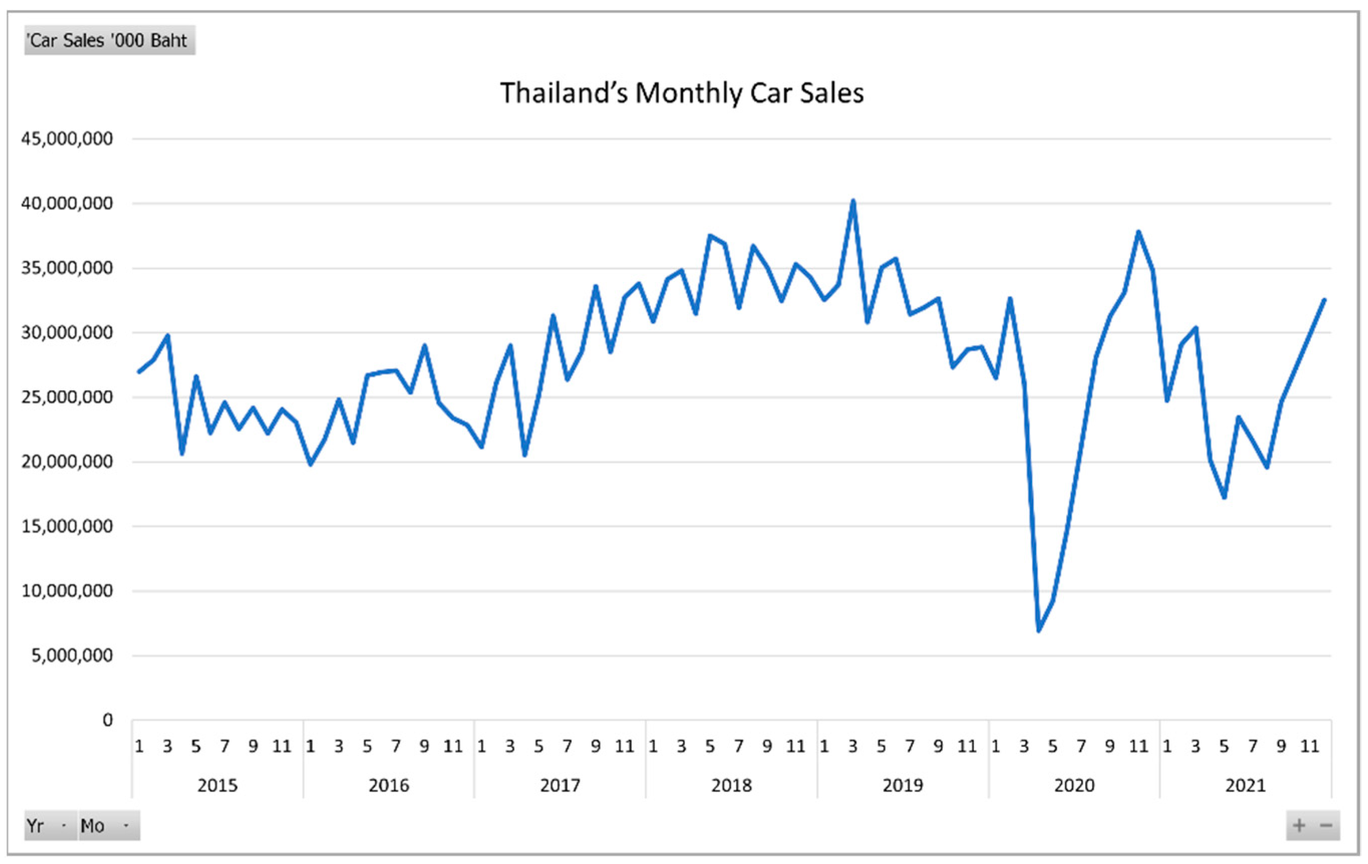
In Figure 1, Thailand’s monthly car sales from January 2015 to December 2021 are depicted. During the first COVID-19 superspreading wave across the nation, approximately for the first to the mid-third quarters of 2020, the sales curve declined drastically, especially from March to April, before gradually entering a relief period. However, the nation and the entire world had not experienced the end of the pandemic yet. Superspreading waves 2 and 3 struck in the following months, making car sales unsteady all over again. From an optimistic point of view, as the new car sales figures continue to progress into 2022, the situation will eventually return to normal in the near future.

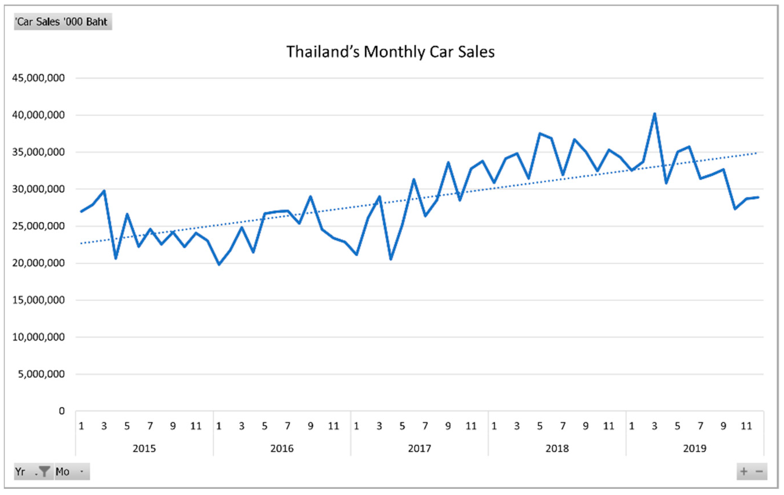
In Figure 2, the monthly car sales data are trimmed to show only from the normal period, in other words, no COVID-19 pandemic effects, i.e., from January 2015 to December 2019. Evidently, the added trendline exhibits an upward trend, in which the time-series Holt’s or double exponential smoothing method are, thus, appropriate methods to start with [8]. However, the full car sales data in Figure 1 are severely disturbed by the pandemic. Consequently, the typical Holt’s method may not perform as well as intended. Thus, in this research, modifications of the Holt’s method are proposed to incorporate the effects of the pandemic, or the more general term, “the event component”.

Furthermore, to gain even higher accuracy forecasts, the seasonal component in the car sales data is also integrated into the proposed modifications. In total, the typical Holt’s method, along with the three modified methods, namely, Holt’s method with seasonality, Holt’s method with events, and Holt’s method with seasonality and events, will be used for Thailand’s monthly car sales from January 2015 to December 2021. Then, their accuracies, using the mean absolute percentage error (MAPE) and the symmetric mean absolute percentage error (SMAPE), will be computed and compared.

2. Literature Review

Previous work regarding forecasting methods and the event component is surveyed and presented as follows.

Wirotcheewan et al. [9] found a suitable forecasting model for the advanced demand of the automotive wheels, parts, and accessories (WPA), and used a linear programming (LP) model to calculate the optimal quantity for export so as to gain from the maximum profit. The WPA demands for export from Thailand are collected from the top five highest-demand countries, i.e., Japan, China, South Korea, Germany, and Indonesia from 1997 to 2008. Time series forecasting models used in the study are naïve, moving average, single exponential smoothing, and exponential smoothing with trend or Holt’s method and artificial neural networks (ANNs). The forecasting accuracy measurement is MAPE. The results show that the ANNs model outperforms the other models for Japan, Germany, and Indonesia, while exponential smoothing with trend is best suited for China. Nonetheless, all five models produce MAPEs greater than 50% for South Korea. After that, the forecasted results are used in finding the optimal quantities for export to those five countries using LP models.

Rattanametawee et al. [10] study the effects of special events on regression for subcompact car sales in Thailand. The monthly input data are collected from January 2005 to September 2015, summing to 129 data. The two special events considered are the 2011 Thailand flood and the government’s tax-incentive first-car buyer program in 2011–2012. For the methodology, they use three different multiple linear regressions, specifically, the regular regression, regression containing seasonality, and the proposed regression containing seasonality and special events. The results show that the last regression outperforms the other two models and achieves the highest adjusted coefficient of determination or R-square and also the highest accuracy in terms of MAPE.

Booranawong and Booranawong [11] use double exponential smoothing (DES) or Holt’s methods, multiplicative Holt–Winters (MHW) and additive Holt–Winters (AHW) with optimal initial values and smoothing constants to forecast lime, Thai chili and lemongrass prices in Thailand from October 2016 to December 2016. This research collects the input price data at the Simummuang market from January 2011 to September 2016. The accuracy measure for comparisons is MAPE. The results show that DES attains the smallest MAPEs for forecasting Thai chili and lemongrass prices, while MHW and AHW generate smaller MAPEs than that of DES for forecasting lime prices possessing the seasonal component.

Muchayan [12] uses two different double exponential smoothing methods, namely, Brown’s and Holt’s, to predict the net asset value (NAV) price movements of the Cipta Ovo Equitas mutual fund from the Ciptadana Asset Management, PT in Indonesia. The NAV price data are collected over the period January 2019 to January 2020. The measurement of effectiveness is MAPE. The results show that Holt’s method yields a smaller MAPE than Brown’s method.

Sharif and Hasan [13] develop a stock indicator that helps buyers predict the next day’s share value by applying the Holt’s method. The stock closing prices of different companies are gathered from the Dhaka Stock Exchange (DSE) in 2016. This study finds that the Holt’s method is appropriate for short-term prediction. In addition, this study shows that different smoothing constants have an impact on the prediction values and the proper values of smoothing constants for this dataset are α = 0.5 and β = 0.1.

Suppalakpanya et al. [14] study several exponential smoothing methods for forecasting crude palm oil productions in Thailand from January 2018 to March 2018. The monthly crude palm oil productions data are collected from the database of the Department of Internal Trade, Ministry of Commerce, Thailand. This research compares five different forecasting methods for various ranges of the input data. The first three methods are double exponential smoothing (DES), the multiplicative Holts–Winters (MHW), and the additive Holt–Winters (AHW) methods. Additionally, their proposed modified methods are the improved additive Holts–Winters (IAHW) and the extended additive Holts–Winters (EAHW) methods. For the input ranges, they implement all the five methods on four different ranges, i.e., 3-year data (2015–2017), 6-year data (2012–2017), 9-year data (2009–2017), and 12-year data (2006–2017). The accuracy measurement is MAPE. The results show that the AHW and EAHW methods yield the two lowest MAPEs of 6.94 and 7.05, respectively, when the 12-year data are applied.

Rattanametawee and Leenawong [15] propose a new time-series decomposition to incorporate the effects of special events that impact the dataset. They use a case study of subcompact monthly car sales data in Thailand from 2011 to 2018. This dataset has the conventional trend, seasonal, and cyclical components. The special events investigated in the study are the tax-incentive program for first car buyers having a positive impact on the data, and the national big flood having, in contrast, a negative impact. MAPE is used as an accuracy measure of the proposed forecasting method, resulting in a relatively low value at 8.17%.

With regard to the organization of this paper, in the next section, the typical Holt’s method along with the modified methods are explained in detail and their formulas are shown explicitly, including the accuracy measurement. In Section 4, the experimental results and their discussion are provided. Then, in the final Section 5, this research is concluded.

3. Materials and Methods

In this section, all forecasting methods are explicitly described to be implemented on Thailand’s monthly car sales data from January 2015 to December 2021. The data are collected from the Office of Industrial Economics, Ministry of Industry, Thailand [16]. Note that all the experiments are conducted on Microsoft Excel 365.

3.1. The Typical Holt’s Method

First of all, common notations to be used in this typical Holt’s method and its subsequent modified methods are defined as follows.

A_t represents the actual data for period t,

α represents the smoothing constant for the level estimate; 0 ≤ α ≤ 1,

and β represents the smoothing constant for the trend estimate; 0 ≤ β ≤ 1.

The typical Holt’s forecasting method can be executed by the following three steps [17].

• Step 1: Computing the Level Estimate.

L_t = αA_t + (1 − α) (L_t−1 + T_t−1)

(1)

where L_t refers to the level estimate for period t, T_t refers to the trend estimate for period t, and the initial value for L_t is L₂ = A₂, and for T_t is T₂ = A₂ − A₁.

• Step 2: Computing the Trend Estimate.

T_t = β (L_t − L_t−1) + (1 − β) T_t−1

(2)

• Step 3: Computing the Holt’s Estimate.

H_t+m = L_t + mT_t

(3)

where H_t+m refers to Holt’s forecasted value for period t + m, and m refers to the future period mth; m ≥ 1.

In the next section, the forecasting steps of the Holt’s method with seasonality will be described.

3.2. The Holt’s Method with Seasonality

The forecasting steps of the typical Holt’s method are modified to take into consideration the seasonality in the data. Some steps are changed and two additional steps are inserted to account for the seasonal component and it, thus, comes to a total of five steps. Note that certain notations used in some steps of the typical Holt’s method are slightly altered to reflect the seasonality in the data as well. In conclusion, the Holt’s method with seasonality can be executed by the following five main steps.

• Step 1 (Additional): Dealing with Seasonality.

In this new step, for the original data with a seasonal component, it is advised that the seasonal component is first removed or de-seasonalized before performing Holt’s method. Then, after obtaining the forecasted values from Holt’s method, these Holt’s forecasts must be incorporated back or re-seasonalized in the very last stop to reach the final forecasts. In doing so, seasonal indices are required and they are determined by the following sub-steps, 1.1–1.5. In the last sub-step 1.6, the seasonal indices are used to remove the seasonal component from the original data.

• Step 1.1: Finding the Moving Averages (MAs).

A_y,m represents the actual data of year y, month m, where y = 1, 2, …, 7 refer to the years 2015, 2012, …, 2021 and m = 1, 2, …, 12 refer to the months January, February, …, and December, respectively, and ${\overline{\mathrm{A}}}_{\mathrm{y},\mathrm{m}}$ represents the moving average of year y, month m, when the number of periods to average is 12.

Therefore, the values start at ${\overline{\mathrm{A}}}_{1,6}$ up until ${\overline{\mathrm{A}}}_{7,6}$. More explicitly [18],

$$\begin{gathered} {\overline{\mathrm{A}}}_{1,6}=\left({\mathrm{A}}_{1,1}+{\mathrm{A}}_{1,2}+\dots +{\mathrm{A}}_{1,12}\right)/12, \\ {\overline{\mathrm{A}}}_{1,7}=\left({\mathrm{A}}_{1,2}+{\mathrm{A}}_{1,3}+\dots +{\mathrm{A}}_{1,12}+{\mathrm{A}}_{2,1}\right)/12, \\ {\overline{\mathrm{A}}}_{1,8}=\left({\mathrm{A}}_{1,3}+{\mathrm{A}}_{1,4}+\dots +{\mathrm{A}}_{1,12}+{\mathrm{A}}_{2,1}+{\mathrm{A}}_{2,2}\right)/12, \\ ⋮ \\ {\overline{\mathrm{A}}}_{7,6}=\left({\mathrm{A}}_{7,1}+{\mathrm{A}}_{7,2}+\dots +{\mathrm{A}}_{7,11}+{\mathrm{A}}_{7,12}\right)/12. \end{gathered}$$

• Step 1.2: Finding the Centered Moving Averages (CMAs).

${\overline{\mathrm{C}}}_{\mathrm{y},\mathrm{m}}$ represents the centered moving average of year y, month m, when the number of periods to average is 2.

Therefore, the values start at ${\overline{\mathrm{C}}}_{1,7}$ up until ${\overline{\mathrm{C}}}_{7,6}$. More explicitly [19],

$$\begin{gathered} {\overline{\mathrm{C}}}_{1,7}=({\overline{\mathrm{A}}}_{1,6}+{\overline{\mathrm{A}}}_{1,7})/2, \\ {\overline{\mathrm{C}}}_{1,8}=({\overline{\mathrm{A}}}_{1,7}+{\overline{\mathrm{A}}}_{1,8})/2, \\ {\overline{\mathrm{C}}}_{1,9}=({\overline{\mathrm{A}}}_{1,8}+{\overline{\mathrm{A}}}_{1,9})/2, \\ ⋮ \\ {\overline{C}}_{7,6}=\left({\overline{A}}_{7,5}+{\overline{A}}_{7,6}\right)/2. \end{gathered}$$

• Step 1.3: Computing the Seasonal Factors.

SF_y,m represents the seasonal factor of year y, month m, computed by the following formula:

$$\mathrm{S}{\mathrm{F}}_{\mathrm{y},\mathrm{m}}={\mathrm{A}}_{\mathrm{y},\mathrm{m}}/{\overline{\mathrm{C}}}_{\mathrm{y},\mathrm{m}}$$

(4)

• Step 1.4: Computing the Unscaled Seasonal Indices.

SI_m represents the unscaled seasonal index of month m, that is,

SI₁ = the average of SF_2,1, SF_3,1, …, SF_7,1,

SI₂ = the average of SF_2,2, SF_3,2, …, SF_7,2,

SI₃ = the average of SF_2,3, SF_3,3, …, SF_7,3,

⋮

SI₁₁ = the average of SF_1,11, SF_2,11, …, SF_6,11,

SI₁₂ = the average of SF_1,12, SF_2,12, …, SF_6,12.

• Step 1.5: Computing the (Scaled) Seasonal Indices.

S_t represents the scaled seasonal index for period t when t = 1, 2, …, 84. Since the number of periods in the seasonality cycle is 12,

$${\mathrm{S}}_{\mathrm{t}}={\mathrm{S}}_{\mathrm{t}+12(1)}={\mathrm{S}}_{\mathrm{t}+12(2)}=\dots ,$$

more explicitly,

$$\begin{gathered} {\mathrm{S}}_1={\mathrm{S}}_{13}=\dots ={\mathrm{S}}_{61}={\mathrm{S}}_{73}=\mathrm{S}{\mathrm{I}}_1\times 12/{\displaystyle \sum _{\mathrm{m}=1}^{12}\mathrm{S}{\mathrm{I}}_{\mathrm{m}}}, \\ {\mathrm{S}}_2={\mathrm{S}}_{14}=\dots ={\mathrm{S}}_{62}={\mathrm{S}}_{74}=\mathrm{S}{\mathrm{I}}_2\times 12/{\displaystyle \sum _{\mathrm{m}=1}^{12}\mathrm{S}{\mathrm{I}}_{\mathrm{m}}}, \\ ⋮ \\ {\mathrm{S}}_{11}={\mathrm{S}}_{23}=\dots ={\mathrm{S}}_{71}={\mathrm{S}}_{83}=\mathrm{S}{\mathrm{I}}_{11}\times 12/{\displaystyle \sum _{\mathrm{m}=1}^{12}\mathrm{S}{\mathrm{I}}_{\mathrm{m}}}, \\ {\mathrm{S}}_{12}={\mathrm{S}}_{24}=\dots ={\mathrm{S}}_{72}={\mathrm{S}}_{84}=\mathrm{S}{\mathrm{I}}_{12}\times 12/{\displaystyle \sum _{\mathrm{m}=1}^{12}\mathrm{S}{\mathrm{I}}_{\mathrm{m}}}. \end{gathered}$$

• Step 1.6: Removing Seasonality From the Data (De-seasonalization).

In this step, to remove seasonality from the data, each of the actual data are divided by each corresponding seasonal index. From this step onward, because the year y and month m are irrelevant, A_y,m can become just the actual data at period t, when t = 1, 2,…, 84 (notationally, A_t, for simplicity).

D_t represents the de-seasonalized data at period t, computed from the actual data divided by the relative seasonal index, that is,

D_t = A_t/S_t.

(5)

• Steps 2 to 4: Computing Level, Trend, and Holt’s Estimates.

Similar to the typical Holt’s steps 1–3, the computations for the level, trend, and Holt’s estimates can be determined with the replacement of A_t by D_t.

• Step 5 (Additional): Computing the Holt’s Estimate with Seasonality (Re-seasonalization).

This additional and last step multiplies each Holts’ estimate from step 4 with the corresponding seasonal index. F_t+m represents the final forecasted data for period t + m, re-seasonalized from the Holt’s estimation,

F_t+m = H_t+m × S_t+m.

(6)

In the next section, the forecasting steps of the modified Holt’s method that takes into account the event component will be described.

3.3. The Holt’s Method with Events

For the proposed Holt’s method that incorporates the event component, or more precisely, in our case, the global COVID-19 pandemic, the forecasting steps of the typical Holt’s method are modified. Some steps are changed and one additional step is inserted in order to account for the event component and it, thus, comes to a total of four steps. Note that certain notations used in some steps of the typical Holt’s method are slightly altered to reflect the event component in the data as well.

In addition to the two smoothing constants previously defined in Holt’s method, one more smoothing constant for the event estimate is then defined as δ and 0 ≤ δ ≤ 1. Only the changes in the forecasting steps of the typical Holt’s method, plus one additional step, are addressed in detail as follows. Thus, the Holt’s method with events can be executed by the following four steps.

• Steps 1 to 2: Computing Level and Trend Estimates.

These steps are exactly the same as steps 1 and 2 in the typical Holt’s method.

• Step 3 (Additional): Computing the Event Estimate.

This new step is inserted in order to add another smoothing constant, δ, for the event component. Thus, a recursive formula with an initial value is needed.

The formula for event estimates is as follows:

E^k_t = 1; k = 0,
E^k_t = δ (A_t/L_t) + (1 − δ) E^k_t−; k = 1, 2, 3,

(7)

where E^k_t refers to the event factor for data with flag k at period t, flag k = 0 represents the normal sales period, k = 1 represents the panic-state, lockdown, COVID-19 superspreading wave-1 period, k = 2 represents the COVID-19 relief period after any wave, and k = 3 represents the period in which any later COVID-19 superspreading wave occurs, and E^k_t− refers to the last occurrence prior to period t of the event factor having the same flag k.

The idea behind the above event formula update is that, except for flag k = 0 having the event estimate fixed at 1, the smoothing constant for the event component, δ, identifies where the current event estimate with flag k should be, between the latest event factor, A_t/L_t, and the previous event factor with the same flag k, E^k_t−.

As for the initial values of E^k_t when k = 1, 2, 3, two mutually exclusive cases are as follows:

• Case 1: when t > 1, the initial value is E^k₁ = 1.

• Case 2: when t ≠ 1, the initial value is E^k_t = E_t−1, where E_t−1 refers to the event factor immediately preceding the current period t.

• Step 4: Computing the Holt’s Estimate with Events.

Modified from the counterpart step 3 of the typical Holt’s method to include the multiplicative effect of the event component, the new HE_t+m representing the Holt’s forecasted value with the event component for period t + m is then computed by the following formula:

HE_t+m = (L_t + mT_t)E^k_t+m,

(8)

where m = the future period mth; m ≥ 1.

In the next section, the forecasting steps of the modified Holt’s method that takes into account both seasonal and event components will be described.

3.4. The Holt’s Method with Seasonality and Events

In this section, the typical Holt’s method is modified to encapsulate the associated seasonal and event components. Forecasting steps of the Holt’s methods with seasonality and with events from the above sections are combined here with some modification. To deal with seasonality and events simultaneously, a set of notations from Holt’s method with seasonality to include flag k, as defined in Holt’s method with events above, is altered to the following new set of notations:

$$\begin{gathered} {\mathrm{A}}_{\mathrm{y},\mathrm{m}} \mathrm{becomes} {{\mathrm{A}}^{\mathrm{k}}}_{\mathrm{y},\mathrm{m}}, {\overline{\mathrm{A}}}_{\mathrm{y},\mathrm{m}} \mathrm{becomes} {\overline{\mathrm{A}}}_{\mathrm{y},\mathrm{m}}^{\mathrm{k}}, \\ {\overline{\mathrm{C}}}_{\mathrm{y},\mathrm{m}} \mathrm{becomes} {{\overline{\mathrm{C}}}^{\mathrm{k}}}_{\mathrm{y},\mathrm{m}}, {\mathrm{SF}}_{\mathrm{y},\mathrm{m}} \mathrm{becomes} {{\mathrm{SF}}^{\mathrm{k}}}_{\mathrm{y},\mathrm{m}}. \end{gathered}$$

• Step 1: Dealing with Seasonality.

In this new main step 1, step 1 of Holt’s method with seasonality is modified in detail as follows.

• Steps 1.1 to 1.3: Computing MAs, CMAs, and the Seasonal Factors.

From Holt’s method with seasonality, steps 1.1 to 1.3 remain exactly the same after the change in A_y,m, ${\overline{\mathrm{A}}}_{\mathrm{y},\mathrm{m}}$, ${\overline{\mathrm{C}}}_{\mathrm{y},\mathrm{m}}$, and SF^k_y,m to A^k_y,m, ${\overline{\mathrm{A}}}_{\mathrm{y},\mathrm{m}}^{\mathrm{k}}$, ${{\overline{\mathrm{C}}}^{\mathrm{k}}}_{\mathrm{y},\mathrm{m}}$, and SF^k_y,m, respectively.

• Step 1.4: Computing the Unscaled Seasonal Indices of the Normal Sales Periods Only.

From step 1.4 of Holt’s method with seasonality, it is modified to exclude the sales data during the events other than the normal period, i.e., flags k = 1, 2, 3, because the seasonal component should not be affected by abnormal factors, such as the events. Afterwards, the event component can be taken care of in the later step.

Similar to step 1.4 of Holt’s method with seasonality, SI_m representing the unscaled seasonal index of month m is still computed from the average of the seasonal factors, but this time, only those with flag k = 0, that is,

SI_m = the average of SF⁰_y,m.

(9)

• Step 1.5: Computing the (Scaled) Seasonal Indices of the Normal Sales Periods Only.

Even though the formula for S_t is still the same as shown in step 1.5 of Holt’s method with seasonality, S_t now represents the scaled seasonal index for period t with flag k = 0 only. This is because S_t is practically the SI_m scaled to sum up to 12 and the new SI_m formula in step 1.4 above is computed only from the seasonal factors with flag k = 0.

• Step 1.6: De-seasonalization.

In this step, the formula for the de-seasonalized data at period t, D_t, from step 1.6 of Holt’s method with seasonality, stays unchanged. However, D_t here is seasonally removed by the seasonality from the normal sales periods only, not from all the sales periods, as D_t in Holt’s method with seasonality.

• Steps 2 to 3: Computing Level and Trend Estimates.

These main steps 2 and 3 are exactly the same as those of Holt’s method with seasonality after the replacement of A_t with D_t.

• Steps 4 to 5: Computing the Event Estimate and Holt’s Estimate with Events.

For these steps, the counterpart steps 3 and 4 of Holt’s with events are adopted without any changes. More precisely, the event component has now been fully incorporated into the Holt’s estimate, becoming HE_t+m.

• Step 6: Computing the Holt’s Estimate with Events and Seasonality (Re-seasonalization).

This step is comparable to step 5 of Holt’s method with seasonality, except that the Holt’s estimate, H_t+m, is now the Holt’s estimate with events, HE_t+m to be used in the re-seasonalization process. The final forecasted value for period t + m incorporating both events and seasonality, FE_t+m, can then be obtained by

FE_t+m = HE_t+m × S_t+m.

(10)

3.5. The Accuracy Measurement

In this research, to compare among the different methods, the forecasted results are measured by MAPE and SMAPE. Their formulae are expressed as follows [16].

$$\mathrm{MAPE}=\frac{1}{\mathrm{n}}{\displaystyle \sum _{\mathrm{t}=1}^{\mathrm{n}}\left(\frac{\left|{\mathrm{A}}_{\mathrm{t}}-{\mathrm{F}}_{\mathrm{t}}\right|}{\left|{\mathrm{A}}_{\mathrm{t}}\right|}\times 100\%\right)}$$

(11)

and

$$\mathrm{SMAPE}=\frac{1}{\mathrm{n}}{\displaystyle \sum _{\mathrm{t}=1}^{\mathrm{n}}\left(\frac{\left|{\mathrm{A}}_{\mathrm{t}}-{\mathrm{F}}_{\mathrm{t}}\right|}{\left(\left|{\mathrm{A}}_{\mathrm{t}}\right|+\left|{\mathrm{F}}_{\mathrm{t}}\right|\right)/2}\times 100\%\right)}$$

(12)

4. Results and Discussion

In this section, the four forecasting methods from the previous section are implemented on the case study of Thailand’s car sales data, according to the corresponding steps of each method. In addition, the results from all methods are compared and discussed.

4.1. Implementation of the Holt’s Method with Seasonality and Events on the Car Sales Data

The typical Holt’s method and its three modified ones, i.e., the Holt’s method with seasonality, the Holt’s method with events, and the Holt’s method with seasonality and events, are implemented on Thailand’s monthly car sales data from January 2015 to December 2021 using Microsoft Excel 365. Nonetheless, to save space, only the Holt’s method with seasonality and events is demonstrated here, following the steps from Section 3.4.

In

Table 1. Dealing with seasonality in the car sales data for the Holt’s method with seasonality and events.

Period	Yr	Mo	k	Car Sales (‘000 Baht)	MA	CMA	SF	SI Unscaled	SI	Deseason
1	2015	1	0	26,977,961.53				0.9296	0.9178	29,395,602.24
2	2015	2	0	27,902,176.73				1.0643	1.0508	26,554,084.21
3	2015	3	0	29,774,248.84				1.0950	1.0811	27,541,580.65
4	2015	4	0	20,635,767.24				0.8765	0.8653	23,847,031.31
5	2015	5	0	26,625,638.70				1.0466	1.0333	25,768,470.42
6	2015	6	0	22,234,255.04	24,564,721.20			1.1011	1.0870	20,453,895.19
7	2015	7	0	24,605,387.66	23,967,856.58	24,266,288.89	1.0140	0.9903	0.9777	25,167,107.50
⋮	⋮	⋮	⋮	⋮	⋮	⋮	⋮	⋮	⋮	⋮
61	2020	1	0	26,502,129.77	23,917,024.70	24,333,568.57	1.0891	0.9296	0.9178	28,877,128.64
62	2020	2	0	32,657,258.86	23,595,908.11	23,756,466.40	1.3747	1.0643	1.0508	31,079,424.73
63	2020	3	0	26,042,182.41	23,481,330.89	23,538,619.50	1.1064	1.0950	1.0811	24,089,369.01
64	2020	4	1	6,960,649.53	23,962,827.37	23,722,079.13	0.2934	0.8765	0.8653	8,043,840.84
65	2020	5	1	9,204,254.83	24,722,380.43	24,342,603.90	0.3781	1.0466	1.0333	8,907,939.10
66	2020	6	1	14,674,115.15	25,217,869.42	24,970,124.93	0.5877	1.1011	1.0870	13,499,117.14
67	2020	7	1	21,454,176.54	25,070,934.52	25,144,401.97	0.8532	0.9903	0.9777	21,943,956.93
68	2020	8	2	28,104,687.94	24,771,931.36	24,921,432.94	1.1277	1.0040	0.9912	28,353,320.27
69	2020	9	2	31,278,826.07	25,133,393.68	24,952,662.52	1.2535	1.0758	1.0621	29,448,765.08
70	2020	10	2	33,105,584.68	26,234,010.91	25,683,702.29	1.2890	0.9447	0.9327	35,495,335.99
71	2020	11	2	37,805,573.95	26,902,365.10	26,568,188.00	1.4230	1.0143	1.0014	37,754,524.32
72	2020	12	2	34,824,993.37	27,635,278.36	27,268,821.73	1.2771	1.0126	0.9997	34,835,988.33
73	2021	1	3	24,738,910.91	27,648,750.56	27,642,014.46	0.8950	0.9296	0.9178	26,955,898.22
74	2021	2	2	29,069,220.98	26,938,095.62	27,293,423.09	1.0651	1.0643	1.0508	27,664,742.76
75	2021	3	2	30,379,730.20	26,384,499.74	26,661,297.68	1.1395	1.0950	1.0811	28,101,659.06
76	2021	4	3	20,168,056.27	25,893,933.88	26,139,216.81	0.7716	0.8765	0.8653	23,306,536.84
77	2021	5	3	17,224,505.15	25,237,711.02	25,565,822.45	0.6737	1.0466	1.0333	16,669,990.77
78	2021	6	3	23,469,074.27	25,047,140.56	25,142,425.79	0.9334	1.1011	1.0870	21,589,838.94
79	2021	7	3	21,615,842.91				0.9903	0.9777	22,109,314.01
80	2021	8	3	19,576,828.62				1.0040	0.9912	19,750,017.97
81	2021	9	3	24,635,675.60				1.0758	1.0621	23,194,291.94
82	2021	10	2	27,218,794.28				0.9447	0.9327	29,183,603.23
83	2021	11	2	29,930,899.65				1.0143	1.0014	29,890,483.35
84	2021	12	2	32,538,147.92				1.0126	0.9997	32,548,420.87

, period, Yr, and Mo refer to the t^th data period, the year, and month, respectively. k refers to the assigned data flag taking the values of 0, 1, 2, and 3, corresponding to different periods of the pandemic. The flag assignment for these car sales data considers the unpredictable pandemic waves and the government prevention policies that reflect the number of infected cases. Car sales ‘000 baht refers to the actual car sales data in thousand Thai baht. Next, computation steps start with the main step 1 (dealing with seasonality) from Section 3.4. It consists of six sub-steps for computing the moving averages (MA and CMA), finding the seasonal indices (SF, SI unscaled, SI), and also removing the seasonality from the car sales data.

After the first three sub-steps from Section 3.4, different seasonal factors (SF) are obtained for different periods. The next two sub-steps are then performed to obtain the unscaled (SI unscaled) and the scaled seasonal indices (SI) for corresponding the months, equivalent to seasons. As a reminder, these SI unscaled and SI are averages of SFs over the normal sales periods only, i.e., flag k = 0.

Afterwards, these seasonal indices (SI) are used in the final sub-step for removing the seasonal component in the sales data, resulting in the de-seasonalized car sales data (deseason).

In

Table 2. The final forecasts of the Holt’s method with seasonality and events.

Period	Yr	Mo	k	Deseason	L	T	Et-	E	HE	FE
1	2015	1	0	29,395,602.24				1.0000
2	2015	2	0	26,554,084.21	26,554,084.21	−2,841,518.04	1.0000	1.0000
3	2015	3	0	27,541,580.65	24,585,859.63	−2,418,254.32	1.0000	1.0000	23,712,566.17	25,634,833.91
4	2015	4	0	23,847,031.31	22,550,636.44	−2,232,608.62	1.0000	1.0000	22,167,605.31	19,182,494.35
5	2015	5	0	25,768,470.42	21,561,124.69	−1,630,110.35	1.0000	1.0000	20,318,027.83	20,993,891.35
6	2015	6	0	20,453,895.19	20,050,269.16	−1,572,310.49	1.0000	1.0000	19,931,014.34	21,665,861.30
7	2015	7	0	25,167,107.50	20,003,570.54	−832,884.20	1.0000	1.0000	18,477,958.67	18,065,537.97
⋮	⋮	⋮	⋮	⋮	⋮	⋮	⋮	⋮	⋮	⋮
61	2020	1	0	28,877,128.64	27,968,469.87	−928,188.07	1.0000	1.0000	27,699,998.74	25,421,812.91
62	2020	2	0	31,079,424.73	27,961,499.82	−481,696.51	1.0000	1.0000	27,040,281.80	28,413,057.51
63	2020	3	0	24,089,369.01	26,706,537.99	−856,479.06	1.0000	1.0000	27,479,803.31	29,707,463.49
64	2020	4	1	8,043,840.84	21,788,947.66	−2,824,799.13	1.0000	0.3692	9,543,084.10	8,258,003.25
65	2020	5	1	8,907,939.10	16,670,602.24	−3,936,424.22	0.3692	0.5344	10,133,495.95	10,470,578.87
66	2020	6	1	13,499,117.14	12,908,639.70	−3,851,866.96	0.5344	1.0457	13,316,675.08	14,475,792.87
67	2020	7	1	21,943,956.93	11,995,986.94	−2,427,302.62	1.0457	1.8293	16,567,326.39	16,197,550.25
68	2020	8	2	28,353,320.27	13,852,945.94	−350,827.11	1.8293	2.0467	19,584,568.67	19,412,830.15
69	2020	9	2	29,448,765.08	17,139,112.64	1,411,933.73	2.0467	1.7182	23,199,609.81	24,641,323.94
70	2020	10	2	35,495,335.99	22,415,575.33	3,284,975.22	1.7182	1.5835	29,375,807.40	27,398,058.15
71	2020	11	2	37,754,524.32	28,449,732.24	4,617,435.51	1.5835	1.3271	34,106,193.08	34,152,309.63
72	2020	12	2	34,835,988.33	33,470,587.34	4,812,962.99	1.3271	1.0408	34,416,111.62	34,405,249.19
73	2021	1	3	26,955,898.22	35,700,022.74	3,560,791.15	1.0408	0.7551	28,906,633.86	26,529,208.34
74	2021	2	2	27,664,742.76	36,616,067.26	2,278,947.95	1.0408	0.7555	29,662,943.02	31,168,865.47
75	2021	3	2	28,101,659.06	36,433,345.92	1,085,837.80	0.7555	0.7713	30,000,386.43	32,432,378.60
76	2021	4	3	23,306,536.84	34,277,667.74	−485,244.72	0.7551	0.6799	25,510,552.36	22,075,276.95
77	2021	5	3	16,669,990.77	29,887,264.59	−2,377,978.31	0.6799	0.5578	18,848,141.09	19,475,109.96
78	2021	6	3	21,589,838.94	26,159,222.26	−3,032,320.91	0.5578	0.8253	22,704,079.43	24,680,301.13
79	2021	7	3	22,109,314.01	22,894,817.52	−3,144,806.20	0.8253	0.9657	22,333,435.23	21,834,961.84
80	2021	8	3	19,750,017.97	19,750,012.84	−3,144,805.46	0.9657	1.0000	19,750,016.46	19,576,827.12
81	2021	9	3	23,194,291.94	18,107,997.33	−2,416,440.39	1.0000	1.2809	21,269,388.36	22,591,151.02
82	2021	10	2	29,183,603.23	18,768,723.64	−925,013.89	0.7713	1.5549	24,398,897.91	22,756,222.99
83	2021	11	2	29,890,483.35	20,591,249.28	406,650.48	1.5549	1.4516	25,902,124.83	25,937,148.28
84	2021	12	2	32,548,420.87	23,632,257.67	1,683,458.53	1.4516	1.3773	28,920,151.78	28,911,023.99

, deseason or the seasonally adjusted car sales are subsequently used in place of the actual car sales for computation in the remaining steps, that is, computing level (L), trend (T), and event (E) estimates in steps 2 to 4. However, to help simplify the calculation of the event estimate in step 4, Et- referring to E^k_t− is separately obtained beforehand. The Holt’s estimate with events (HE) is then figured in step 5. Lastly, the final forecast (FE) is obtained by re-seasonalizing HE with the corresponding seasonal index SI.

4.2. Numerical Results

Since the number of periods, or in this case months, is 12, the first MA, as shown in Table 1, starts at Period 6 and ends at Period 78. In addition, since the number of periods, 12, is even, the MA should be centered by taking another average over the two consecutive periods. The first CMA then starts at Period 7 and ends at Period 78.

Consequently, SF, being car sales divided by CMA, starts at Period 7 and ends at Period 78 as well. One can observe that SFs are different throughout all the time periods. However, for each month with flag k = 0, when SF is averaged, the resulting SI unscaled, as reported in Table 1, is identical for the successive years. For example, as shown in Table 1, SI unscaled for Mo 1, Yr 2015 is 0.9296, equivalent to those of Mo 1, Yr 2020 and Mo 1, Yr 2021. All 12 SI unscaled values are summarized in

Table 3. Summary of each month’s SI unscaled and SI.

Mo	SI Unscaled	SI
1	0.9296	0.9178
2	1.0643	1.0508
3	1.0950	1.0811
4	0.8765	0.8653
5	1.0466	1.0333
6	1.1011	1.0870
7	0.9903	0.9777
8	1.0040	0.9912
9	1.0758	1.0621
10	0.9447	0.9327
11	1.0143	1.0014
12	1.0126	0.9997
Sum	12.1547	12.0000

.

Even though each SI unscaled seems valid as an indicator of how much the car sales are in each month, the seasonality requires that the summation of all seasonal indices must equal the number of seasons, or 12 in our case. The SI unscaled summed to 12.1547 is, therefore, scaled to SI to sum up to 12, as shown in Table 3. Evidently by SI, the car sales were the highest in June with SI = 1.0870, most decreased in April with SI = 0.8653, and varied in other months. It is, thus, suggested that the seasonal effects are eliminated from the car sales data before proceeding further with the forecasting.

The deseason column in Table 1 shows the de-seasonalized car sales data calculated from the actual car sales divided by SI. So, deseason will be treated as the new car sales with no seasonality left in the data. Then, the Holt’s method with events can be applied to this deseason. As a result, the HE column in Table 2 reports the car sales forecasts that already include the event effects, but not the seasonal effects yet. After multiplying each HE by each corresponding SI to incorporate back the seasonality, the last FE column in Table 2 reveals the desired final forecasts.

4.3. Forecasting Accuracy Comparison and Discussion

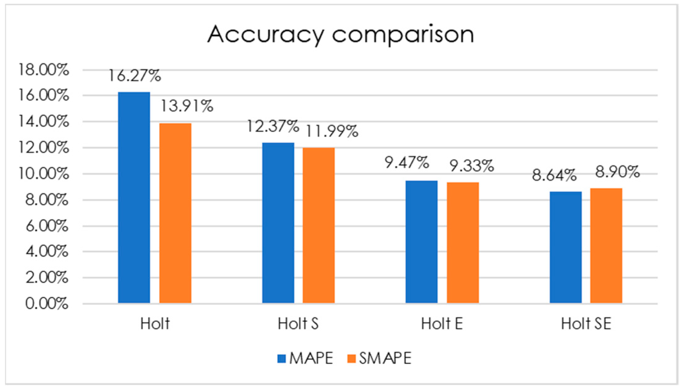
Similar to FE in Table 2, the final forecasts from all other methods can be obtained.

Table 4. Accuracy comparison.

Method	MAPE	SMAPE
Holt	16.27%	13.91%
Holt S	12.37%	11.99%
Holt E	9.47%	9.33%
Holt SE	8.64%	8.90%

summarizes and compares MAPEs and SMAPEs of the typical Holt’s method, denoted by Holt, with the three modified Holt’s method, i.e., Holt’s with seasonality, Holt’s with events, and Holt’s with seasonality and events, denoted by Holt S, Holt E, and Holt SE, respectively. Both MAPEs and SMAPEs of all four methods are also visualized by bar chart in Figure 3.

According to Table 4 and Figure 3, among all four methods, Holt performs the worst forecast on Thailand car sales data covering the COVID-19 pandemic period, in terms of both accuracy measures, possessing the highest MAPE and SMAPE at 16.27% and 13.91%, respectively. An improvement from Holt can be observed with the seasonality addressed in Holt S with lower MAPE and SMAPE at 12.37% and 11.99%. An even higher improvement from Holt can be obtained through Holt E, implying that, in the pandemic case, the event effects are stronger on these car sales data than the seasonal effects. Furthermore, the method combining both seasonal and event effects, Holt SE, achieving the lowest MAPE and SMAPE at 8.64% and 8.90%, respectively, indicates that this proposed modified Holt’s method best fits Thailand car sales data during the COVID-19 pandemic.

5. Conclusions

This study aimed to modify the typical Holt’s forecasting method to better suit time series data containing the event component, defined here as unusual impacts for a certain time period, largely caused by irregular incidents or events, such as the COVID-19 global pandemic.

As previously mentioned in the literature review section, there were previous attempts on capturing the effects of such irregular incidents into some forecasting models. More precisely, one attempt works with the regression method [10], while another works with the time-series decomposition (TSD) method [15]. The events of their interest are the2011 Thailand flood, along with the government’s tax-incentive program. Notably, their methods are completely different from what is proposed here because, unlike Holt’s method, both regression and TSD formulas are not recursive, nor need any smoothing constants.

Regardless, besides the typical Holt’s method, three modified methods based on Holt’s method including the seasonal and/or event components are proposed and named accordingly as the Holt’s method with seasonality, the Holt’s method with events, and the Holt’s method with seasonality and events. The methods with events incorporate another smoothing constant for the event estimate, denoted by δ and 0 ≤ δ ≤ 1. As for the methods with seasonality, the actual sales data are first de-seasonalized prior to being dealt with in the next steps.

All these four methods are implemented on Thailand’s monthly car sales data from January 2015 to December 2021, which also include the COVID-19 pandemic period. The input data obtained from the Office of Industrial Economics, Ministry of Industry, Thailand are flagged with different numbers to refer to various stages of the time period affected by the event of interest, i.e., the pandemic.

In terms of forecasting accuracy, the experimental results show that the Holt’s method with seasonality and events best fits the Thailand’s car sales data, possessing the lowest MAPE and SMAPE, among all the four methods. It must be noted that even the Holt’s method with events alone can also yield second best accuracy, much better than those of the typical Holt’s and the Holt’s with seasonality methods.

Beyond that, the modified Holt’s methods proposed in this research can certainly be applied to time series forecasting for other data largely impacted by abnormal events other than the COVID-19 pandemic. As evidenced here, the incorporation of another constant for the event estimate into Holt’s method significantly improves the forecasting accuracy; thus, the forecasted results can be used further in all kinds of planning for the business to stay competitive and beyond.

Last but not least, it would be interesting to compare the proposed methods with other time-series models. However, to ensure a fair comparison, a subtle way to incorporate the event component into the model of choice is, most likely, mandatory, and this is currently an ongoing project.

References

- ASEAN Briefing. Available online: https://www.aseanbriefing.com/news/thailands-automotive-industry-opportunities-incentives/ (accessed on 29 April 2022).
- CNN BUSINESS. Available online: https://money.cnn.com/2017/02/20/autos/traffic-rush-hour-cities/index.html (accessed on 29 April 2022).
- Mashable. Available online: https://mashable.com/article/bangkok-traffic-jams (accessed on 29 April 2022).
- Focus2move. Available online: https://www.focus2move.com/thailand-best-selling-car/#:~:text=Thailand%27s%20best%2Dselling%20car%20ranking,units%20sold%20(%2D4.8%25) (accessed on 29 April 2022).
- World Health Organization. Available online: https://www.who.int/emergencies/disease-outbreak-news/item/2020-DON234 (accessed on 28 April 2022).
- World Health Organization. Available online: https://www.who.int/news/item/13-10-2020-impact-of-covid-19-on-people’s-livelihoods-their-health-and-our-food-systems (accessed on 28 April 2022).
- The World Bank. Available online: https://www.worldbank.org/en/country/thailand/publication/monitoring-the-impact-of-covid-19-in-thailand#:~:text=Income%3A,income%20groups%20experiencing%20income%20%20declines (accessed on 28 April 2022).
- Leenawong, C. Logistics Intelligence and Forecasting with Excel 365; KMITL: Bangkok, Thailand, 2022; pp. 89–90. [Google Scholar]
- Wirotcheewan, P.; Kengpol, A.; Ishii, K.; Shimada, Y. Modelling and Forecasting for Automotive Parts Demand of Foreign Markets on Thailand. Asian Int. J. Sci. Technol. Prod. Manuf. Eng. 2011, 4, 1–13. [Google Scholar]
- Rattanametawee, W.; Leenawong, C.; Netisopakul, P. The Effects of Special Events on Regression for Subcompact Car Sales in Thailand. J. Teknol. 2016, 78, 161–165. [Google Scholar] [CrossRef] [Green Version]
- Booranawong, T.; Booranawong, A. Double exponential smoothing and Holt-Winters methods with optimal initial values and weighting factors for forecasting lime, Thai chili and lemongrass prices in Thailand. Eng. Appl. Sci. Res. 2018, 45, 32–38. [Google Scholar] [CrossRef]
- Muchayan, A. Comparison of Holt and Brown’s Double Exponential Smoothing Methods in The Forecast of Moving Price for Mutual Funds. J. Appl. Sci. Eng. Technol. Educ. 2019, 1, 183–192. [Google Scholar] [CrossRef]
- Sharif, O.; Hasan, M.Z. Forecasting the Stock Price by using Holt’s Method. Indones. J. Contemp. Manag. Res. 2019, 1, 15–24. [Google Scholar] [CrossRef]
- Suppalakpanya, K.; Nikhom, R.; Booranawong, T.; Booranawong, A. Study of Several Exponential Smoothing Methods for Forecasting Crude Palm Oil Productions in Thailand. Curr. Appl. Sci. Technol. 2019, 19, 123–149. [Google Scholar] [CrossRef]
- Rattanametawee, W.; Leenawong, C. Event Index Computation for Forecasting Case Study: Car Sales in Thailand. Thai J. Math. 2020, 18, 2079–2091. [Google Scholar]
- The Office of Industrial Economics, Ministry of Industry, Thailand. Available online: https://indexes.oie.go.th/industrialStatistics1.aspx (accessed on 3 August 2021).
- Leenawong, C. Data Analytics with Excel for Logistics & Supply Chain Management; CU Press: Bangkok, Thailand, 2022; p. 47. [Google Scholar]
- NIST. Available online: https://www.itl.nist.gov/div898/handbook/ (accessed on 6 February 2022).
- Hyndman, R.J.; Athanasopoulos, G. Forecasting: Principles and Practice, 2nd ed.; OTexts: Melbourne, Australia, 2018; p. 2. [Google Scholar]
Figure 1.
Thailand’s monthly car sales from January 2015 to December 2021.
Figure 2.
Thailand’s monthly car sales from January 2015 to December 2019 with a trendline.
Figure 3.
Bar chart of the forecasting accuracy.