The Effects of Pandemic Event on the Stock Exchange of Thailand

National Institute of Development Administration, NIDA Business School, Bangkok 10240, Thailand
Economies 2020, 8(4), 90; https://doi.org/10.3390/economies8040090
Submission received: 16 September 2020
/
Revised: 3 October 2020
/
Accepted: 6 October 2020
/
Published: 23 October 2020
Abstract
:The unprecedented global pandemic of COVID-19 has greatly impacted the stock market in terms of both price reactions and the influences of volatility. Using a sample of 46 stocks listed in the Stock Exchange of Thailand, in this paper, an event study technique is developed considering idiosyncratic volatility to analyze the reactions of stock prices and market volatility in Thailand during the period of the pandemic. The empirical results suggest that most securities in the Thai stock market have been adversely affected by the pandemic, as reflected in the abnormal returns compared to the period before the COVID-19 outbreak. This is mainly attributable to the curtailed economic activities induced by the pandemic as well as policy responses such as social distancing, quarantine and temporary market shutdown. Nevertheless, stocks in different sectors have been shown to have varied in terms of price responses, as some businesses may have benefitted from the pandemic. In terms of market volatility, the cumulated abnormal volatility (CAV) calculated in the paper suggests that volatility in the Stock Exchange of Thailand (SET) was significantly higher during the event window of COVID-19.
1. Introduction
The ongoing global pandemic of severe acute respiratory syndrome—known as COVID-19 or coronavirus disease 2019—has created unprecedented social and economic disruption around the globe. The outbreak of coronavirus 2 (SAR CoV2) was initially identified in Wuhan, China in December 2019. The World Health Organization declared the COVID-19 epidemic a Public Health Emergency of International Concern (PHEIC) on 30 January 2020, and later a global pandemic on 11 March 2020. Since then, the outbreak has spread around the globe, with far-reaching consequences beyond the spread of the virus itself. In terms of health and epidemic concerns, more than 20.6 million cases of COVID-19 have been confirmed in 188 countries, resulting in more than 749,000 deaths as of 13 August 2020. Nevertheless, COVID-19 is far more than a health crisis, as it also affects global economies and societies at their cores. One significant impact from the pandemic is to business and financial attitudes, which has been reflected by several business shutdowns and financial market turmoil. Thus, in this paper, we aim to investigate how the equity market is reacting to the specific event of the global spread of COVID-19 using the event study technique to empirically measure the abnormal returns and volatilities associated with this catastrophic event. The study also contributes to the extensive literature by analyzing the magnitude of the impact of COVID-19 on the behavior of the stock market in Thailand. Moreover, the idiosyncratic price and volatility reactions across different stocks are also captured in this study under the assumption that the impact of the pandemic would be asymmetric depending on the business sector of each stock; that is, regardless of the exogenous nature of the catastrophic event, stocks in the Thai equity market are expected to have uneven impacts in terms of excess returns and abnormal stock volatilities.
2. Literature Review
An extensive set of previous work has developed a method for determining event-induced effects on the volatility of asset returns. Using the stochastic volatility framework proposed by Bollerslev (1986), the Generalized Autoregressive Conditional Heteroskedasticity (GARCH) model allows for empirical tests of abnormal volatilities during a specific studied event. According to Bollerslev (1986), the GARCH model is an extension of the Autoregressive Conditional Heteroskedastic (ARCH) process developed by Engle (1982), in which the conditional variance of economic and financial variables varies over time as a function of past error. With the extension of the standard time series and more flexible lag structure than the ARCH process, the GARCH model allows for a more parsimonious and better fit for volatility clustering. Several empirical studies have adopted the GARCH framework to draw implications regarding the effect of a specific event, whether related to corporate changes or natural causes, on the unsystematic volatility of asset returns. The study in Akgiray (1989) also presents supportive evidence on the use of GARCH model. By fitting several ARCH process comparing with the GARCH (p,q) model with the equally-weighted and value-weighted Center for Research in Security Prices (CRSP) indexes, Akgirav found that GARCH (1,1) provide the strongest data fitness and forecast accuracy. In this light, the GARCH framework is useful for determining the significance of event-driven unsystematic volatility on asset returns, as it provides an empirical tool to identify factors affecting risks to financial securities.
Several works have provided empirical evidence for volatility event studies. According to McWilliams and Siegel (1997) and Mackinlay (1997), the event study approach is conventionally based on efficient market hypothesis where new information entering the market and received by the investors as a result of unexpected event that consequently impact current and future asset prices. Hilliard and Savickas (2002) developed an approach to measure the effects of an event on idiosyncratic volatility using the market model GARCH (1,1) to estimate abnormal returns due to a spin-off announcement of the randomly selected securities and portfolios by the Center for Research in Security Prices (CRSPAccess97) Stock File. The study found that the corporate spin-off announcement affected the volatility of the parent company’s idiosyncratic assets returns. This approach was a further contribution to previous studies on the effects of events on the volatility of asset returns, which have been addressed by several authors with methods including the nonparametric significance test for the estimation of abnormal returns, as introduced by Corrado (1989), and a parametric statistical test for abnormal asset returns associated with event-induced volatility, as developed by Boehmer et al. (1991).
An extensive set of empirical works has adopted event study methodology to analyze the effects of a shock on asset prices. Regarding price reactions and stock market volatility as a response to market shock, the study of Ruiz and Barrero (2014) adopted an event-study framework to estimate the impact of the 2010 Chilean natural disaster on the stock market. The empirical results suggested varying responses of abnormal returns and increases in stock market volatilities influenced by the earthquake shocks, where stocks in specific sectors—i.e., retail, construction and banking—experienced significant positive returns. Similarly, using the GARCH models, Wang and Kutan (2013) studied how natural disasters in Japan and the United States affect stocks in the insurance sector. Considering both the wealth and risk effects of natural disasters, the paper found that the stock markets of the US and Japan are well-diversified, reflected by the absence of wealth effects induced by the event. Nevertheless, significant wealth effects in these markets’ insurance sectors were empirically proven, indicating that wealth was redistributed between these two markets. On the contrary, Worthington (2008) used the GARCH-M (1,1) methodology to analyze the distributional and time-series effects of equity returns in the Australian equity market caused by natural events and disasters. The empirical findings of the study were quite noteworthy as they suggested no significant impact of natural events and disasters on the stock returns. This was due to the fact that the impact of natural events was diversified at the aggregate market level. Additionally, the drastic events were not systematically priced market factors, as the impact of the events was specific in terms of companies and/or regional areas. As such, the natural events observed in the paper were more unsystematic or represented non-market risks.
Lastly, a number of recent studies aim to explore economic impact of the unprecedented COVID-19 pandemic. Ramelli and Wagner (2020) provides cross-sectional reactions to COVID-19 in the U.S. stock market using the Russell 3000 index. The paper found that strong evidence for the role of international trade and global value chains on company value, especially with China exposure. That is, investors perceived companies in the U.S. more favorably when the COVID-19 situation in China improved relatively in Europe and in the United States. Davis et al. (2020) investigated how market shocks interacted to news about COVID-19 using the Risk Factors texts in 10-K filings of U.S. companies. The text-based model in the study suggested that bad news triggered significant negative abnormal return for firms with high exposures to COVID-19 such as travel and lodging sectors. Likewise, Baker et al. (2020) also found that impacts of the U.S. stock market were historically unprecedented with the pandemic-related daily stock movements being more severe compared to the Spanish Flu of 1918–1919 and the influenza pandemic of 1957–1958.
3. DATA and Methodology
The data used in the paper were the daily close prices of stocks traded in the Stock Exchange of Thailand (SET) for the period from 3 January 2019 to 1 April 2020. The calculation consisted of the top 50 stocks traded in the SET, whose rankings were based on large market capitalization, high liquidity and compliance with the requirements of share distribution to minor shareholders. Further, out of the so-called SET50 stocks, 46 companies were chosen by filtering out any stocks with less than 275 daily returns in the estimation period and those with missing values in the event window. In addition, the SET50 price index was also employed in the calculation as a proxy for the market index.
The returns were computed in logarithms of the stock prices and adjusted by dividends using the method applied by Fama (1965):
where
= the daily stock return of stock i at time t;
= the daily close price of stock i at time t;
= the dividend per share of stock i;
= the daily close price of stock i at time t − 1.
In addition, the volatility term was derived as follows:
Note that is the –algebra generated by ; theoretically, the volatility of the process should change over time.
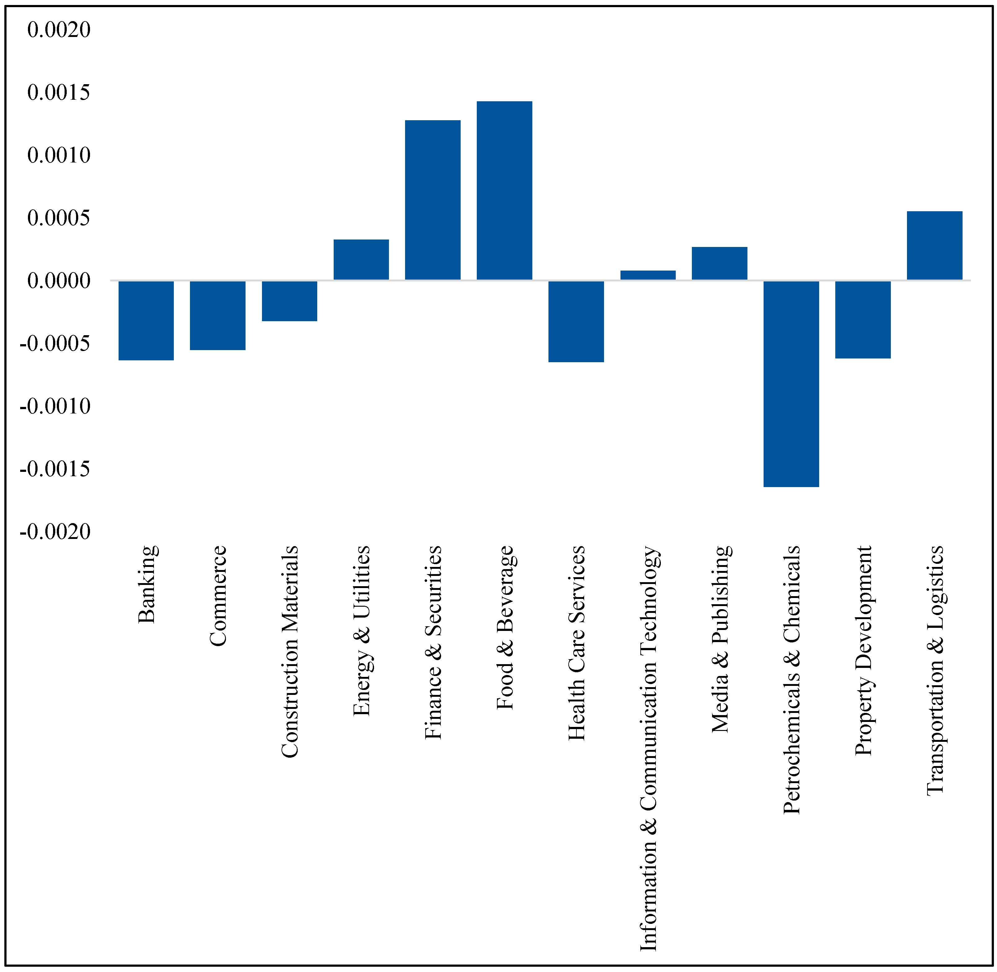
In order to check the properties of independent variables, the normality test was used to determine how likely it was for a random variable of the data set to be normally distributed. Table 1 shows the statistical summary of the daily returns of the sample which had an approximately symmetric distribution. Figure 1 shows the data denotes the estimation period consisting of 275 observations for each company.
4. Methodology
The main objective of this study was to investigate whether the unprecedented pandemic of COVID-19 has influenced volatility in the Thai stock market. The methodology used in the paper was based on the hypothesis of efficient markets suggested by Bromiley et al. (1988) and Fama et al. (1969), which implies that as soon as new financially relevant information enters the market and is absorbed by investors, the relevant information or market shocks will instantaneously be translated into stock prices. That is, asset prices are deemed to have an instant reaction to any new information revealed in the market. This hypothesis allows us to measure the impacts of a particular event over a period—i.e., a day—in which new relevant information enters the market. This observation period is thus known as the event window.
The conventional approach for an event study involves the specification of a market model for each firm in the observation. This assumes that as soon as the event conveys newly relevant information to the stock market, the mean or variance of abnormal returns must reflect the new economic conditions.
The simplest and most often used GARCH (1,1) process, commonly known as the generic vanilla GARCH model, is used to separate the systematic and unsystematic components of volatility. The method is as follows:
where
= rate of return on the stock price of firm i on day t;
= rate of return on a market portfolio of stock (i.e., SET50 price index) on day t;
= intercept term of firm i;
= systematic risk of stock of firm i;
= error term with E = 0;
= conditional variance, where the constant is the long-term average volatility, which must be greater than 0 (, and and ≥ 0 represent how the volatility is affected by current and past information regarding volatility, respectively.
Thus, if the stationary condition for GARCH (1,1), regarding , is satisfied, it means that the condition variance is finite.
The estimation of the daily abnormal conditional return (AR) which represents firm i in period t is based on the following equation:
where
= the set of conditional information in period t;
= the expected return from the actual return over an estimation period t preceding the event.
The abnormal returns represent the rate of returns earned by the firm after the analyst has adjusted for the “normal” return process, meaning that any significant difference is considered to be an abnormal return. Consequently, the test to measure the statistical significance following Dodd and Warner (1983) is
with
where
= the residual variance from the market model of firm i;
= the mean return on the market portfolio during the estimation period;
= the number of days in the estimation period.
In order to analyze the effect of COVID-19 during the event window, , the standardized cumulative abnormal return for each firm is calculated as
With the standard assumption that the value of is independent and identically distributed, the corresponding added statistical test to convert these values to identically distributed variables for security sample is
The next step, according to Hilliard and Savickas (2002), is to measure the effect of events on the unsystematic volatility of stock returns (). The estimation of for day t can be obtained by calculating the cross-sectional variance of the GARCH (1,1) residual. If the event does not affect the securities’ abnormal volatilities on day t, the should be equal to 1 (Bialkowski et al. 2006; Boehmer et al. 1991). If < 1, this implies that the event causes a decrease in volatility. Consequently, the event is characterized by a set of , which is required to calculate abnormal volatility.
The estimator of the cumulative abnormal volatility (CAV) between event days and is the sum of the individual estimators:
The null hypothesis regarding the effect of an event on the volatility of returns on day t is that there is no effect, which is expressed as
Then, the statistic test for the hypothesis is
The null hypothesis regarding the cumulative abnormal volatility is
Therefore, the statistic test for the hypothesis is
5. Empirical Results
The simulation results of the 46 portfolios in the observation period—covering the data of 12,650 securities—are discussed in this part. In order to analyze how the COVID-19 pandemic has affected the Thai stock market, the day of the event must first be defined. It is noteworthy that the subject of this work is unlike the previous event study literature, which relates to events with a narrow event window; i.e., natural disasters that occur exogenously but end in a much shorter time compared with the outbreak of coronavirus 2. In other words, in other event studies, the event window can be distinctly defined as it occurs and ends within a specific time period.
In contrast, given the fact that the COVID-19 pandemic is still an on-going event with a growing number of infected patients, the event window or observation period is less definite compared to other event study literature. In this study, the day of the event is defined as the day that the World Health Organization (WHO) declared COVID-19 a global pandemic—11 March 2020.
Empirical results are structured as follows: (i) Table 2 illustrates the post-COVID-19 standardized abnormal return of stocks in each sector obtained with GARCH (1,1); (ii) Table 3 provides an alternative approach to determining the cross-sectional differences of the impact of COVID-19 using market-adjusted abnormal returns; (iii) Table 4 and Table 5 show the pre-COVID-19 abnormal returns of stocks in the SET using the GARCH (1,1) process and alternative market-adjusted measures, respectively; (iv) Table 6 and Table 7 show descriptive statistics and abnormal t-tests with the GARCH (1,1) model of post and pre-COVID-19 event windows, respectively; and (v) descriptive statistics and abnormal return t-tests obtained by comparing individual firms’ returns with the market returns during pre and post-COVID-19 periods are presented in Table 8 and Table 9, respectively.
The empirical results suggest that most securities in the Stock Exchange of Thailand have abnormal negative returns during the observed period of the pandemic. This is mainly attributed to the worsened market sentiment induced by concerns over COVID-19 as well as curtailed economic activities as a result of policy responses to the pandemic such as social distancing, quarantine and market shutdown. Apparently, stocks in the Banking and Finance and Securities sectors are some of the most negative affected by the COVID-19 pandemic. According to Table 2, banks generally have a negative absolute return from the COVID-19 outbreak. This is because the pandemic has largely worsened the financial position of the private sector; i.e., the business and household sectors, who are the main customers of the banking sector. Furthermore, some banks have been shown to have statistically significant worsened abnormal returns. These include BBL (Bangkok Bank), KBANK (Kasikorn Bank) and TCAP (Thanachart Capital) with statistically significant post-COVID-19 abnormal returns in the periods observed. The findings are quite noteworthy given that the customer bases of BBL and KBANK are both corporate—BBL is well-known for its large corporation base—while KBANK targets more small and medium enterprises (SMEs). Moreover, in the finance and securities sector, SAWAD (Srisawad Corporation) has been the most negatively affected by the pandemic. This is due to the fact that the customer bases of SAWAD as well as TCAP in the banking sector are more concentrated on retail customers. Such a linkage between a customer portfolio that relies on the private sector—namely, businesses and households—and negative abnormal returns shows that the pandemic has indeed worsened the financial health of the private sector and the banking sector as a consequence.
Other than banking sector, several sectors have also been affected by the limited economic activities as a result of the outbreak. Firstly, the energy and utilities sector has been adversely affected by energy prices, especially oil and its related products. This is particularly due to the dramatic decrease in global demand induced by economic lockdown as a policy to deal with the pandemic in areas such as travel restrictions. This is reflected by the negative abnormal returns for oil companies in the SET such as PTT (Petroleum Authority of Thailand), PTTEP (PTT Exploration and Production) and EA (Energy Absolute). Moreover, according to the reduction in economic activities, companies in infrastructure services such as BGRIM (BGRIM Power), which is mainly involved in electricity production and sales, and TTW, which is the producer and provider of the water supply, have also exhibited significant negative abnormal returns during the pandemic period. Next, the food and beverage sector has also been notably affected by COVID-19, with the most apparent effect seen in MINT (Minor International), which is a business operator in food, beverages, hotels and rental services in department stores. This is due to the downturn in the tourism industry as a result of the travel restrictions as well as the temporary shutdown of department stores, markets and other tourism-related services. Lastly, according to the quarantine mandate induced by the pandemic, the transportation and logistics sector is another industry that has suffered adverse effects from the lower traffic and business activities, with the most negatively affected company being BEM (Bangkok Expressway and Metro), which mainly engages in the construction and operation of the Expressway and Operation Management of Mass Rapid Transit System Business (MRT).
Nevertheless, on the other side of the coin, there are some businesses that have benefitted from the pandemic as well. Despite statistical insignificance, BJC (Berli Jucker) and CPALL in the commerce sector have experienced a positive side of the influences of COVID-19. For BJC, the positive abnormal returns have been due to its business in the healthcare and technical supply chain, mainly in the distribution of pharmaceutical products and services. Likewise, CPALL, which is the owner of a ubiquitous convenience store—namely, 7-eleven—is another company that has benefitted from the pandemic, as its business has been excluded from the temporary business shutdown in policy responses to COVID-19.
In attempts to further develop our understanding of the cross-sectional dispersion of abnormal returns, an alternative measurement has been adopted using a market-adjusted approach. That is, abnormal returns for individual firms have been calculated as the differences between the return of each firm at time t and the market return in the same time period. With this approach, cross-sectional patterns of event-induced abnormal returns have been better captured, with the implications being the asymmetric effects of the pandemic on stock in different sectors. The empirical results in Table 3 emphasize the similar patterns of the cross-sectional impacts of COVID-19 on the Thai equity market as suggested by the results obtained through GARCH (1,1). However, there are some noteworthy differences: sectoral impacts are drawn more clearly when adjusted with the overall market returns instead of by processing with GARCH (1,1). That is, not only companies in the commerce sector—particularly BJC, CPALL and HMPRO—as suggested by the GARCH (1,1) process but also in the construction materials sector show abnormal returns due to the pandemic when adjusted with the market returns. In addition, a wider range of companies in different sectors exhibit negative impacts in terms of price returns than those obtained from the GARCH (1,1) process. These included—based on their overall statistical significance—(i) KBANK and TMB in the banking sector, (ii) MINT and TU in the food and beverage sector and (iii) ADVANC in information and communication technology.
The idiosyncratic pattern of abnormal returns induced by COVID-19 in the Thai equity market has been empirically proven using the GARCH specification as well as the market-adjusted returns of cross-sectional stocks by comparing the post-COVID-19 results with the pre-COVID-19 abnormal returns, as presented in Table 4 and Table 5, respectively. Note that the event window in the pre-COVID-19 specification was determined as the same event day in the previous year (11 March 2019). With the same sub-periods as in the previous exercises, it can be broadly seen that abnormal returns were more random across industries compared to those results induced by the pandemic.
Table 10 presents the cumulated abnormal volatility (CAV) calculated using asymmetric and symmetric window events as shown in the time interval (k,p); that is, the CAV values centered on the day of the event (11 March 2020)—CAV (0,5) and CAV (0,10)—are valued at −3.35 and 21.96, respectively. Based on the empirical findings in this paper, the CAV with statistical significance is within the 10-day window surrounding the event day when the WHO declared COVID-19 to be a global pandemic. It is found that the market volatility in the Stock Exchange of Thailand (SET) was 21.96% higher than in the same window if no pandemic had occurred. However, the empirical results in this study showed mixed signs of CAV as the event window changes despite the statistical insignificance of results other than CAV (0,10). This is possibly due to the fact that the pandemic is an on-going event, and thus the event window—stating a specific time in which an event has occurred and ended—cannot be accurately identified. Moreover, the event window is largely sensitive to the chosen day of the event; that is, the empirical results of the event study may provide different implications in accordance with the chosen day of the event as well as the time period in the event window.
6. Conclusions
In this paper, we adopted the event study technique to analyze the stock price reactions and market volatilities in response to the unprecedented global pandemic of COVID-19. Using the GARCH specification and event study methodology, the study empirically measures the abnormal returns and abnormal volatilities in the Stock Exchange of Thailand during the event window of the pandemic. In addition, the empirical framework used in this study also considered the idiosyncratic nature of prices and the volatility of stocks in different business sectors.
As a result, the findings suggest that the majority of stocks in the SET have been adversely influenced by the pandemic, as reflected by the abnormal negative returns during the event window of COVID-19, compared to their normal condition without the pandemic. Specifically, stocks in the banking, finance and securities, energy and utilities, food and beverage and transportation and logistics sectors have suffered an apparent negative abnormal impact in terms of the magnitude of impacts and statistical significance of results. This is attributable to the reduced economic activities induced by the pandemic as well as policy responses that the government has triggered to contain the dispersion of the COVID-19, which have resulted in excessive negative returns in the stocks of the associated industries. On the contrary, given the cross-sectional differences and idiosyncratic nature of stocks in each sector, some stocks have been shown to have experienced positive returns due to the event. These included businesses in the commerce sector, particularly companies which are distributors of pharmaceutical products and services. In an attempt to obtain robust empirical evidence, the cross-sectional differences in abnormal returns have also been measured using the market adjustment concept; that is, event-induced abnormal asset returns have been alternatively defined as each stock’s return adjusted with the total market returns. The results using market-adjusted returns are broadly in line with those obtained through the GARCH (1,1) process. In terms of market volatility, the cumulated abnormal volatility (CAV) calculated in the paper suggests that, within the 10-day window of the event day, the volatility in the SET is 21.96% higher than the normal window period without the influences of a pandemic.
Funding
This research received no external funding.
Acknowledgments
The author would like to thank Praewpailin Wongsindhuwises and Tarathip Tangkanjanapas for their excellent assistance on this research
Conflicts of Interest
The authors declare no conflict of interest.
References
- Akgiray, Vedat. 1989. Conditional Heteroscedasticity in Time Series of Stock Returns: Evidence and Forecasts. The Journal of Business 62: 55–80. [Google Scholar] [CrossRef]
- Bialkowski, Jędrzej, Katrin Gottschalk, and Tomasz Piotr Wisniewski. 2006. Stock market volatility around national elections. Journal of Banking and Finance 32: 941–1953. [Google Scholar] [CrossRef] [Green Version]
- Boehmer, Ekkehart, Jim Masumeci, and Annette B. Poulsen. 1991. Event-study methodology under conditions of event-induced variance. Journal of Financial Economics 30: 253–72. [Google Scholar] [CrossRef]
- Bollerslev, Tim. 1986. Generalized autoregressive conditional heteroskedasticity. Journal of Econometrics 31: 307–27. [Google Scholar] [CrossRef] [Green Version]
- Bromiley, Philip, Michele Govekar, and Alfred Marcus. 1988. On using event-study methodology in strategic management research. Technovation 8: 25–42. [Google Scholar] [CrossRef]
- Corrado, Charles J. 1989. A nonparametric test for abnormal security-price performance in event studies. Journal of Financial Economics 23: 385–95. [Google Scholar] [CrossRef]
- Davis, Steven J., Stephen Hansen, and Cristhian Seminario. 2020. Firm-Level Risk Exposures and Stock Price Reactions to COVID-19. NBER Working Paper, 27867. [Google Scholar]
- Dodd, Peter, and Jerold B. Warner. 1983. On corporate governance: A study of proxy contests. Journal of Financial Economics 11: 401–38. [Google Scholar] [CrossRef]
- Engle, Robert F. 1982. Autoregressive Conditional Heteroscedasticity with Estimates of the Variance of United Kingdom Inflation. Econometrics 50: 987–1007. [Google Scholar] [CrossRef]
- Fama, Eugene F. 1965. The behavior of stock-market prices. Journal of Business 38: 34105. [Google Scholar] [CrossRef]
- Fama, Eugene F., Lawrence Fisher, Michael C. Jensen, and Richard Roll. 1969. The adjustment of stock prices to new information. International Economic Review 10: 1–21. [Google Scholar] [CrossRef]
- Hilliard, Jimmy E., and Robert Savickas. 2002. On the statistical significance of event effects on unsystematic volatility. Journal of Financial Research 25: 447–62. [Google Scholar] [CrossRef]
- Mackinlay, A. Craig. 1997. Event studies in economics and finance. Journal of Economic Literature 35: 13–39. [Google Scholar]
- McWilliams, Abagail, and Donald Siegel. 1997. Event studies in management research: Theoretical and empirical issues. Academy of Management Journal 40: 626–57. [Google Scholar]
- Ramelli, Stefano, and Alexander F. Wagner. 2020. Feverish stock price reactions to COVID-19. Swiss Finance Institute Research Paper, 20–12. [Google Scholar] [CrossRef]
- Ruiz, José Luis, and Marcelo Barrero. 2014. The effects of the 2010 Chilean natural disasters on the stock market. Estudios de Administración 21: 31–48. [Google Scholar] [CrossRef]
- Baker, Scott R., Nicholas Bloom, Steven J. Davis, Kyle J. Kost, Marco C. Sammon, and Tasaneeya Viratyosin. 2020. The unprecedented stock market impact of COVID-19. NBER Working Paper, 26945. [Google Scholar]
- Wang, Lin, and Ali M. Kutan. 2013. The impact of natural disasters on stock markets: Evidence from Japan and the US. Comparative Economic Studies 55: 672–86. [Google Scholar] [CrossRef]
- Worthington, Andrew C. 2008. The impact of natural events and disasters on the Australian stock market: A GARCH-M analysis of storms, floods, cyclones, earthquakes and bushfires. Global Business and Economics Review 10: 1–10. [Google Scholar] [CrossRef] [Green Version]
Figure 1.
The average daily stock return of 46 listed companies traded on the SET by sector. Note: The data denotes the estimation period consisting of 275 observations for each company. Source: Stock Exchange of Thailand (SET).
Figure 1.
The average daily stock return of 46 listed companies traded on the SET by sector. Note: The data denotes the estimation period consisting of 275 observations for each company. Source: Stock Exchange of Thailand (SET).


Table 1.
The daily stock return of 46 listed companies traded on the Stock Exchange of Thailand (SET) market: statistical summary.
Table 1.
The daily stock return of 46 listed companies traded on the Stock Exchange of Thailand (SET) market: statistical summary.
| Symbol | Mean | Std. Dev | Skewness | Kurtosis |
|---|---|---|---|---|
| Banking | ||||
| BBL | −0.0013 | 0.0128 | 0.5581 | 0.5814 |
| KBANK | −0.0010 | 0.0161 | 0.1280 | 0.3049 |
| KTB | −0.0007 | 0.0097 | 0.0214 | 0.1197 |
| SCB | −0.0010 | 0.0162 | 0.2111 | 0.8376 |
| TCAP | 0.0003 | 0.0150 | 0.0544 | 0.0326 |
| TISCO | 0.0009 | 0.0122 | 0.1555 | 0.4664 |
| TMB | −0.0017 | 0.0187 | 0.0115 | 0.3154 |
| Commerce | ||||
| BJC | −0.0009 | 0.0148 | 0.0007 | 0.0074 |
| CPALL | 0.0001 | 0.0118 | 0.0398 | 0.0258 |
| GLOBAL | −0.0011 | 0.0169 | 0.0017 | 0.0345 |
| HMPRO | −0.0002 | 0.0139 | 0.0848 | 0.0613 |
| Construction Materials | ||||
| SCC | −0.0007 | 0.0116 | 0.4549 | 0.0339 |
| TOA | 0.0000 | 0.0195 | 0.0213 | 0.0810 |
| Energy & Utilities | ||||
| BGRIM | 0.0024 | 0.0209 | 0.5306 | 0.7636 |
| BPP | −0.0015 | 0.0136 | 0.0496 | 0.3950 |
| EA | 0.0002 | 0.0198 | 0.3330 | 0.1936 |
| EGCO | 0.0007 | 0.0122 | 0.0176 | 0.1636 |
| GPSC | 0.0011 | 0.0228 | 0.3785 | 0.5033 |
| GULF | 0.0028 | 0.0193 | 0.1315 | 0.2000 |
| IRPC | −0.0025 | 0.0220 | 0.0337 | 0.3378 |
| PTT | −0.0002 | 0.0117 | 0.0003 | 0.0003 |
| PTTEP | 0.0004 | 0.0143 | 0.0010 | 0.0019 |
| RATCH | 0.0008 | 0.0140 | 0.1620 | 0.0165 |
| TOP | −0.0007 | 0.0203 | 0.0336 | 0.0839 |
| TTW | 0.0004 | 0.0106 | 0.6392 | 0.1499 |
| Finance & Securities | ||||
| KTC | 0.0010 | 0.0205 | 0.0610 | 0.0872 |
| MTC | 0.0008 | 0.0195 | 0.6806 | 0.4445 |
| SAWAD | 0.0020 | 0.0202 | 0.9633 | 0.6929 |
| Food & Beverage | ||||
| CBG | 0.0038 | 0.0255 | 0.3402 | 0.1213 |
| MINT | −0.0001 | 0.0158 | 0.1176 | 0.4786 |
| OSP | 0.0022 | 0.0190 | 0.0692 | 0.0649 |
| TU | −0.0001 | 0.0184 | 0.0185 | 0.0743 |
| Health Care Services | ||||
| BDMS | 0.0000 | 0.0142 | 0.2963 | 0.2721 |
| BH | −0.0013 | 0.0171 | 0.0281 | 0.0035 |
| Information & Communication Technology | ||||
| ADVANC | 0.0007 | 0.0145 | 0.9777 | 0.2832 |
| INTUCH | 0.0006 | 0.0156 | 0.3329 | 0.2904 |
| TRUE | −0.0011 | 0.0209 | 0.8327 | 0.0891 |
| Media & Publishing | ||||
| VGI | 0.0003 | 0.0177 | 0.3731 | 0.6390 |
| Petrochemicals & Chemicals | ||||
| IVL | −0.0020 | 0.0275 | 0.0598 | 0.1794 |
| PTTGC | −0.0013 | 0.0180 | 0.0016 | 0.0023 |
| Property Development | ||||
| CPN | −0.0008 | 0.0154 | 0.2349 | 0.2481 |
| LH | −0.0002 | 0.0119 | 0.0055 | 0.0607 |
| WHA | −0.0008 | 0.0152 | 0.0040 | 0.0130 |
| Transportation & Logistics | ||||
| AOT | 0.0002 | 0.0128 | 0.4639 | 0.0589 |
| BEM | 0.0004 | 0.0138 | 0.6600 | 0.0900 |
| BTS | 0.0011 | 0.0141 | 0.0384 | 0.2440 |
Table 2.
Post-COVID-19 abnormal return obtained through the Generalized Autoregressive Conditional Heteroskedasticity (GARCH) (1,1) model.
| Banking | Commerce | ||||||||||
|---|---|---|---|---|---|---|---|---|---|---|---|
| Date | BBL | KBANK | KTB | SCB | TCAP | TISCO | TMB | BJC | CPALL | GLOBAL | HMPRO |
| 0 | −1.4% | −1.1% | −0.2% | 1.3% | −1.6% | −4.2% | 3.5% | −1.2% | 0.5% | 1.7% | 1.8% |
| +1 | −10.8% | −9.6% | −13.4% | −8.1% | −16.2% | −11.0% | −17.4% | −15.3% | −4.9% | −16.6% | −15.0% |
| +2 | −4.5% ** | 0.4% | 7.4% | 2.9% | 1.3% | 4.1% | 0.7% | 7.3% | 1.7% | 6.5% | 3.8% |
| +3 | −6.5% ** | −8.0% ** | −9.5% | −3.7% | −10.2% | −4.2% | −16.3% | 5.3% | −0.9% | −4.5% | −6.2% |
| +4 | −4.5% *** | −1.6% ** | −0.5% | 2.5% | −10.7% ** | −6.3% | 6.5% | 6.1% | 1.1% | 2.6% | 1.6% |
| +5 | 1.7% ** | 1.9% ** | 2.5% | 2.1% | −1.6% ** | −1.4% | 4.9% | 8.7% | 2.8% | 2.5% | 2.4% |
| +6 | −5.1% *** | −0.4% ** | 1.0% | 2.9% | −0.8% ** | −5.7% | 3.5% | 7.1% | 1.1% | −0.2% | −4.9% |
| +7 | 9.0% | 7.6% | 8.5% | 8.0% | 4.5% | 8.5% | 7.0% | 9.5% | 1.2% | 9.3% | 8.6% |
| +8 | −10.5% ** | −15.6% | −6.7% | −8.0% | −12.2% ** | −7.7% | −12.8% | −11.2% | 0.7% | −13.4% | −14.6% |
| +9 | 3.2% ** | 0.1% | 3.0% | 4.2% | 1.6% ** | 2.3% | 5.1% | 9.2% | 2.8% | −13.5% | −2.1% |
| +10 | 0.9% ** | 3.5% | 2.8% | 5.6% | 0.7% ** | 3.8% | 7.5% | 9.8% | 2.2% | 4.7% | 13.9% |
| Construction Materials | Energy & Utilities | ||||||||||||
|---|---|---|---|---|---|---|---|---|---|---|---|---|---|
| SCC | TOA | BGRIM | BPP | EA | EGCO | GPSC | GULF | IRPC | PTT | PTTEP | RATCH | TOP | TTW |
| −0.9% | 2.1% | −14.2% | −0.9% | −4.9% | −1.7% | −5.0% | −8.6% | 1.9% | 3.6% | 3.2% | −0.6% | 7.2% | −1.8% |
| −11.1% | −8.3% | −11.1% ** | −6.9% | −11.0% | −14.0% | −7.9% | −11.7% | −2.2% | −8.5% | −17.5% | −14.4% | −8.3% | −6.4% |
| 1.8% | 1.9% | 8.1% | −0.8% | 2.1% | 6.5% | 7.8% | 6.0% | 2.4% | 6.8% | 10.9% | 5.1% | 10.4% | −3.6% ** |
| −6.1% | −0.9% | −6.2% | −11.6% | −6.4% ** | −10.5% | −7.2% | −5.7% | −5.4% | −5.0% | −11.7% | −6.0% | −11.0% | −8.8% ** |
| 1.9% | 4.0% | 0.3% | 3.1% | −1.8% ** | 0.6% | 9.0% | 4.0% | 4.9% | 0.5% | 0.8% | 4.6% | −2.3% | −3.1% ** |
| 0.8% | 2.3% | 4.6% | 6.8% | 2.4% ** | 6.4% | 9.8% | 6.7% | 5.8% | 3.4% | −0.5% | 1.3% | 1.7% | 2.1% ** |
| 0.8% | 3.9% | 5.1% | 3.0% | 7.1% | 6.7% | 14.4% | 9.1% | 4.8% | −1.4% | −2.4% | 9.6% | 0.8% | −3.1% ** |
| 13.6% | 6.6% | 12.8% | 9.7% | 12.3% | 9.7% | 18.6% | 14.9% | 10.9% | 14.8% | 15.0% | 14.2% | 12.5% | 6.4% |
| −10.3% | −2.5% | −14.4% | −10.5% | −14.9% | −10.8% | −10.0% | −8.3% | −9.2% | −6.4% | −11.8% | −7.3% | −7.8% | −6.5% |
| 1.5% | 3.9% ** | 3.0% | 3.0% | 5.4% | 5.5% | 7.1% | 5.6% | 5.3% | 7.7% | 7.7% | 4.3% | 8.0% | 0.4% |
| 8.0% | 5.3% ** | 4.1% | 7.4% | 2.9% | 9.4% | 10.1% | 5.9% | 7.4% | 8.8% | 12.3% | 11.3% | 10.8% | 7.9% |
| Finance & Securities | Food & Beverage | Health Care Services | Information & Communication Technology | |||||||||
|---|---|---|---|---|---|---|---|---|---|---|---|---|
| Date | KTC | MTC | SAWAD | CBG | MINT | OSP | TU | BDMS | BH | ADVANC | INTUCH | TRUE |
| 0 | −2.8% | −4.0% | −6.5% | −1.3% | 1.0% | −2.3% | 1.0% | −2.5% | 1.0% | −2.0% | 0.1% | 1.0% |
| +1 | −19.1% | −8.5% | −16.9% | −18.0% | −15.9% | −15.1% | −13.2% | −7.8% | −3.8% | −4.5% | −8.3% | −8.4% |
| +2 | 7.1% | 7.2% | 6.6% | 1.9% | 0.9% | 5.4% | 5.9% | 3.0% | 0.4% | 4.1% | 2.6% | 3.1% |
| +3 | −3.1% | −12.5% | −11.9% | −6.1% | −13.3% | −11.5% | −1.1% | −8.3% | −5.3% | −1.3% | −3.8% | −5.7% |
| +4 | −6.1% | −14.2% | −7.9% ** | 0.0% | −7.1% | 1.3% | 2.0% | 1.7% | 2.3% | 2.8% | 2.4% | 5.3% |
| +5 | 4.0% | 1.2% | −4.5% ** | 1.3% | −8.5% ** | 6.7% | 3.5% | 5.4% | 5.3% | 6.4% | 4.1% | 16.6% |
| +6 | 2.1% | −8.8% | −8.2% ** | 12.4% | −2.3% ** | 4.2% | 7.7% | −3.2% | 8.7% | 7.6% | 8.5% | 15.3% |
| +7 | 12.1% | 15.2% | 13.1% | 15.2% | 8.8% | 14.7% | −3.9% | 10.4% | 2.0% | 5.7% | 9.2% | 7.5% |
| +8 | −13.7% | −13.9% | −17.0% ** | −13.6% | −14.0% | −14.7% | 1.2% | −10.5% | −3.2% | −2.7% | −5.3% | −5.9% |
| +9 | −9.1% | −10.3% | −14.4% ** | −2.6% | −2.0% ** | 0.5% | 2.6% | 1.1% | 3.0% | 5.3% | 1.3% | 4.4% |
| +10 | 0.6% | 3.3% | 0.7% ** | 6.8% | 4.3% | 7.7% | 7.9% | 5.4% | 3.3% | 6.0% | 7.0% | 6.7% |
| Media & Publishing | Petrochemicals & Chemicals | Property Development | Transportation & Logistics | |||||
|---|---|---|---|---|---|---|---|---|
| VGI | IVL | PTTGC | CPN | LH | WHA | AOT | BEM | BTS |
| −2.6% | 1.7% | −0.7% | −0.7% | 0.3% | −3.3% | −0.4% | −4.4% ** | −2.6% |
| −7.0% | −18.0% | −12.3% | −11.3% | −13.3% | −20.0% | −12.6% | −13.3% ** | −10.2% |
| 4.7% | 3.6% | 4.9% | 3.5% | 3.9% | 5.1% | 7.9% | 1.5% ** | 2.9% |
| −5.7% | −12.9% | −10.5% | −11.5% | −6.6% | −2.0% | −11.0% | −10.8% ** | −12.0% |
| 0.9% | 3.5% | 3.4% | −2.5% | −0.2% | 5.3% | 0.2% | −5.8% | 1.6% |
| 6.1% | 1.1% | 0.5% | 6.5% | 1.3% | 3.4% | 0.2% | 2.5% | 3.3% |
| −0.9% | 1.1% | 0.9% | −8.1% | −1.0% | −1.0% | −3.0% | 1.0% | 2.2% |
| 15.4% | 15.1% | 14.8% | 2.1% | 6.4% | 11.7% | 14.4% | 12.8% | 8.4% |
| −8.8% | −13.6% | −9.9% | −14.2% | −11.2% | −13.2% | −11.6% | −11.6% | −9.0% |
| −3.6% | 3.5% | 4.1% | 4.6% | 1.3% | −1.2% | 2.8% | −0.5% | −1.4% |
| 3.3% | 7.8% | 9.7% | 15.2% | 5.3% | 3.4% | 5.7% | 8.1% | 5.6% |
Note: ***, and ** denote significant at the 1%, and 5% level, respectively.
Table 3.
Post-COVID-19 abnormal returns obtained by means of comparing the returns of firms at time t with the return of the market at time t.
| Banking | Commerce | ||||||||||
|---|---|---|---|---|---|---|---|---|---|---|---|
| Date | BBL | KBANK | KTB | SCB | TCAP | TISCO | TMB | BJC | CPALL | GLOBAL | HMPRO |
| 0 | 0.7% | 0.6% | 1.2% | 1.3% | −0.1% | −3.3% | 4.0% | −1.3% | 1.2% *** | 2.0% | 2.7% ** |
| +1 | 1.8% | 2.5% | −1.9% | 1.7% | −4.5% | 0.1% | −7.0% | −5.7% | 5.8% *** | −6.4% | −3.9% |
| +2 | −7.3% | −3.0% | 3.5% | −2.6% | −2.4% | −0.2% | −4.2% | 1.6% | −3.0% ** | 1.3% | −0.5% |
| +3 | 2.0% | −0.2% | −2.2% | 1.7% | −2.7% | 2.5% | −10.2% | 10.5% | 5.4% ** | 1.3% | 0.6% |
| +4 | −3.3% | −1.1% | −0.6% | 0.5% | −10.6% | −7.0% | 5.2% | 3.8% | 0.1% ** | 0.9% | 0.9% |
| +5 | 0.4% | 0.0% | 0.1% | −2.3% | −3.8% | −4.3% | 1.3% | 4.1% | −0.6% ** | −1.5% | −0.6% |
| +6 | −4.8% | −0.7% | 0.2% | 0.2% | −1.4% | −7.1% | 1.5% | 4.2% | −0.7% ** | −2.6% | −6.2% |
| +7 | 0.3% | −1.6% | −1.2% | −3.3% | −5.0% | −1.6% | −3.7% | −1.9% | −9.3% | −1.7% | −1.6% |
| +8 | 0.3% | −5.4% | 2.9% | −0.4% | −2.4% | 1.4% | −4.4% | −3.8% | 9.3% | −5.4% | −5.5% |
| +9 | 1.7% | −1.9% | 0.4% | −0.3% | −0.8% | −0.8% | 1.3% | 4.5% | −0.8% | −17.6% | −5.3% |
| +10 | −4.2% | −2.2% | −3.3% | −2.3% | −5.3% | −2.9% | 0.3% | 1.8% | −4.8% | −2.9% | 7.3% |
| Construction Materials | Energe & Utilities | |||||||||||||
|---|---|---|---|---|---|---|---|---|---|---|---|---|---|---|
| Date | SCC | TOA | BGRIM | BPP | EA | EGCO | GPSC | GULF | IRPC | PTT | PTTEP | RATCH | TOP | TTW |
| 0 | 1.0% | 2.0% ** | −12.3% | −0.3% | −3.4% | −1.0% | −6.8% | −8.6% | 2.0% | 4.6% | 4.4% | −0.2% | 6.9% | 0.5% |
| +1 | 1.3% | 1.3% ** | 1.2% | 3.7% | 0.7% | −3.3% | −0.6% | −2.1% | 7.7% | 2.6% | −6.1% | −4.1% | 0.9% | 6.5% ** |
| +2 | −1.2% | −3.8% | 4.9% | −5.6% | −1.5% | 1.9% | −0.1% | 0.4% | −3.0% | 2.5% | 6.9% | 0.0% | 4.3% | −6.1% |
| +3 | 2.1% | 4.2% ** | 1.9% | −5.4% | 1.2% | −4.1% | −4.6% | −0.6% | 0.1% | 1.8% | −4.6% | −0.1% | −6.2% | 0.0% |
| +4 | 2.8% | 1.7% ** | 0.9% | 1.9% | −1.6% | −0.4% | 4.2% | 1.7% | 3.0% | 0.0% | 0.5% | 3.1% | −5.0% | −1.7% |
| +5 | −0.7% | −2.3% | 2.9% | 3.3% | 0.2% | 3.1% | 2.7% | 2.1% | 1.6% | 0.5% | −3.2% | −2.5% | −3.2% | 1.2% |
| +6 | 0.9% | 1.0% | 5.0% | 1.1% | 6.6% | 5.0% | 9.0% | 6.2% | 2.2% | −2.7% | −3.4% | 7.4% | −2.5% | −2.5% |
| +7 | 4.7% | −4.8% | 3.7% | −0.9% | 2.8% | −0.7% | 5.1% | 3.4% | −0.3% | 4.7% | 5.1% | 3.4% | 0.7% | −2.0% |
| +8 | 0.3% | 4.9% | −4.0% | −2.0% | −5.0% | −2.1% | −5.2% | −1.0% | −1.5% | 2.7% | −2.5% | 0.8% | −0.8% | 4.6% |
| +9 | −0.2% | −0.8% | 1.1% | −0.7% | 3.1% | 2.0% | −0.2% | 0.9% | 0.9% | 4.6% | 4.9% | 0.3% | 2.9% | −0.7% |
| +10 | 2.7% | −2.8% | −1.3% | 0.3% | −3.0% | 2.5% | −0.2% | −2.1% | −0.4% | 2.2% | 5.9% | 3.9% | 2.4% | 3.1% |
| Financial Securities | Food & Beverage | Health Care Services | Information & Communication Technology | |||||||||
|---|---|---|---|---|---|---|---|---|---|---|---|---|
| Date | KTC | MTC | SAWAD | CBG | MINT | OSP | TU | BDMS | BH | TRUE | ADVANC | INTUCH |
| 0 | −1.6% | −3.2% | −3.9% | −0.4% | 2.0% | −1.1% | 2.7% | −1.2% | 2.0% | 0.1% | −1.5% | 0.5% |
| +1 | −7.7% | 2.2% | −3.7% | −7.1% | −4.9% | −3.8% | −1.2% | 3.6% | 7.3% | 0.0% | 6.0% | 2.0% |
| +2 | 3.0% | 2.7% | 4.3% | −2.6% | −3.5% | 1.3% | 2.5% | −1.0% | −3.8% | −3.8% | −0.7% | −2.5% |
| +3 | 4.0% | −6.1% | −2.9% | 0.4% | −6.6% | −4.5% | 6.7% | −1.2% | 1.5% | −1.8% | 4.8% | 2.1% |
| +4 | −6.4% | −15.2% | −6.2% | −0.9% | −7.7% | 0.9% | 2.5% | 1.5% | 1.8% | 1.7% | 1.5% | 0.9% |
| +5 | 1.3% | −2.1% | −5.2% | −1.9% | −11.5% | 4.0% | 1.6% | 2.9% | 2.4% | 10.8% | 2.8% ** | 0.3% |
| +6 | 1.1% | −10.4% | −7.2% | 10.8% | −3.7% | 3.2% | 7.4% ** | −4.1% | 7.4% | 11.1% | 5.6% ** | 6.3% |
| +7 | 2.3% | 4.8% | 4.9% | 4.9% | −1.4% ** | 4.9% | −13.1% | 0.6% | −8.1% | −5.1% | −5.0% | −1.6% |
| +8 | −4.3% | −5.2% | −5.6% | −4.8% | −5.0% ** | −5.4% | 11.3% | −1.1% | 5.9% | 0.1% | 5.7% ** | 2.8% |
| +9 | −11.9% | −13.8% | −15.2% | −6.0% | −5.2% ** | −2.4% | 0.5% | −1.6% | 0.0% | −1.6% | 1.5% ** | −2.7% |
| +10 | −5.7% | −3.7% | −3.9% | 0.0% | −2.4% *** | 1.3% | 2.2% | −0.9% | −3.3% | −2.5% | −1.2% | −0.5% |
| Media & Publishing | Petrochemicals & Chemicals | Transportation & Logistics | |||||||
|---|---|---|---|---|---|---|---|---|---|
| Date | VGI | IVL | PTTGC | CPN | LH | WHA | AOT | BEM | BTS |
| 0 | −2.4% | 2.4% | 0.3% | 0.2% | 1.4% | −2.4% | 0.8% | −2.5% | −1.6% |
| +1 | 3.1% | −7.2% | −1.0% | −0.4% | −2.1% | −9.1% | −1.3% | −1.1% | 0.8% |
| +2 | −0.6% | −1.0% | 0.8% | −0.9% | −0.2% | 0.6% | 3.8% | −1.7% | −1.5% |
| +3 | −0.1% | −6.4% | −3.5% | −4.9% | 0.4% | 4.6% | −3.9% | −2.7% | −5.3% |
| +4 | −0.8% | 2.7% | 3.0% | −3.3% | −0.6% | 4.6% | −0.1% | −5.1% | 0.9% |
| +5 | 2.0% | −2.0% | −2.3% | 3.3% | −1.5% | 0.3% | −2.5% | 0.8% | 0.3% |
| +6 | −3.3% | −0.4% | −0.2% | −9.7% | −2.1% | −2.5% | −4.0% | 0.9% | 0.7% |
| +7 | 4.4% | 4.7% | 4.8% | −8.2% | −3.6% | 1.4% | 4.6% | 3.7% | −1.7% |
| +8 | −0.9% | −4.7% | −0.6% | −5.4% | −1.9% | −4.3% | −2.3% | −1.3% | 0.0% |
| +9 | −7.9% | 0.1% | 1.2% | 1.3% | −1.6% | −4.5% | 0.0% | −2.4% | −4.6% |
| +10 | −4.3% | 0.9% | 3.2% | 8.4% | −1.2% | −3.3% | −0.7% | 2.6% | −1.1% |
Note: ***, and ** denote significant at the 1%, and 5% level, respectively.
Table 4.
Pre-COVID-19 abnormal returns obtained through GARCH (1,1).
| Banking | Commerce | |||||||||
|---|---|---|---|---|---|---|---|---|---|---|
| Date | BBL | KBANK | KTB | SCB | TCAP | TISCO | TMB | BJC | GLOBAL | HMPRO |
| 0 | 0.5% | −0.2% | −0.5% | −0.3% | 0.0% | 0.2% | 0.1% | −0.3% | 0.7% | 0.7% |
| +1 | 0.5% | 0.3% | −0.5% | −0.3% | −1.4% | 0.8% | −4.4% | 1.2% | 0.1% | 1.3% |
| +2 | 1.0% | −0.2% | 0.0% | 0.1% | 1.8% | 0.2% | 2.0% | 0.2% | 0.6% | 1.3% |
| +3 | −0.5% | 0.1% | 0.0% | 0.1% | −1.4% | 0.8% | −0.8% | −0.8% | 0.1% | −2.6% |
| +4 | −0.5% | −1.8% | 0.0% | 0.5% | 0.4% | −0.3% | −0.8% | −0.8% | −2.8% | 0.0% |
| +5 | 0.5% | 0.1% | −1.0% | 0.5% | 0.4% | −0.9% | −0.8% | −0.3% | 0.7% | −0.6% |
| +6 | 0.0% | 1.1% | 1.1% | 0.9% | 2.7% | −0.9% | 0.1% | 1.7% | 2.4% | 0.0% |
| +7 | −0.5% | 0.3% | −0.5% | −0.7% | −0.5% | 0.8% | 0.1% | −0.3% | −0.5% | −0.7% |
| +8 | 0.0% | 0.1% | 1.6% | 0.1% | 0.8% | 0.8% | −1.8% | 0.7% | 2.3% | 0.7% |
| +9 | 0.0% | 0.8% | 1.1% | 3.1% | −1.4% | −0.3% | 2.0% | 0.1% | 1.1% | 1.3% |
| +10 | −0.5% | −1.2% | −1.6% | −1.4% | −1.9% | −0.9% | −0.8% | −1.3% | −4.5% | −2.0% |
| Construction &Materials | Energy & Utilities | ||||||||||||
|---|---|---|---|---|---|---|---|---|---|---|---|---|---|
| Date | SCC | TOA | BGRIM | BPP | EA | EGCO | GPSC | GULF | IRPC | PTT | PTTEP | TOP | TTW |
| 0 | 0.4% | 0.1% | −1.0% | 0.1% | −0.5% | 0.7% | −3.2% | −0.6% | −1.6% | −0.3% | −0.2% | −2.0% | −1.6% ** |
| +1 | 0.4% | −0.6% | 2.5% | 0.5% | −0.5% | 2.9% | −1.1% | 0.2% | 0.1% | 0.2% | 0.7% | 1.2% | 0.0% ** |
| +2 | 0.8% | −1.4% | 1.6% | 0.5% | 2.6% | 0.7% | −0.8% | 2.1% | 0.9% | 1.2% | 0.6% | 0.5% | 0.0% ** |
| +3 | 0.4% | 0.8% | 0.7% | −0.4% | 0.0% | −0.4% | 1.8% | −0.6% | −0.8% | 0.7% | −0.6% | −1.3% | 1.6% |
| +4 | −0.8% | −0.7% | −1.8% | 0.5% | 0.0% | −1.5% | −1.2% | −0.6% | −0.8% | 0.7% | −1.0% | −0.6% | 0.0% |
| +5 | 0.0% | −0.6% ** | 0.7% | 0.1% | 0.1% | 0.7% | −2.5% | −0.3% | 0.1% | −0.8% | 1.1% | −0.6% | −0.8% |
| +6 | 0.4% | 0.9% | −0.1% | 1.0% | 1.0% | 1.7% | 1.0% | 0.2% | 0.9% | 1.8% | 1.9% | 2.3% | −0.8% |
| +7 | −0.8% | −3.0% ** | −1.0% | −0.8% | −0.5% | −0.1% | −0.3% | 0.2% | 0.1% | −0.3% | −0.2% | −0.3% | 0.8% |
| +8 | 0.0% | 0.9% | −0.1% | 0.5% | 1.0% | −0.1% | 0.5% | 1.6% | 0.1% | 0.2% | 2.2% | 2.9% | 1.6% |
| +9 | 1.7% | −0.7% ** | −0.1% | 0.5% | 0.4% | 1.4% | 1.0% | 0.2% | 1.8% | 1.2% | 2.1% | 0.4% | 0.0% |
| +10 | −0.4% | −0.7% ** | −0.1% | −1.3% | −2.1% | 1.0% | −1.2% | −1.7% | −2.5% | −1.9% | −1.8% | −2.0% | −3.3% |
| Finance & Securities | Food & Beverage | Health Care Services | Information & Communication Technology | ||||||||
|---|---|---|---|---|---|---|---|---|---|---|---|
| Date | MTC | SAWAD | CBG | CPF | MINT | TU | BDMS | BH | 1 | ADVANC | DTAC |
| 0 | −1.7% | 1.0% | 2.1% | −1.1% | −0.7% | −0.5% | 0.1% | −0.4% | 0.3% | −0.2% | 1.6% |
| +1 | 1.1% | 1.5% | 3.3% | −2.1% ** | 0.6% | 2.2% | 0.9% | 1.3% | −0.1% | 0.3% | 1.6% |
| +2 | 3.3% | 2.5% | −0.9% | 3.8% | 1.2% | 0.6% | 0.5% | −0.1% | 0.7% | 0.9% | 1.0% ** |
| +3 | −0.6% | 0.0% | −2.7% | −0.1% | 0.6% | 0.0% | −0.8% | −0.4% | −0.1% | −0.3% | −1.8% |
| +4 | −0.6% | −0.5% | 2.5% | 1.8% | −2.6% | −0.5% | −0.3% | −0.1% | −0.9% | 0.0% | 0.6% |
| +5 | 0.6% | 2.0% | −2.6% | −2.0% | −0.7% | −0.5% | 0.1% | −0.4% | −0.5% | 0.0% | −1.8% |
| +6 | 1.1% | 1.9% | 1.7% | −2.0% | 1.3% | −0.5% | −0.3% | 0.2% | 1.1% | 0.9% | −0.9% |
| +7 | 0.5% | 1.4% | 0.8% | −0.1% | 0.0% | 0.0% | 1.8% | −0.1% | −0.1% | 0.3% | −2.8% |
| +8 | 0.5% | 0.0% | −0.5% | 0.9% | 0.6% | 1.1% | 1.3% | 0.4% | 0.7% | 1.1% | 2.1% |
| +9 | −0.1% | −1.0% | −0.6% | 1.9% | 0.6% | 1.1% | 1.7% | 0.7% | 1.0% | 0.8% | 2.0% |
| +10 | −3.3% | −0.9% | −0.5% | −2.0% | −1.3% | −0.5% | −1.1% | −1.5% | −1.0% | −2.4% | −2.3% |
| Petrochemicals & Chemicals | Property Development | Transportation & Logistics | |||||
|---|---|---|---|---|---|---|---|
| Date | PTTGC | CPN | LH | WHA | AOT | BEM | BTS |
| 0 | −0.4% | −0.3% | 0.0% | −0.4% | 0.1% | −1.7% | 0.0% |
| +1 | 0.0% | −0.7% | 0.0% | 0.1% | −1.0% | 0.3% | 0.0% |
| +2 | 0.7% | 0.7% | 0.0% | 1.0% | 2.7% | 0.8% | 0.0% |
| +3 | 0.0% | −0.7% | 0.0% | 0.6% | 0.4% | −0.2% | 0.9% |
| +4 | 0.0% | −1.0% | −1.9% | −0.8% | −1.4% | −0.2% | −1.0% |
| +5 | 0.8% | −0.3% | 0.0% | 0.1% | −1.4% | −0.2% | 0.0% |
| +6 | 1.1% | 1.1% | 0.0% | 0.6% | 1.2% | −0.2% | −1.0% |
| +7 | −1.1% | 0.7% | −0.9% | 0.1% | −0.3% | −1.2% | 0.9% |
| +8 | 1.4% | 0.4% | 0.0% | 1.0% | 0.4% | 0.8% | −1.9% |
| +9 | 1.7% | 0.0% | 3.8% | −0.4% | 0.8% | −0.1% | 2.7% |
| +10 | −1.5% | −0.3% | −0.9% | −0.4% | −0.7% | 0.8% | 0.0% |
Note: ** denote significant and 5% level, respectively.
Table 5.
Pre-COVID-19 abnormal returns obtained by means of comparing the returns of firms at time t with the return of the market at time t.
| Banking | Commerce | |||||||||
|---|---|---|---|---|---|---|---|---|---|---|
| Date | BBL | KBANK | KTB | SCB | TCAP | TISCO | TMB | BJC | GLOBAL | HMPRO |
| 0 | 0.7% | 0.0% | −0.3% | −0.1% | 0.3% | 0.5% ** | 0.3% | −0.2% | 0.8% | 0.9% |
| +1 | 0.5% | 0.3% | −0.5% | −0.4% | −1.4% | 0.8% *** | −4.6% | 1.0% | 0.0% | 1.3% |
| +2 | 0.1% | −1.1% | −0.9% | −0.9% | 0.9% | −0.6% ** | 1.0% | −0.9% | −0.3% | 0.4% |
| +3 | −0.3% | 0.2% | 0.2% | 0.2% | −1.2% | 1.0% ** | −0.7% | −0.8% | 0.2% | −2.4% |
| +4 | 0.2% | −1.2% | 0.7% | 1.0% | 1.1% | 0.4% *** | −0.3% | −0.3% | −2.2% | 0.7% |
| +5 | 1.0% | 0.5% | −0.6% | 0.9% | 1.0% | −0.3% ** | −0.4% | 0.0% | 1.1% | −0.2% |
| +6 | −0.9% | 0.2% | 0.2% | −0.1% | 1.8% | −1.7% | −0.9% | 0.6% | 1.4% | −0.9% |
| +7 | −0.3% | 0.5% | −0.3% | −0.5% | −0.2% | 1.1% | 0.2% | −0.3% | −0.4% | −0.4% |
| +8 | −0.5% | −0.5% | 1.1% | −0.5% | 0.4% | 0.3% | −2.4% | 0.0% | 1.8% | 0.2% |
| +9 | −1.0% | −0.3% | 0.0% | 2.0% | −2.4% | −1.3% | 0.9% | −1.0% | 0.1% | 0.3% |
| +10 | 1.0% | 0.1% | −0.1% | 0.0% | −0.4% | 0.6% | 0.5% | 0.0% | −3.1% | −0.5% |
| Construction Materials | Energy & Utilities | ||||||||||||
|---|---|---|---|---|---|---|---|---|---|---|---|---|---|
| Date | SCC | TOA | BGRIM | BPP | EA | EGCO | GPSC | GULF | IRPC | PTT | PTTEP | TOP | TTW |
| 0 | 0.7% | 0.3% | −0.6% | 0.3% | −0.3% | 1.0% | −3.1% | −0.3% | −1.5% | −0.3% | −0.2% | −1.9% | −1.4% |
| +1 | 0.4% | −0.8% | 2.6% | 0.4% | −0.5% | 2.9% | −1.3% | 0.3% | 0.0% | 0.0% | 0.4% | 1.1% | 0.0% |
| +2 | −0.1% | −2.4% ** | 0.8% | −0.4% | 1.7% | −0.2% | −1.8% | 1.3% | 0.0% | 0.2% | −0.5% | −0.5% | −0.9% |
| +3 | 0.6% | 0.9% ** | 1.0% | −0.3% | 0.2% | −0.2% | 1.9% | −0.4% | −0.7% | 0.7% | −0.6% | −1.2% | 1.8% |
| +4 | −0.2% | −0.1% ** | −1.0% | 1.1% | 0.7% | −0.8% | −0.6% | 0.1% | −0.2% | 1.2% | −0.6% | −0.1% | 0.7% |
| +5 | 0.5% | −0.3% ** | 1.3% | 0.5% | 0.5% | 1.2% | −2.1% | 0.2% | 0.5% | −0.5% | 1.3% | −0.2% | −0.3% |
| +6 | −0.5% | −0.1% ** | −0.9% | 0.0% | 0.1% | 0.9% | 0.0% | −0.6% | 0.0% | 0.7% | 0.8% | 1.3% | −1.7% |
| +7 | −0.6% | −2.9% ** | −0.6% | −0.7% | −0.3% | 0.2% | −0.2% | 0.5% | 0.2% | −0.3% | −0.2% | −0.1% | 1.0% |
| +8 | −0.5% | 0.3% ** | −0.5% | −0.1% | 0.5% | −0.5% | −0.1% | 1.1% | −0.5% | −0.5% | 1.5% | 2.3% | 1.1% |
| +9 | 0.6% | −1.8% *** | −1.0% | −0.6% | −0.5% | 0.4% | −0.2% | −0.8% | 0.7% | 0.0% | 0.9% | −0.7% | −1.0% |
| +10 | 1.0% | 0.7% ** | 1.4% | 0.1% | −0.6% | 2.5% | 0.1% | −0.2% | −1.1% | −0.6% | −0.5% | −0.7% | −1.8% |
| Finance & Securities | Food & Beverage | Health Care Services | Information & Communication Techonology | ||||||||
|---|---|---|---|---|---|---|---|---|---|---|---|
| Date | MTC | SAWAD | CBG | CPF | MINT | TU | BDMS | BH | TRUE | ADVANC | DTAC |
| 0 | −1.5% | 1.3% | 2.0% | −0.7% | −0.4% | −0.3% | 0.3% | −0.3% | 0.3% | 0.0% | 1.7% |
| +1 | 1.1% | 1.5% | 3.0% | −2.0% | 0.6% | 2.2% | 0.8% | 1.1% | −0.4% | 0.3% | 1.4% |
| +2 | 2.5% | 1.6% | −2.1% | 3.0% | 0.4% | −0.4% | −0.5% | −1.2% | −0.5% | −0.1% | 0.0% |
| +3 | −0.4% | 0.2% | −2.8% | 0.2% | 0.8% | 0.2% | −0.7% | −0.4% | −0.2% | −0.1% | −1.7% |
| +4 | 0.1% | 0.2% | 2.8% | 2.6% | −1.9% | 0.1% | 0.2% | 0.4% | −0.6% | 0.7% | 1.1% |
| +5 | 1.1% | 2.5% | −2.5% | −1.4% | −0.2% | 0.0% | 0.5% | −0.1% | −0.3% | 0.5% | −1.4% |
| +6 | 0.2% | 1.0% | 0.4% | −2.8% | 0.4% | −1.4% | −1.3% | −0.9% | −0.1% | −0.1% | −1.9% |
| +7 | 0.8% | 1.6% | 0.6% | 0.2% | 0.2% | 0.2% | 1.9% | −0.1% | −0.2% | 0.5% | −2.8% |
| +8 | 0.0% | −0.5% | −1.4% | 0.5% | 0.1% | 0.6% | 0.8% | −0.2% | −0.1% | 0.6% | 1.5% |
| +9 | −1.0% | −2.0% | −1.9% | 0.9% | −0.4% | 0.0% | 0.6% | −0.5% | −0.2% | −0.2% | 0.9% |
| +10 | −1.8% | 0.5% | 0.6% | −0.5% | 0.2% | 0.9% | 0.2% | −0.2% | 0.2% | −1.0% | −1.0% |
| Petrochemicals & Chemicals | Property Development | Transportation & Logistics | |||||
|---|---|---|---|---|---|---|---|
| Date | PTTGC | CPN | LH | WHA | AOT | BEM | BTS |
| 0 | −0.5% | −0.1% | 0.3% | −0.2% | 0.3% | −1.2% | 0.3% |
| +1 | −0.4% | −0.7% | 0.0% | 0.0% | −1.1% | 0.5% | 0.0% |
| +2 | −0.5% | −0.2% | −0.9% | 0.1% | 1.7% | 0.1% | −0.9% |
| +3 | −0.2% | −0.5% | 0.2% | 0.7% | 0.5% | 0.2% | 1.1% |
| +4 | 0.3% | −0.4% | −1.2% | −0.3% | −0.8% | 0.7% | −0.3% |
| +5 | 0.9% | 0.2% | 0.5% | 0.5% | −1.0% | 0.5% | 0.5% |
| +6 | −0.2% | 0.1% | −0.9% | −0.4% | 0.2% | −0.9% | −1.8% |
| +7 | −1.3% | 0.9% | −0.8% | 0.2% | −0.2% | −0.8% | 1.1% |
| +8 | 0.6% | −0.2% | −0.5% | 0.5% | −0.1% | 0.5% | −2.4% |
| +9 | 0.4% | −1.0% | 2.8% | −1.5% | −0.3% | −1.0% | 1.7% |
| +10 | −0.4% | 1.1% | 0.5% | 1.0% | 0.7% | 2.4% | 1.4% |
Note: ***, and ** denote significant at the 1%, and 5% level, respectively.
Table 6.
Post-COVID-19 descriptive statistics and abnormal returns t-test through GARCH (1,1).
| Day | MIN | AVERAGE | MAX | STD DEV | SKEWNESS | KURTOSIS | Prob>chi2 |
|---|---|---|---|---|---|---|---|
| 0 | −14.2% | −1.1% | 7.2% | 3.5% | 0.0017 | 0.0037 | 0.0008 *** |
| +1 | −20.0% | −11.6% | −2.2% | 4.4% | 0.9956 | 0.4305 | 0.7259 |
| +2 | −4.5% | 4.0% | 10.9% | 3.2% | 0.6355 | 0.9598 | 0.8926 |
| +3 | −16.3% | −7.3% | 5.3% | 4.2% | 0.7656 | 0.7930 | 0.9241 |
| +4 | −14.2% | 0.3% | 9.0% | 4.6% | 0.0001 | 0.0057 | 0.0002 *** |
| +5 | −8.5% | 3.2% | 16.6% | 3.8% | 0.2942 | 0.0026 | 0.0127 ** |
| +6 | −8.8% | 2.0% | 15.3% | 5.7% | 0.6274 | 0.6865 | 0.8164 |
| +7 | −3.9% | 10.1% | 18.6% | 4.5% | 0.0578 | 0.8561 | 0.1450 |
| +8 | −17.0% | −10.0% | 1.2% | 4.2% | 0.0065 | 0.2277 | 0.0204 ** |
| +9 | −14.4% | 1.6% | 9.2% | 5.1% | 0.0000 | 0.0059 | 0.0001 *** |
| +10 | 0.6% | 6.3% | 15.2% | 3.4% | 0.0490 | 0.6919 | 0.1237 |
Note: ***, and ** denote significant at the 1%, and 5% level, respectively. Source: Authors’ calculation based on Stock Exchange of Thailand (SET).
Table 7.
Pre-COVID-19 descriptive statistics and abnormal returns t-test through GARCH (1,1).
| Day | MIN | AVERAGE | MAX | STD DEV | SKEWNESS | KURTOSIS | Prob>chi2 |
|---|---|---|---|---|---|---|---|
| 0 | −3.2% | −0.3% | 2.1% | 1.0% | 0.5044 | 0.0371 | 0.0920 |
| +1 | −4.4% | 0.3% | 3.3% | 1.3% | 0.0508 | 0.0044 | 0.0070 *** |
| +2 | −1.4% | 0.9% | 3.8% | 1.1% | 0.0831 | 0.1500 | 0.0825 |
| +3 | −2.7% | −0.2% | 1.8% | 0.9% | 0.0482 | 0.0390 | 0.0263 ** |
| +4 | −2.8% | −0.5% | 2.5% | 1.0% | 0.5643 | 0.1934 | 0.3433 |
| +5 | −2.6% | −0.3% | 2.0% | 0.9% | 0.4123 | 0.1181 | 0.1911 |
| +6 | −2.0% | 0.7% | 2.7% | 1.0% | 0.0920 | 0.0130 | 0.0194 ** |
| +7 | −3.0% | −0.2% | 1.8% | 0.9% | 0.0057 | 0.0001 | 0.0002 *** |
| +8 | −1.9% | 0.7% | 2.9% | 0.9% | 0.5223 | 0.1608 | 0.2842 |
| +9 | −1.4% | 0.8% | 3.8% | 1.1% | 0.2020 | 0.3071 | 0.2425 |
| +10 | −4.5% | −1.3% | 1.0% | 1.0% | 0.9666 | 0.1700 | 0.3698 |
Note: ***, and ** denote significant at the 1%, and 5% level, respectively. Source: Authors’ calculation based on Stock Exchange of Thailand (SET).
Table 8.
Post-COVID-19 descriptive statistics and abnormal returns t-test obtained by comparing the returns of firms at time t with the return of the market at time t.
Table 8.
Post-COVID-19 descriptive statistics and abnormal returns t-test obtained by comparing the returns of firms at time t with the return of the market at time t.
| Date | Banking | Commerce | Construction | Energy & Utilities | Finance & Securities |
| 0 | 0.6% | 1.2% ** | 1.5% | −1.2% | −2.9% |
| +1 | −1.0% | −2.6% | 1.3% | 0.6% | −3.1% |
| +2 | −2.3% | −0.1% | −2.5% | 0.4% | 3.3% |
| +3 | −1.3% | 4.4% | 3.2% | −1.7% | −1.7% |
| +4 | −2.4% | 1.4% | 2.3% | 0.5% | −9.3% |
| +5 | −1.2% | 0.4% | −1.5% | 0.7% | −2.0% |
| +6 | −1.7% | −1.3% | 0.9% | 2.6% | −5.5% |
| +7 | −2.3% | −3.6% | −0.1% | 2.1% | 4.0% |
| +8 | −1.1% | −1.4% | 2.6% | −1.3% | −5.0% |
| +9 | −0.1% | −4.8% | −0.5% | 1.6% | −13.6% |
| +10 | −2.8% | 0.3% | −0.1% | 1.1% | −4.4% |
| Date | Food & Beverage | Health Care Services | Information & Communication Technology | ||
| 0 | 0.8% | 0.4% | −0.3% | ||
| +1 | −4.3% | 5.5% | 2.7% | ||
| +2 | −0.6% | −2.4% | −2.3% | ||
| +3 | −1.0% | 0.2% | 1.7% | ||
| +4 | −1.3% | 1.6% | 1.4% | ||
| +5 | −2.0% | 2.6% | 4.6% | ||
| +6 | 4.4% | 1.6% | 7.6% | ||
| +7 | −1.2% | −3.8% | −3.9% | ||
| +8 | −1.0% | 2.4% | 2.9% | ||
| +9 | −3.3% | −0.8% | −0.9% | ||
| +10 | 0.3% | −2.1% | −1.4% | ||
| Date | Media & Publishing | Petrochemicals & Chemicals | Property Development | Transportation & Logistics | |
| 0 | −2.4% | 1.4% | −0.3% | −1.1% | |
| +1 | 3.1% | −4.1% | −3.9% | −0.5% | |
| +2 | −0.6% | −0.1% | −0.2% | 0.2% | |
| +3 | −0.1% | −4.9% | 0.0% | −4.0% | |
| +4 | −0.8% | 2.8% | 0.2% | −1.4% | |
| +5 | 2.0% | −2.1% | 0.7% | −0.5% | |
| +6 | −3.3% | −0.3% | −4.8% | −0.8% | |
| +7 | 4.4% | 4.8% | −3.5% | 2.2% | |
| +8 | −0.9% | −2.7% | −3.8% | −1.2% | |
| +9 | −7.9% | 0.7% | −1.6% | −2.3% | |
| +10 | −4.3% | 2.1% | 1.3% | 0.3% | |
Note: ** denote significant at the and 5% level, respectively.
Table 9.
Pre-COVID-19 descriptive statistics and abnormal returns t-test obtained by comparing the returns of firms at time t with the return of the market at time t.
Table 9.
Pre-COVID-19 descriptive statistics and abnormal returns t-test obtained by comparing the returns of firms at time t with the return of the market at time t.
| Date | Banking | Commerce | Construction | Energy & Utilities | Finance & Securities |
|---|---|---|---|---|---|
| 0 | 0.2% | 0.5% | 0.5% | −0.7% | −0.1% |
| +1 | −0.8% | 0.8% | −0.2% | 0.5% | 1.3% |
| +2 | −0.2% | −0.3% | −1.2% | 0.0% | 2.0% |
| +3 | −0.1% | −1.0% | 0.8% | 0.2% | −0.1% |
| +4 | 0.3% | −0.6% | −0.1% | 0.0% | 0.1% |
| +5 | 0.3% | 0.3% | 0.1% | 0.2% | 1.8% |
| +6 | −0.2% | 0.4% | −0.3% | 0.0% | 0.6% |
| +7 | 0.1% | −0.4% | −1.8% | 0.0% | 1.2% |
| +8 | −0.3% | 0.6% | −0.1% | 0.4% | −0.2% |
| +9 | −0.3% | −0.2% | −0.6% | −0.3% | −1.5% |
| +10 | 0.2% | −1.2% | 0.8% | −0.1% | −0.7% |
| Date | Food & Beverage | Health Care Services | Information & Communication Technology | ||
| 0 | 0.1% | 0.0% | 0.6% | ||
| +1 | 0.9% | 1.0% | 0.4% | ||
| +2 | 0.2% | −0.8% | −0.2% | ||
| +3 | −0.4% | −0.5% | −0.7% | ||
| +4 | 0.9% | 0.3% | 0.4% | ||
| +5 | −1.0% | 0.2% | −0.4% | ||
| +6 | −0.9% | −1.1% | −0.7% | ||
| +7 | 0.3% | 0.9% | −0.8% | ||
| +8 | 0.0% | 0.3% | 0.7% | ||
| +9 | −0.4% | 0.1% | 0.2% | ||
| +10 | 0.3% | 0.0% | −0.6% | ||
| Date | Petrochemicals & Chemicals | Property Development | Transportation & Logistics | ||
| 0 | −0.5% | 0.0% | −0.2% | ||
| +1 | −0.4% | −0.2% | −0.2% | ||
| +2 | −0.5% | −0.3% | 0.3% | ||
| +3 | −0.2% | 0.1% | 0.6% | ||
| +4 | 0.3% | −0.6% | −0.1% | ||
| +5 | 0.9% | 0.4% | 0.0% | ||
| +6 | −0.2% | −0.4% | −0.8% | ||
| +7 | −1.3% | 0.1% | 0.1% | ||
| +8 | 0.6% | −0.1% | −0.7% | ||
| +9 | 0.4% | 0.1% | 0.1% | ||
| +10 | −0.4% | 0.9% | 1.5% | ||
Table 10.
Test results for cumulative abnormal volatility within sub-periods of the event window.
| Time Interval (m,s) | |||||
|---|---|---|---|---|---|
| (0,5) | (0,10) | (−5,5) | (−10,10) | (−15,15) | |
| −3.35 | 21.96 *** | 2.17 | 16.75 | −15.86 | |
Note: *** denote significant at the 1% level.
Publisher’s Note: MDPI stays neutral with regard to jurisdictional claims in published maps and institutional affiliations. |
© 2020 by the author. Licensee MDPI, Basel, Switzerland. This article is an open access article distributed under the terms and conditions of the Creative Commons Attribution (CC BY) license (http://creativecommons.org/licenses/by/4.0/).
Share and Cite
MDPI and ACS Style
Panyagometh, K. The Effects of Pandemic Event on the Stock Exchange of Thailand. Economies 2020, 8, 90. https://doi.org/10.3390/economies8040090
AMA Style
Panyagometh K. The Effects of Pandemic Event on the Stock Exchange of Thailand. Economies. 2020; 8(4):90. https://doi.org/10.3390/economies8040090
Chicago/Turabian StylePanyagometh, Kamphol. 2020. "The Effects of Pandemic Event on the Stock Exchange of Thailand" Economies 8, no. 4: 90. https://doi.org/10.3390/economies8040090
Note that from the first issue of 2016, this journal uses article numbers instead of page numbers. See further details here.