I. Introduction
In this paper, we examine the reaction of stock markets around the globe during both the global financial crisis (GFC) of 2007–2008 and the current COVID-19 pandemic. As a result of the crises, we expect to find increased market interconnectedness due to herding behavior. Herd behavior is a phenomenon where individuals act collectively, not using their own information. This behavior, described by Bikhchandani-Sharma (2000), is often observed in financial markets, especially during crises, when irrationality prevails. The negative news about the spread of COVID-19 and overall negative sentiment affected investor psychology and led to intense trading behavior in the market (for COVID-19 articles and summary, see Sharma & Sha, 2020).
Our hypothesis is that market connectedness has increased over time. We measure market activity by using both market returns and volatility. To test our hypothesis, we employ data for 19 countries and energy derivatives covering the 1992–2020 period and the spillover index based on vector autogression (VAR) proposed by Diebold & Yilmaz (2009). Testing our proposed hypothesis will allow for a better understanding of market behavior under stressful conditions.
We report two findings. First, the spillover of both returns and volatility is high, and this effect is robust to different subsample periods. Across subsamples of data from 1992 to 2020, return spillover ranges from 35.7% to 41.4%, while volatility spillover ranges from 42.3% to 51.1%. Second, we find that the spillover effects are not constant over time. Using a rolling window approach, with a window of 200 weeks, we find that the shock spillover for both returns and volatility varies with time, impacted by crises.
We make two contributions to the literature. First, we show that return contagion and volatility contagion in markets increase during crises. Second, we show that, during the COVID-19 pandemic, financial markets are more interconnected, such that market effects spill over (for a survey of this literature, see Prabheesh et al., 2020; Phan & Narayan, 2020).
II. Methodology: Diebold-Yilmaz Index
The Diebold–Yilmaz (2009) approach provides an intuitive measure of the interdependence of market returns and/or volatility. This method is related to the familiar econometric notion of variance decomposition based on a VAR setup, in which the forecast error variance of a variable is decomposed into parts attributed to the various variables in the system. This approach allows us to create a single spillover measure by aggregating spillover decompositions. It also allows one to understand how a variable is affected by its own shock and by shocks emanating from other variables in the system.
III. Data and Results
A. Data
We use data on the stock market indices in the local currency for 19 countries: the United States, the United Kingdom, France, Germany, Hong Kong, Japan, Australia, Indonesia, South Korea, Malaysia, the Philippines, Singapore, Taiwan, Thailand, Argentina, Brazil, Chile, Mexico, and Turkey. We also collect daily and weekly data on energy derivatives, retrieved from Yahoo Finance, Investing.com, The Wall Street Journal, and Stooq.com. We convert nominal to real returns using monthly data from the databases of the Federal Reserve Bank of St. Louis and the Bank for International Settlements.
B. Partial-/Full-Sample Analysis
Panel A of Table 1 reports results from the subsample analysis of return and volatility spillover. The four subsample periods are October 1, 1992, to November 23, 2007; October 1, 1992, to November 23, 2009; October 1, 1992, to December 29, 2019; and October 1, 1992, to May 31, 2020. The last covers the COVID-19 period, while the second and third cover the GFC. The spillover index is computed using the Diebold–Yilmaz (2009) VAR-based model. The table summarizes the resulting total spillover index pertaining to both returns and volatility.
Table 1 shows, for our initial sample period 1992–2007, the total spillover index indicates that 35.7% of the forecast error variance of returns is due to spillover. The total volatility spillover index for the same period is 42.3%. Since the first subsample corresponds to the approach of Diebold and Yilmaz, we start with a comparison. Our volatility results differ from theirs (39.5% versus 42.3%), while our return spillover results are very close (35.7% versus 35.5%). As the sample expands to include the shock of the GFC, we see that the connectedness between markets increases, as reflected in an increase in the spillover index, from 35.7% to 40.6% for returns and from 42.3% to 51.1% for volatilities.
In the next subsample, we add all the years before the COVID-19 pandemic, up to December 29, 2019, that is, two days before the first confirmed COVID-19 case. The pattern is clear. During a lengthy period (10 years) with no significant economic shocks, the spillover index decreased from 40.6% to 40% for returns and from 51.1% to 47.4% for volatilities.
Finally, for our full sample, with the addition of the last five months of the COVID-19 pandemic, we see that the total spillover index increases again, from 40% to 41.4% for returns and from 47.4 to 50.7%% for volatilities. One reason for this increase in spillover is the overreaction of the financial market to the pandemic (Phan & Narayan, 2020).
All the results that we have extracted so far from the spillover results in the table indicate one thing: that the spillover index is not constant over time. In other words, as Table 1 shows, the spillover is subsample dependent. Motivated by this evidence, we compute the spillover index for the full sample of data by using a rolling subsample of 200 weeks. This approach allows us to depict the time-varying nature of the spillover effects.
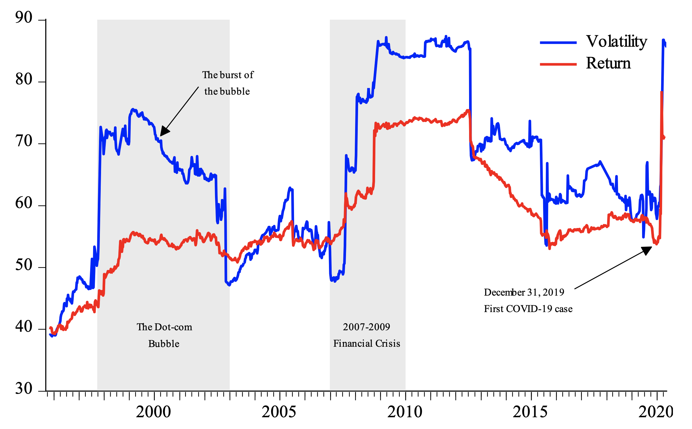
We construct a single graph for both return and volatility spillover over a 200-week rolling window. In Figure 1, two periods are shaded: the dot-com bubble (from its jump in 1997 until 2002, when the NASDAQ lost nearly 80% of its value) and the GFC. We also pinpoint two dates: March 20, 2000, the day the dot-com bubble burst, and December 31, 2019, which when the first case of COVID-19 was reported. In this graph, the presence of a shock in these three periods is quite apparent. At the beginning of each period, we observe a spike in the spillover index, or degree of connectedness. In the case of the dot-com bubble, the shock weakens over time, although, during the GFC, the shock seems to be more persistent. Between these three periods, two more periods of a significant decrease in connectedness are observed. Especially during the 10-year period from 2009 to 2019, the spillover index seems to have a negative trend before it spikes.

IV. Conclusion
In this paper, motivated by recent crises, we examine whether financial markets have remained connected. By extracting a market return and volatility spillover index, we conclude that, in periods of shocks, the connectedness between markets increases. We also show that shock spillover is subsample dependent, that is, they are not constant over time. We demonstrate this through a time-varying spillover shock analysis. The overall message of this paper is that both shocks (the GFC and the COVID-19 pandemic) have had significant impacts on the interdependence between financial markets. We believe that this evidence will be useful in terms of understanding portfolio investment and risk diversification.