Short-Term Prediction of COVID-19 Cases Using Machine Learning Models

Abstract

The first case in Bangladesh of the novel coronavirus disease (COVID-19) was reported on 8 March 2020, with the number of confirmed cases rapidly rising to over 175,000 by July 2020. In the absence of effective treatment, an essential tool of health policy is the modeling and forecasting of the progress of the pandemic. We, therefore, developed a cloud-based machine learning short-term forecasting model for Bangladesh, in which several regression-based machine learning models were applied to infected case data to estimate the number of COVID-19-infected people over the following seven days. This approach can accurately forecast the number of infected cases daily by training the prior 25 days sample data recorded on our web application. The outcomes of these efforts could aid the development and assessment of prevention strategies and identify factors that most affect the spread of COVID-19 infection in Bangladesh.

1. Introduction

The outbreak of the novel coronavirus SARS-CoV2 was first recognized in Wuhan, China [1], and was declared a pandemic by the World Health Organization (WHO) on 11 March 2020 [2]. The Institute of Epidemiology, Disease Control and Research (IEDCR) confirmed the first case in Bangladesh on the 8 March 2020 and the number of infected cases subsequently increased rapidly [3,4,5]. SARS-CoV2 is spread from person to person through physical contact, respiratory droplets, and touching contaminated surfaces [6,7] but the most challenging issue about COVID-19 is that is passed on by infected but asymptomatic individuals. Due to the limited awareness of the disease among the population, complex and uncertain social-political factors increased the wide spread of this virus. Bangladesh is a highly populated country with almost 161.4 million people and a high population density with over 1115 people per square kilometer, and large numbers living in crowded cities and villages [8,9]. Until vaccine access or effective medical treatment, COVID-19 cases will continue to cause a very high death toll. To tackle uncontrolled transmission, the Government of Bangladesh enacted national lockdowns that severely curtailed personal interaction and economic activity [10,11]. For any low or middle income country, most of the population do not have sufficient financial support or savings to survive such a pandemic without working to pay for rent, food, and other necessities. In such a situation, where case numbers are unclear and infection risk is high, it can be difficult to estimate how many people will become infected in particular localities over the the short term. To combat this situation, the government has explored new ways to manage stocks of medical equipment and prepare hospitals by increasing and opening new COVID-19 treatment units and testing labs.

Machine Learning can be utilized to extract useful information from extensive datasets and build intelligent prediction models for healthcare, as well as other features of this viral pandemic [12,13,14,15,16,17]. Along with PCR-based and antibody based virus test predictions, COVID-19 cases can be identified by chest X-ray [18,19] and computerized tomography (CT) [20,21] images using machine learning [22,23]. Besides this, cloud computing has also provided on-demand availability of computing resources such as power and storage [24]. Several resources have thus been developed to forecast ongoing COVID-19 case numbers using a variety of machine learning algorithms. Sujath et al. [25] designed a machine learning forecasting model where linear regression (LR), multilayer perceptron (MLP), and vector autoregression model models were performed on COVID-19 Kaggle data to anticipate case loads in India. Yadav et al. [26] employed machine learning models such as support vector machine (SVM), naïve Bayes (NB), LR, decision tree (DT), random forest (RF), prophet algorithm and long short-term memory (LSTM) to predict COVID-19 cases in different countries. Also, Rustam et al. [6] used different models such as LR, least absolute shrinkage and selection operator (LASSO), SVM and Exponential Smoothing (ES) to predict harmful factors promoting COVID-19 spread. Ardabili et al. [27] compared susceptible, infected and recovered (SIR) as well as susceptible, exposed, infected and recovered (SEIR) models with machine learning and soft computing models, and suggested that machine learning could be an efficient tool to model this outbreak. Zeroual et al. [28] provided a comparative study of five deep learning models such as recurrent neural network (RNN), LSTM, bidirectional LSTM (Bi-LSTM), gated recurrent unit (GRU) and variational autoencoder (VAE) algorithms to forecast infectious cases of Spain, France, China, USA and Australia. Gupta et al. [29] implemented SEIR and regression models to predict COVID-19 cases in India. Wieczorek et al. [30] proposed a neural network model using NAdam where it shows high accuracy to predict COVID-19 cases. Amar et al. [31] applied seven regression models into infectious cases which are exponential, polynomial, quadratic, third degree, fourth degree, fifth degree, sixth degree and logit growth model, respectively. Again, Shahid et al. [32] implemented autoregressive integrated moving average (ARIMA), support vector regressor (SVR), LSTM, Bi-LSTM to manipulate COVID-19 instances, respectively. In the current circumstances, most of the standard epidemiological models, such as SIR [33] or SEIR models, can be used to estimate future case numbers and locations. The effect of COVID-19 on various country-specific sectors has also been studied using computational modeling [34]. Often, these models have not given useful results because they do not properly take into account the non-stationary social mixing parameters prevailing in Bangladesh [27]. Epidemiological data is limited, and it is required to estimate parameters and elaborate automatic transmission models that cannot be accurately interpreted. Therefore, short-term forecasting may be of greater utility in guiding us to understand the patterns of infection spread through the community and suggest the best interventions for minimizing the epidemic [35]. Machine learning models can be used as an alternative means to conventional models for generating short term forecasting based on the reported cases. In addition, these models are also needed to inform rapid actions to counter COVID-19 spread. The integration of cloud services with machine learning models provides an opportunity to greatly improve clinical outcomes above what can be achieved by normal infrastructure alone. Thus, this expected morbidity framework that we propose could greatly assist medical staff to better understand the local and temporal aspects of a dynamic epidemic situation, and so act and communicate accordingly. The objective of this work is therefore to construct a web tool resource that can provide useful forecasts of case numbers and COVID-19-related deaths over the short term future (i.e., 7 days ahead) that employs cloud services readily available in Bangladesh. This work has been shared on the public repository using this following link: https://github.com/shahriariit/Short-Term-Forecasting-BD, accessed on 6 April 2021.

The contribution of this paper is summarized as follows:

1

The number of COVID-19 infected people is currently still increasing inBangladesh but there are only incomplete data on the number and location of cases. There are many strategies for reducing the spread that could be implemented by the local authorities but a lack of understanding of the spreading pattern hinders their design and implementation. We therefore designed software based modeling that can be trained to perform short-term forecasting.

2

Many previous studies have considered many epidemiological models where several pandemic parameters depended on the rate of social mixing of people. In the current circumstances in Bangladesh, we cannot determine or measure such parameters precisely. Therefore, various machine learning models can be a useful approach to forecast infectious cases without needing such parameter precision. However, it is important to note that predictions of infection levels are sensitive to non-linear changes of parameters so that long term prediction tends to give poor results. For this reason, we have focused on implementing short-term forecasting models where accuracy is more likely to be achieved.

3

The analysis with different sliding windows (rounds) helps to estimate the prediction capability of individual machine learning models and assist in the exploration of the best models that provide the most accurate predictions. This model will assist governmental authorities to take more effective steps against COVID-19 spread and fatalities.

4

Cloud based web mining makes it possible to achieve fast and feasible to get real-time outcomes.

This paper is organized as follows—Section 2 provides a brief description of the datasets employed in this paper. This section also explains and discusses the features of the machine learning models and describes the procedures used in the current study. Section 3 then details our experimental results obtained in this analysis, and Section 4 discusses and evaluates the work. Finally, Section 5 summarizes the findings and indicates future directions that may improve this type of analysis.

2. Materials and Methods

2.1. Data Description

Daily COVID-19 prevalence data were retrieved from the GitHub repository of the Center for Systems Science and Engineering (CSSE) at Johns Hopkins University [36] in this structure. The datasets contained regular case reports and time series summary tables. These summaries have been formatted with three tables, such as confirmed infection, fatality and recovered cases of COVID-2019, and contained six attributes, that is, province/state, country/region, last update, confirmed infection, death and recovered cases, where the frequency is updated once a day. Therefore, the cumulative infectious and fatality records have been taken for COVID-19 cases from 8 March to 28 November 2020 as representative case analyses for various stages. We extracted confirmed infection and fatality instances specifying country/region as Bangladesh with our forecasting starting from 14 April 2020.

2.2. Regression Methods

In this framework, we implemented several machine learning regression models to investigate cumulative confirmed infectious and fatality cases in the data constrained environment. To estimate the number of infectious cases, many machine learning models, for example, Linear Regression (LR), Polynomial Regression (PR), Support Vector Regression (SVR), Multi-Layer Perceptron (MLP), Polynomial Multi-Layer perceptron (Poly-MLP), and Prophet algorithm have been applied. However, they were applied to both classification and regression. These models were already used to forecast numerous epidemic diseases such as SARS, Ebola, Cholera, Dengue fever, Swine fever, and H1N1 influenza [27,37]. Recently, some COVID-19 forecasting studies have also performed analyses with these regression models in an effort to model epidemic conditions [6,25,27,30,31,32,38,39]. These studies described good performance of these methods for various types of problem solving and data science competitions. Consequently, we considered these machine learning regression models, which not only performed well for different virus related diseases, but also for COVID-19. In addition, they provided good predictions with a low error rate compared to other models (see Section 3). A brief discussion of these algorithms is given at Appendix A.

Hyperparameter Tuning

Sometimes, different regression models did not show the best results when using their default settings. Therefore, we tuned various parameters of them to improve results. In this case, a parameter named the number of degrees was tuned by PR, SVM and Poly-MLP to get better outcomes. Again, MLP and Poly-MLP were changed the number of neurons to determine the best result. In LR and prophet, there are not found any significant parameters which can improve the findings, hence these classifiers were run in their default settings.

Table 1. The Hyper Parameters of Best Performing Regression Models in Each Round.

Round	Method	Hyperparameters	Method	Hyperparameters
1st Round	Prophet	default	Prophet	default
2nd Round	SVR	degree = 5	SVR	degree = 5
3rd Round	PR	degree = 4	Poly-MLP	degree = 2, neuron = 100
4th Round	PR	degree = 3	Poly-MLP	degree = 1, neuron = 25,13,5
5th Round	Prophet	default	Prophet	default
6th Round	Prophet	default	Prophet	default
7th Round	Prophet	default	Prophet	default
8th Round	Prophet	default	Prophet	default
9th Round	Prophet	default	Prophet	default
10th Round	Prophet	default	Prophet	default
31st Round	Prophet	default	Prophet	default
32nd Round	Prophet	default	Prophet	default
33rd Round	Prophet	default	Prophet	default
34th Round	Prophet	default	Prophet	default
35th Round	Prophet	default	Prophet	default

shows the hyperparameter tuning of different models at each round in this work.

2.3. Cloud Based Services

In this work, we implemented different cloud services to manipulate individual tasks of this web tool. Firstly, the colab notebooks run on Google cloud server that can leverage the power of Google hardware including GPUs and TPUs regardless of the local machine power. These forecasting graphs were then deployed using the plotly Chart Studio cloud service and host it into our local cloud server in the web portal.

2.4. Evaluation Metrics

In regression analysis, the root mean square error (RMSE) is the most widely used evaluation metric for assessing individual regression models. Other metrics, such as Mean Absolute Error (MAE) and R2-Squared, are employed along with RMSE. In this work, a brief description and computation criteria for these are given as below.

2.4.1. Root Mean Square Error (RMSE)

Root mean square error (RMSE) is a quadratic scoring rule that manipulates the average magnitude of inaccuracy. It processes how actual data points focus with the best fit line and is useful for avoiding unexpected large errors. The associated formula regarding this error rate for n instances is given as follow:

$$RMSE=\sqrt{\frac{1}{n}\sum _{i=1}^n{\left(y_i-{\widehat{y}}_i\right)}^2},$$

(1)

where $y_i$ and ${\widehat{y}}_i$ specifies the data points and predicted data points respectively.

2.4.2. Mean Absolute Error (MAE)

Mean absolute error (MAE) determines the average magnitude of the error without considering its direction. It is a linear scoring procedure where all singular differences are weighted in the same way. The matrix values of MAE is also initiated from 0 to infinity and fewer scores represent the good performance of learning models.

$$MAE=\frac{1}{n}\sum _{i=1}^n\left|y_i-{\widehat{y}}_i\right|,$$

(2)

where n, $y_i$ and ${\widehat{y}}_i$ specifies the number of data points, data points and predicted data points, respectively.

2.4.3. R-Squared

R-Squared is a statistical parameter used to assess the performance of regression models. It indicates the strength of the relationship between dependent variables and models, usually described as percentages. This value defines the degree of spread of data points around the prediction lines with 100 percent indicating a data perfectly fits the line. A high $R^2$ value also indicates the goodness-of-fit for the model.

$$R^2=1-\frac{S{S}_{RES}}{S{S}_{TOT}}=1-\frac{{\sum }_i{\left(y_i-{\widehat{y}}_i\right)}^2}{{\sum }_i{\left(y_i-\overline{y}\right)}^2}.$$

(3)

$S{S}_{RES}$ and $S{S}_{TOT}$ indicate the sum of regression and total regression error. $y_i$, ${\widehat{y}}_i$ and $\overline{y}$ denotes as data points, predicted data points and mean values respectively.

2.5. Cloud Based Short Term Forecasting Model: Epidemic Analysis

In this work, we developed a short-term forecasting model that predicts the severity of COVID-19 using various cloud services. The real-time results of this tool are evaluated and broadcasted by our developed web application named COVID-19: Updates, Forecasts and Assistant (https://corona.nstu.edu.bd/, accessed on 21 January 2021). However, it is not a static analysis where the training and forecasting cases of this tool have been updated every 24 h. The working pipeline of the short-term forecasting model is given as follows (see Figure 1):

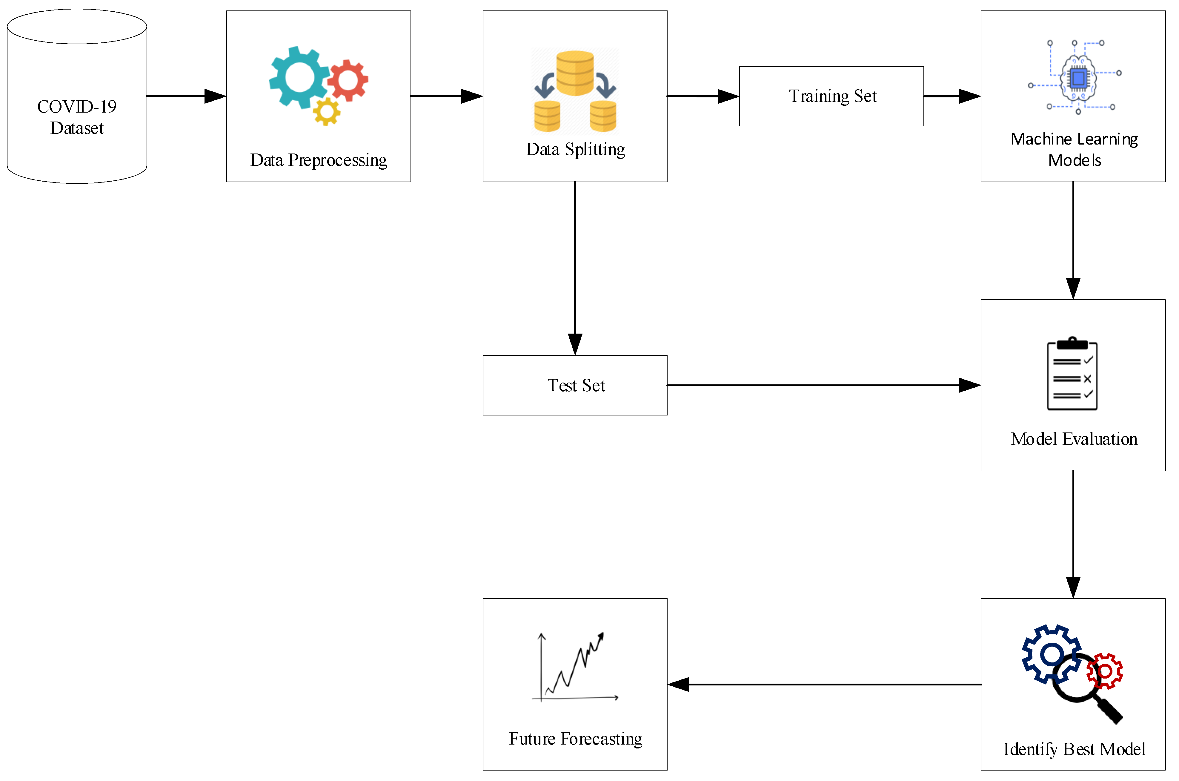
• Firstly, this web tool gathers the daily cumulative instances of confirmed infection and fatality cases of Bangladesh at the Github repository of the Center for Systems Science and Engineering (CSSE) at Johns Hopkins University (see Section 2.1).
• In this work, we gathered the daily cumulative instances from 8 March 2020 to 28 November 2020 where the confirmed infection and fatality cases were investigated to assess the severity of the pandemic in Bangladesh. This whole period was split into several windows using sliding window techniques [40,41]. The size of sliding window was fixed (32 days) and each of them is called round. Instances were identified from the last 25 days where 85% of the data were used as the training set and 15% of the data were used for the the test set. Thus, it analyzes the confirmed infection and fatality cases and forecasts them for the next couple of days as a requirement. For instance, we predicted the next 7 days cases from the training period in this work. Besides this, we considered 35 rounds where the first 10 and last 5 rounds were presented for the next 7 days of future forecasting.
• The primary web mining model was executed on the Google Colab platform. Raw data were loaded and applied using different machine learning regression models which are described in Section 2.2. To explore the best results, parameters need to be estimated and the highest outcomes from them need to be found [27]. However, choosing the optimal parameters is a challenging task for any machine learning procedure. In this work, we manually trained models with various parameters and identified the best model from them.
• To evaluate the performance of different regression models, we used several metrics such as MAE, RMSE and $R^2$ values (see details in Section 2.4) for evaluating the test set and identifying the best model for predicting cumulative confirmed infection and fatality cases with the lowest error rate.
• All actual and predicted trajectories have been placed in our web tool which is uploaded by the local cloud host via plotly Chart Studio.

3. Experiment Result

Forecasting COVID-19 using limited data is a challenging task when we do not have enough accurately measured features for consideration. To estimate confirmed infection and fatality cases, we adopted a simple time series forecasting approach by taking 25 days of cumulative instances for training and test data and generated 7 days of short-term forecasts in Bangladesh. Therefore, we used the scikit learn library to build this tool in Google Colab using python [42].

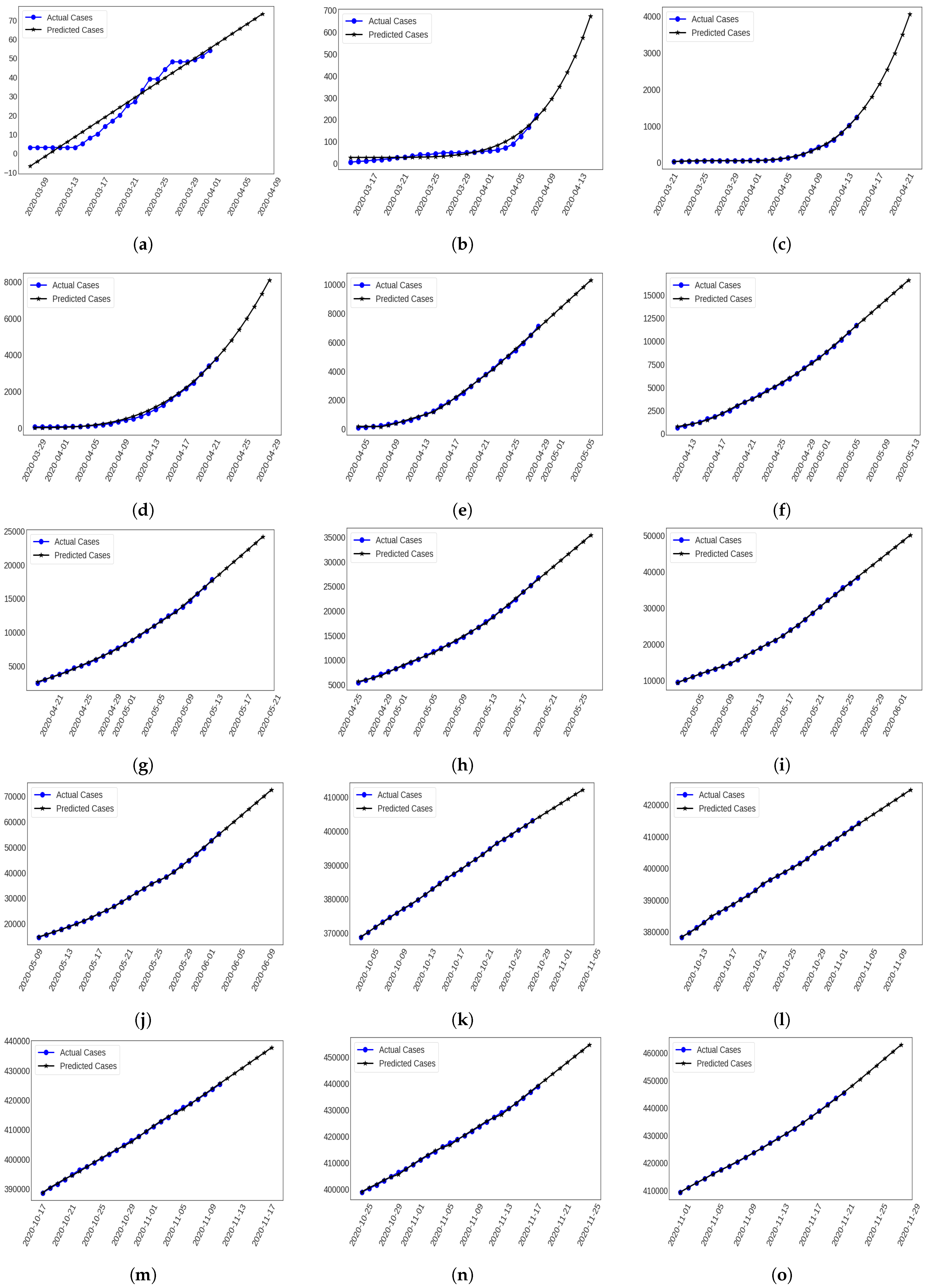
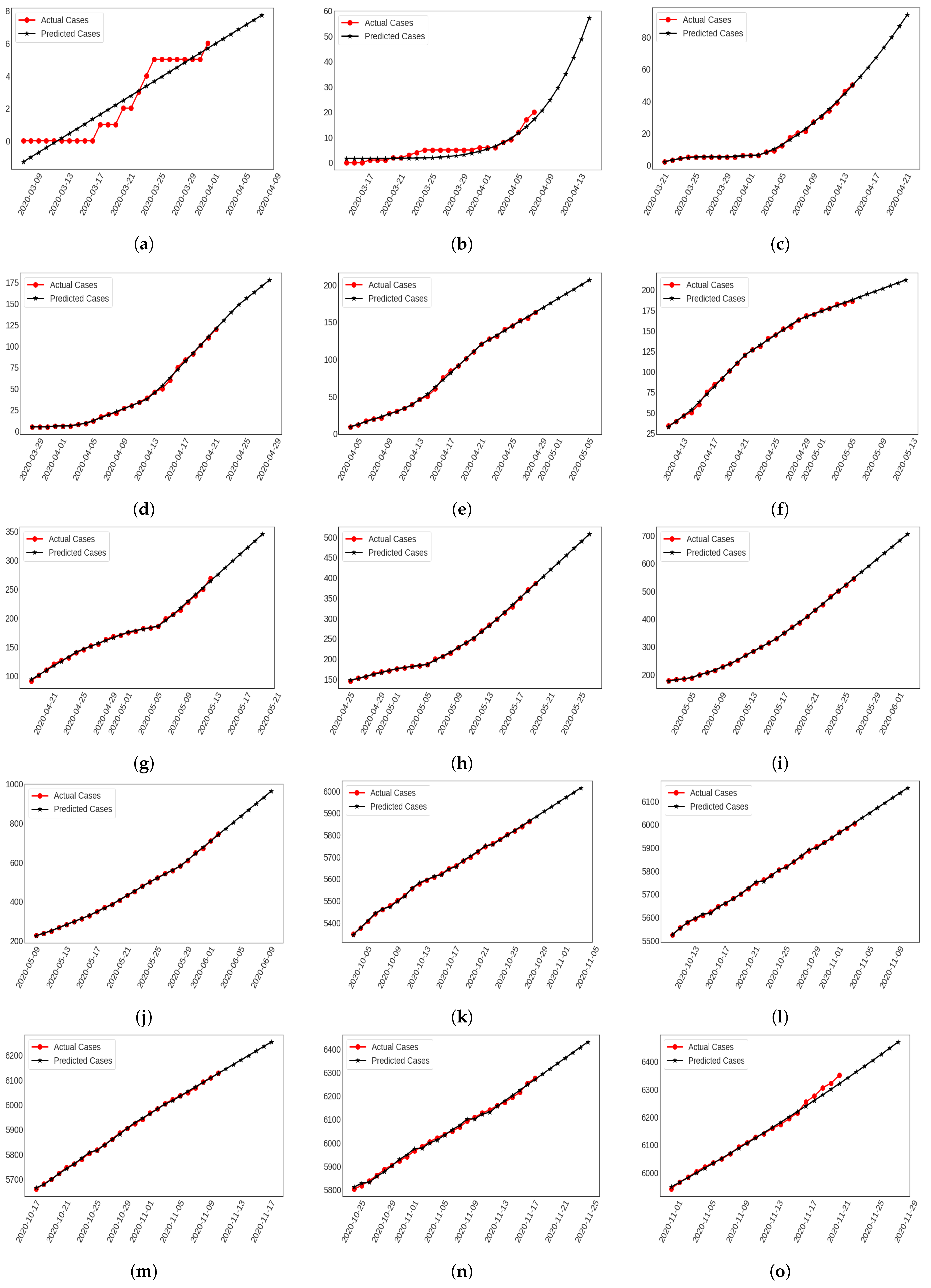
3.1. Cloud Based Short Term Forecasting

We considered a total of 35 rounds to predict confirmed infections and fatalities from the day of detecting the first infectious case in Bangladesh on 12 November 2020. For the sake of simplicity and brevity, we have shown the first 10 rounds of prediction results starting from 8 March 2020 until 10 June 2020, which has been followed by the last 5 rounds of predictions.

3.1.1. 1st Round (8 March 2020–8 April 2020)

In this 1st round, the minimum growth factor was specified as 1 and the maximum factors were found to be 1.667 and 2 for confirmed infection and fatality cases on March 15 and 21, correspondingly (see

Table 2. The Highest Growth Factors of Confirmed Infected Cases and COVID-19-related Fatalites.

Round	Date	Highest Factor		Date	Highest Factor
	Infected Cases			Fatality Cases
1st Round	15-March	1.6670		21-March	2.0000
2nd Round	16-March	1.6000		21-March	2.0000
3rd Round	9-April	1.5138		23-March	1.5000
4th Round	9-April	1.5138		7-April	1.4167
5th Round	9-April	1.5138		7-April	1.4167
6th Round	13-April	1.2930		17-April	1.2500
7th Round	20-April	1.2003		20-April	1.1099
8th Round	29-April	1.0992		13-May	1.0760
9th Round	5-May	1.0775		13-May	1.0760
10th Round	18-May	1.0772		13-May	1.0760
31st Round	07-October	1.0064		14-October	1.0044
32nd Round	12-October	1.0061		14-October	1.0044
33th Round	05-November	1.0044		29-October	1.0054
34th Round	17-November	1.0051		17-November	1.0063
35th Round	19-November	1.0054		17-November	1.0063

). Among 11 regression models, LR showed the lowest RMSE, MAE and highest $R^2$ values for confirmed infection and fatality cases among other models, respectively (see

Table 3. Experimental Results for Both Infected and Fatality Cases from Different Regression Models.

Round	Method	RMSE	MAE	R2		Method	RMSE	MAE	R2
	Infected Cases					Fatality Cases
1st Round	LR	1.0950	1.0489	0.7716		LR	0.2766	0.2500	0.5921
2nd Round	SVR	19.5371	17.4783	0.8372		SVR	2.0445	1.6569	0.7710
3rd Round	PR	13.2350	10.4837	0.9966		Poly-MLP	0.9218	0.8057	0.9777
4th Round	Poly-MLP	53.2986	43.5731	0.9882		MLP	0.7134	0.6773	0.9956
5th Round	Prophet	43.9722	39.9999	0.9951		Prophet	1.0051	0.8383	0.9758
6th Round	Prophet	13.0955	10.9061	0.9998		Prophet	0.5113	0.4621	0.9751
7th Round	Prophet	38.8117	32.6514	0.9989		Prophet	1.7241	1.5615	0.9870
8th Round	Prophet	59.5438	56.5706	0.9987		Prophet	1.8866	1.6031	0.9925
9th Round	Prophet	125.7346	105.7328	0.9946		Prophet	0.8403	0.5109	0.9988
10th Round	Prophet	151.9238	132.1162	0.9974		Prophet	2.8667	2.5618	0.9939
31th Round	Prophet	7.13 $\times {10}^{-11}$	5.82$\times {10}^{-11}$	1.0000		Prophet	9.25$\times {10}^{-12}$	8.41$\times {10}^{-12}$	1.0000
32th Round	Prophet	2.10$\times {10}^{-10}$	1.46$\times {10}^{-10}$	1.0000		Prophet	4.55$\times {10}^{-13}$	2.27$\times {10}^{-13}$	1.0000
33th Round	Prophet	7.70$\times {10}^{-11}$	7.28$\times {10}^{-10}$	1.0000		Prophet	4.55$\times {10}^{-13}$	2.27$\times {10}^{-13}$	1.0000
34th Round	Prophet	2.93$\times {10}^{-09}$	2.49$\times {10}^{-09}$	1.0000		Prophet	1.36$\times {10}^{-12}$	1.14$\times {10}^{-12}$	1.0000
35th Round	Prophet	11.7169	9.0584	0.8144		Prophet	213.5905	201.4884	0.9923

). Although the trend of this model is negative, we ignored the confirmed infection of 8–10 March and fatality cases of 8–12 March 2020. After the training step, we forecasted approximately 58–73 infected cases from 2 to 8 April (see Figure 2a). In the same period, 6–8 fatalities were estimated (see Figure 3a).

3.1.2. 2nd Round (15 March 2020–15 April 2020)

In this round, the regression models were optimized by tuning individual parameters. Moreover, SVR showed the lowest RMSE, MAE and highest $R^2$ values for confirmed infection and fatality cases (see Table 3). In this work, SVR used a polynomial kernel and its number of degrees was 5 for both of these cases. The highest growth factor for death cases (2) was larger than the confirmed infection cases (1.6) in this round (see Table 2). It initiated training with 5 infectious and 0 fatality cases on 15 March up to 5 April 2020. In the 7 days forecasting interval, it estimated 247–672 confirmed infections (see Figure 2b) and 20–57 fatality cases from 9 to 15 April 2020 (see Figure 3b).

3.1.3. 3rd Round (22 March 2020–22 April 2020)

The number of COVID-19 infected individuals were increasing rapidly and PR specified the lowest RMSE, MAE and highest $R^2$ values for confirmed infection cases (the number of degree = 4) and Poly-MLP showed the lowest RMSE, MAE and highest $R^2$ values for fatality cases where the number of degree was 2 and was trained using 100 neurons in this round (see Table 3). In addition, the highest growth factor was 1.5 for confirmed infection and fatality cases correspondingly (see Table 2). In the beginning, this round contained 27 confirmed infectious cases and 2 fatalities on March 22. After the training stage, it predicted almost 1491–4055 confirmed infectious cases (see Figure 2c) and 55–94 fatalities from 16 to 22 April 2020 (see Figure 3c).

3.1.4. 4th Round (29 March 2020–29 April 2020)

In the 4th round, Poly-MLP played the best performance (e.g., number of degrees = 2 and neurons = 100) for confirmed infectious cases and MLP showed the best result (e.g., 25, 13 and 5 neurons) for fatality cases among all other regression models, which are shown in Table 3. In this situation, the growth factor of confirmed infected cases (1.5) increased more than fatality cases (1.4) (see Table 2). Again, it started its training steps on March 29 with 48 confirmed and 5 fatalities. It estimated nearly 4272–8093 confirmed cases (see Figure 2d) and 130–178 death cases (see Figure 3d) from 23 to 29 April 2020.

3.1.5. 5th Round (5 April 2020–6 May 2020)

In the 5th round, it showed 1.5 highest confirmed infection and 1.4 highest death factors (see Table 2). Previously, it started its training process on April 5 with 88 infected and 9 death cases. After implementing different regression models, prophet showed the lowest RMSE, MAE and highest $R^2$ values (see Table 3) and predicted 7431–10,270 confirmed infection cases (see Figure 2e) and 169–203 fatalities (see Figure 3e) from 30 April to 6 May 2020 in this prediction interval.

3.1.6. 6th Round (12 April 2020–13 May 2020)

As indicated in Table 2, the growth factor of infected cases (1.29) was increased by more than the fatality factor (1.25) in the 6th round. The training stages of this analysis were initiated with 621 infected and 34 fatality cases on 12 April 2020. We therefore trained a cumulative sequence of 25 days cases with regression models where prophet showed the lowest RMSE, MAE, and highest $R^2$ values (see Table 3) for the test set. It estimated almost 12,365–16,602 confirmed cases (see Figure 2f) and 191–211 fatality cases (see Figure 3f) from 7 to 13 May 2020.

3.1.7. 7th Round (19 April 2020–20 May 2020)

To forecast cumulative cases more accurately, training was initiated with 2456 confirmed infections and 91 fatality cases on April 29 when the highest growth rate was 1.2 for confirmed infection and 1.1 for fatality cases (see Table 2). Among all regression models, prophet showed the best results which are presented in Table 3. To forecast the next 7 days’ cases, it estimated approximately 18,579–24,182 confirmed infections (see Figure 2g) and 276–345 fatality cases (see Figure 3g) from 14 to 20 May 2020.

3.1.8. 8th Round (26 April 2020–7 May 2020)

In the 8th round, the highest growth factors of confirmed infection and fatality cases were generated as 1.10 and 1.08 on 29 April and 13 May, respectively (see Table 2). At the initial stage, it contained 5416 confirmed infected and 145 fatality cases on 26 April and took the required instances sequentially for training. Again, prophet showed the lowest RMSE, MAE and highest $R^2$ values compared to other regression models (see Table 3). Hence, it predicted more accurately 27,683–35,368 confirmed infected (see Figure 2h) and 402–508 fatality cases (see Figure 3h) on 21 to 27 May 2020, respectively.

3.1.9. 9th Round (3 May 2020–3 June 2020)

The 9th round was started with 9455 confirmed infected and 177 fatality cases where its highest growth factor was 1.08 for infection and fatality cases on 5 and 13 May, respectively (see Table 2). After analyzing the cumulative COVID-19 cases with regression models, prophet showed the best performance in this round (see Table 3). Based on this analysis, it estimated 40,149–50,011 confirmed infected (see Figure 2i) and 568–706 fatality cases (see Figure 3i) from 28 May and 3 June 2020.

3.1.10. 10th Round (10 May 2020–10 June 2020)

The 10th round was begun with 14,657 confirmed infected and 228 fatality cases, including its highest growth factor being 1.07 for confirmed infected and 1.08 for fatality cases (see Table 2). Prophet showed the best performance at forecasting cumulative cases in this round (see Table 3). Moreover, it predicted 57,380–72,367 confirmed infections (see Figure 2j) and 773–964 fatality cases (see Figure 3j) from 4 to 10 June 2020.

3.1.11. 31st Round (4 October 2020–4 November 2020)

In the 31st round the highest growth factors of confirmed infection and fatality cases were provided as 1.006 and 1.004 on 7 and 14 October 2020 (see Table 2) like previous round. The training stages of this analysis started with 368,690 infected and 5348 fatality cases on 4 October 2020. We therefore analyzed a cumulative sequence of 25 days of cases using regression models; prophet showed the lowest RMSE, MAE and highest $R^2$ values (see Table 3) for the test set in this work. It forecasted almost 404,236–412,112 confirmed cases (see Figure 2k) and 5885–6014 fatality cases (see Figure 3k) from 29 October to 4 November 2020.

3.1.12. 32nd Round (11 October 2020–11 November 2020)

Finally, the 32nd round was initiated to train instances with 378,266 confirmed infected and 5524 fatality cases along with its highest growth factor being 1.006 for confirmed infection and 1.004 for fatality cases (see Table 2). Again, prophet showed the best performance to predict cumulated cases in this round (see Table 3). Moreover, it estimated 415,485–424,678 confirmed infections (see Figure 2l) and 6028–6157 fatality cases (see Figure 3l) from 5 to 11 November 2020.

3.1.13. 33rd Round (18 October 2020–18 November 2020)

In the 33rd round, there were initiated 388,569 confirmed infected and 5660 fatality cases where its highest growth factor was 1.004 for confirmed infected and 1.004 for fatality cases (see Table 2). Likewise, prophet provided the maximum results to predict cumulated cases (see Table 3). Moreover, 429,072–437,725 confirmed infections (see Figure 2m) and 6144–6252 fatality cases (see Figure 3m) were estimated from 12 to 18 November 2020.

3.1.14. 34th Round (25 October 2020–25 November 2020)

The 34th round was initiated with 398,815 confirmed infected and 5803 fatality cases along with the highest growth factor was 1.005 for confirmed infected and 1.006 for fatality cases (see Table 2). After investigating them, prophet provided the highest outcomes to predict cumulated cases (see Table 3). Moreover, 441,374–454,618 confirmed infections (see Figure 2n) and 6293–6430 fatality cases (see Figure 3n) were estimated from 19 to 25 November 2020.

3.1.15. 35th Round (1 November 2020–28 November 2020)

In Table 2, the growth factor for infected cases (1.005) was increased more than the fatality factor (1.006) in the 35th round. Initially, it represented 409,252 confirmed infected and 5941 fatality cases on 1 November, then training instances were gathered sequentially. Consequently, PR showed the lowest RMSE, MAE and highest $R^2$ values compared to other regression models (see Table 3). Hence, it predicted 447,928–462,881 confirmed infected (see Figure 2o) and 6408–6715 fatality cases more precisely (see Figure 3o) on 22 to 28 November 2020 respectively.

4. Discussion

In this work, we constructed a short-term forecasting model that trains in a cloud server using data on the cumulative number of reported cases for the COVID-19 pandemic in Bangladesh. It forecasted the infection and fatality cases for the following couple of days quickly and accurately. There have previously been some attempts at this type of statistical modeling [43] around COVID-19 in Bangladesh that have shown some success. However, our proposed improved model employs a comprehensive machine learning prediction model to investigate cumulative cases which yielded a very good fit to the epidemic curves when it conducts its evaluations using RMSE, MAE and $R^2$ values.

It is notable that individual rounds provide trends of the epidemic curve, which are observed in this analysis. In the 1st round, LR showed the best result because the cumulative cases were not much increased during this period. However, the trend or growth factor increased markedly from the 1st to the 4th round, showed the best performance for SVM, PR, MLP, or Poly-MLP using hyperparameter tuning. Through the rest of the rounds (for the 5th, 6th, 7th, 8th, 9th and 10th), we investigated the results of machine learning regression models, and found that the prophet model gave the best results for both infections and mortalities. From the 5th to the 9th rounds, it indicated the increased rate of growth factor for confirmed infection than death cases. However, their differences are not large. Nevertheless, the growth rate of fatalities is increased compared to the confirmed infection rate in the 10th round. However, the growth factor did not vary more, hence prophet showed the best results consistently from the 5th to the 10th round. Besides,

Table 4. Execution Time of Individual Rounds.

Round	LR	PR	SVR	MLP	Poly-MLP	Prophet
1st Round	0.467	0.603	0.666	1.673	1.314	0.450
2nd Round	0.468	0.431	0.483	1.201	1.201	0.433
3rd Round	0.452	0.444	0.451	3.557	2.609	4.012
4th Round	0.459	0.454	0.457	6.173	7.149	4.189
5th Round	0.471	0.432	0.465	6.842	8.127	4.613
6th Round	0.724	0.457	0.466	11.836	9.134	4.560
7th Round	0.522	0.456	0.437	13.691	10.809	4.501
8th Round	0.466	0.703	0.470	12.593	12.404	4.693
9th Round	0.445	0.460	0.476	8.051	10.579	4.520
10th Round	0.471	0.458	0.452	8.013	8.801	4.737
31st Round	0.515	0.656	0.665	8.532	7.510	35.499
32nd Round	0.471	0.483	0.459	8.657	8.002	30.286
33rd Round	0.493	0.723	0.512	8.764	7.590	23.994
34th Round	0.485	0.475	0.751	8.727	7.762	28.945
35th Round	0.500	0.463	0.477	9.043	7.848	0.459

shows the average execution times of different methods where prophet algorithms takes more time than others. The runtime of the prophet algorithm is also higher from the 31st to the 34th round, respectively. Nevertheless, this algorithm generated a low error rate in forecasting associated cases, hence it has been taken as the best model in most of the rounds. To justify the consistency of these results, we split primary dataset into 75:25 ratio where 75% instances were trained and 25% records were used as test sets. Similar models were then implemented into these datasets and manipulated the error rates (see

Table 5. Verification of Experimental Results for Infected and Fatality Cases.

Round	Method	RMSE	MAE	R2	Method	RMSE	MAE	R2
		Confirmed Cases				Death Cases
1st Round	Prophet	3.5808	2.7740	−0.5786	Prophet	0.5837	0.4524	−1.7821
2nd Round	SVR	24.8737	22.8440	0.8043	SVR	2.4589	2.2902	0.7660
3rd Round	PR	55.1576	49.7568	0.9676	Poly-MLP	2.3675	2.1407	0.9394
4th Round	PR	63.7025	57.3959	0.9928	Poly-MLP	5.8317	4.9376	0.9072
5th Round	Prophet	36.9007	31.2751	0.9985	Prophet	1.3350	1.0758	0.9877
6th Round	Prophet	10.9600	9.0326	0.9999	Prophet	0.7154	0.6148	0.9870
7th Round	Prophet	38.8742	34.5744	0.9995	Prophet	1.5454	1.4078	0.9956
8th Round	Prophet	51.7929	46.3280	0.9996	Prophet	1.4812	1.1691	0.9982
9th Round	Prophet	117.2432	98.1062	0.9987	Prophet	0.8894	0.6813	0.9996
10th Round	Prophet	155.8378	131.5769	0.9990	Prophet	2.2835	1.8957	0.9987
31st Round	Prophet	6.22$\times {10}^{-11}$	4.99$\times {10}^{-11}$	1.0000	Prophet	9.27$\times {10}^{-12}$	8.71$\times {10}^{-12}$	1.0000
32nd Round	Prophet	1.89$\times {10}^{-10}$	1.50$\times {10}^{-10}$	1.0000	Prophet	4.86$\times {10}^{-13}$	2.60$\times {10}^{-13}$	1.0000
33rd Round	Prophet	7.93$\times {10}^{-11}$	7.48$\times {10}^{-11}$	1.0000	Prophet	4.86$\times {10}^{-13}$	2.60$\times {10}^{-13}$	1.0000
34th Round	Prophet	3.11$\times {10}^{-09}$	2.63$\times {10}^{-09}$	1.0000	Prophet	1.33$\times {10}^{-12}$	1.17$\times {10}^{-12}$	1.0000
35th Round	Prophet	4.40$\times {10}^{-11}$	3.33$\times {10}^{-11}$	1.0000	Prophet	8.21$\times {10}^{-11}$	7.04$\times {10}^{-11}$	1.0000

). Without the 1st and 4th rounds, all regression models showed consistent results as well. Numerous research groups have attempted to forecast infectious cases, such as [6,44,45], but did not verify their models using several intervals or rounds. Some of these [25] did not evaluate their work using appropriate evaluation metrics. Our model is implemented on a cloud based web portal (https://corona.nstu.edu.bd/, accessed on 21 January 2021) and dynamically predicted confirmed both infection and fatality cases with high consistency [46].

In previous studies of diseases, epidemiological models require a number of parameters related to social mixing to fit models well. However, contact tracing has found this is non-stationary through time due to unreliable social interaction parameters. In SIR or SEIR, social mixing alters the number of susceptible individuals and the reproductive number $R_0$. If $R_0$ is greater than 1, then it will spread. When it is less than 1, then the epidemic may decrease and eventually disappear. In addition, it is clear that such models must be adapted to the local situation based on insights into susceptibility to confirmed infection. For Bangladesh, conventional epidemiological models face substantial limits to obtaining a generalized prediction ability and robustness. Therefore, machine learning has gained a great deal of attention, resulting in numerous attempts to develop a disease outbreak prediction tool that shows high generalization and reliability. These models can empower individuals and organisations to estimate infection and fatality cases in the near future and take rapid decisions about public health measures that counter it.

Implications

This application likely has a useful impact on people, organizations and society. In the pandemic situation, people are suffering from financial crisis and cannot engage in their work due to lockdowns that mean they cannot go outside of their home. This has severe economic effects on individuals and also affects their psychological condition. Various organizations have reduced their activities due to this persistent pandemic which in turn hampered their business and led to large financial losses. In such scenarios, knowing the pandemic condition and the probable number of cases in the near future becomes important. The proposed short-term forecasting model is more useful for giving a perfect prediction about how many people will be infected or die. It gives real-time forecasting by training recent instances. Therefore, individuals can be updated about the pandemic situation and can make appropriate plans on how to plan their work and activities. Hence, organizations are interested in minimizing their losses by receiving COVID-19 updates from models such as this.

5. Conclusions and Future Work

Importantly, confirmed infections and fatality cases were defined, and influenced the testing capacity of Bangladesh. Again, it indicated other related factors such as lockdown, curfew, quarantine, and suspect infected zones according to the reporting date. During this pandemic period, the prediction shows the number of confirmed infections and fatality cases were rising rapidly in Bangladesh. Furthermore, there were notable delays in identifying and isolating cases due to the magnitude of the pandemic. Our cloud-based short-term forecasting model can aid real-time decision making that will be needed to prepare, such as anticipating the amount of equipment, beds for treatment in the hospital, and other medical resources that will be needed. In addition, the cloud server manipulates time-series instances and forecasts that are easy and rapid. We evaluated time-series COVID-19 dataset using different regression models and the prophet algorithm shows the lowest error rate in most of the rounds. Thus, prophet can be estimated as a more stable regression model than others. However, there are some limitations; for instance, it does not provide functions such as region or person-to-person contact tracing, which is more useful for identifying affected cases in Bangladesh. In the future, these issues will be addressed and a more appropriate model to forecast cumulative instances will be prepared. We will utilize more machine learning techniques to estimate missing information about exposed and infected persons and fit it to conventional epidemiological models.

References

1. Sarkodie, S.A.; Owusu, P.A. Investigating the cases of novel coronavirus disease (COVID-19) in China using dynamic statistical techniques. Heliyon 2020, 6, e03747. [Google Scholar] [CrossRef]
2. Shawni, D.; Bandyopadhyay, S.K. Machine learning approach for confirmation of COVID-19 cases: Positive, negative, death and release. Iberoam. J. Med. 2020, 2, 172–177. [Google Scholar] [CrossRef]
3. Islam, M.T.; Talukder, A.K.; Siddiqui, M.N.; Islam, T. Tackling the COVID-19 pandemic: The Bangladesh perspective. J. Public Health Res. 2020, 9. [Google Scholar] [CrossRef] [PubMed]
4. Ahamad, M.; Aktar, S.; Rashed-Al-Mahfuz, M.; Azad, A.; Uddin, S.; Alyami, S.A.; Sarker, I.H.; Liò, P.; Quinn, J.M.W.; Moni, M.A. Adverse effects of COVID-19 vaccination: Machine learning and statistical approach to identify and classify incidences of morbidity and post-vaccination reactogenicity. medrXiv 2021. [Google Scholar] [CrossRef]
5. Uddin, S.; Imam, T.; Ali Moni, M. The implementation of public health and economic measures during the first wave of COVID-19 by different countries with respect to time, infection rate and death rate. In 2021 Australasian Computer Science Week Multiconference; Association for Computing Machinery: New York, NY, USA, 2021; pp. 1–8. [Google Scholar] [CrossRef]
6. Rustam, F.; Reshi, A.A.; Mehmood, A.; Ullah, S.; On, B.; Aslam, W.; Choi, G.S. COVID-19 Future Forecasting Using Supervised Machine Learning Models. IEEE Access 2020, 8, 101489–101499. [Google Scholar] [CrossRef]
7. Ahamad, M.M.; Aktar, S.; Rashed-Al-Mahfuz, M.; Uddin, S.; Liò, P.; Xu, H.; Summers, M.A.; Quinn, J.M.; Moni, M.A. A machine learning model to identify early stage symptoms of SARS-Cov-2 infected patients. Expert Syst. Appl. 2020, 160, 113661. [Google Scholar] [CrossRef]
8. Satu, M.; Howlader, K.C.; Islam, S.M.S. Machine Learning-Based Approaches for Forecasting COVID-19 Cases in Bangladesh; SSRN Scholarly Paper ID 3614675; Social Science Research Network: Rochester, NY, USA, 2020. [Google Scholar] [CrossRef]
9. Aktar, S.; Ahamad, M.; Rashed-Al-Mahfuz, M.; Azad, A.; Uddin, S.; Kamal, A.; Alyami, S.A.; Lin, P.I.; Islam, S.M.S.; Quinn, J.M.; et al. Predicting Patient COVID-19 Disease Severity by means of Statistical and Machine Learning Analysis of Blood Cell Transcriptome Data. arXiv 2020, arXiv:2011.10657. [Google Scholar]
10. Kolhar, M.; Al-Turjman, F.; Alameen, A.; Abualhaj, M.M. A three layered decentralized IoT biometric architecture for city lockdown during COVID-19 outbreak. IEEE Access 2020, 8, 163608–163617. [Google Scholar] [CrossRef]
11. Rahman, M.A.; Zaman, N.; Asyhari, A.T.; Al-Turjman, F.; Alam Bhuiyan, M.Z.; Zolkipli, M.F. Data-driven dynamic clustering framework for mitigating the adverse economic impact of Covid-19 lockdown practices. Sustain. Cities Soc. 2020, 62, 102372. [Google Scholar] [CrossRef]
12. Kalajdjieski, J.; Zdravevski, E.; Corizzo, R.; Lameski, P.; Kalajdziski, S.; Pires, I.M.; Garcia, N.M.; Trajkovik, V. Air Pollution Prediction with Multi-Modal Data and Deep Neural Networks. Remote Sens. 2020, 12, 4142. [Google Scholar] [CrossRef]
13. Liu, P.; Wang, J.; Sangaiah, A.K.; Xie, Y.; Yin, X. Analysis and Prediction of Water Quality Using LSTM Deep Neural Networks in IoT Environment. Sustainability 2019, 11, 2058. [Google Scholar] [CrossRef] [Green Version]
14. Ceci, M.; Corizzo, R.; Japkowicz, N.; Mignone, P.; Pio, G. ECHAD: Embedding-Based Change Detection From Multivariate Time Series in Smart Grids. IEEE Access 2020, 8, 156053–156066. [Google Scholar] [CrossRef]
15. Aktar, S.; Ahamad, M.M.; Rashed-Al-Mahfuz, M.; Azad, A.; Uddin, S.; Kamal, A.; Alyami, S.A.; Lin, P.I.; Islam, S.M.S.; Quinn, J.M.; et al. Machine Learning Approach to Predicting COVID-19 Disease Severity Based on Clinical Blood Test Data: Statistical Analysis and Model Development. JMIR Med. Inf. 2021, 9, e25884. [Google Scholar] [CrossRef] [PubMed]
16. Corizzo, R.; Ceci, M.; Fanaee-T, H.; Gama, J. Multi-aspect renewable energy forecasting. Inf. Sci. 2021, 546, 701–722. [Google Scholar] [CrossRef]
17. Satu, M.S.; Khan, M.I.; Mahmud, M.; Uddin, S.; Summers, M.A.; Quinn, J.M.; Moni, M.A. TClustVID: A Novel Machine Learning Classification Model to Investigate Topics and Sentiment in COVID-19 Tweets. MedRxiv 2020. [Google Scholar] [CrossRef]
18. Satu, M.S.; Ahammed, K.; Abedin, M.Z.; Rahman, M.A.; Islam, S.M.S.; Azad, A.; Alyami, S.A.; Moni, M.A. Convolutional Neural Network Model to Detect COVID-19 Patients Utilizing Chest X-ray Images. medRxiv 2021. [Google Scholar] [CrossRef]
19. Aradhya, V.N.M.; Mahmud, M.; Guru, D.; Agarwal, B.; Kaiser, M.S. One-shot Cluster-Based Approach for the Detection of COVID–19 from Chest X–ray Images. Cogn. Comput. 2021, 1–8. [Google Scholar] [CrossRef]
20. Depeursinge, A.; Chin, A.S.; Leung, A.N.; Terrone, D.; Bristow, M.; Rosen, G.; Rubin, D.L. Automated classification of usual interstitial pneumonia using regional volumetric texture analysis in high-resolution CT. Investig. Radiol. 2015, 50, 261. [Google Scholar] [CrossRef]
21. Dey, N.; Rajinikanth, V.; Fong, S.J.; Kaiser, M.S.; Mahmud, M. Social Group Optimization–Assisted Kapur’s Entropy and Morphological Segmentation for Automated Detection of COVID-19 Infection from Computed Tomography Images. Cogn. Comput. 2020, 12, 1011–1023. [Google Scholar] [CrossRef]
22. Waheed, A.; Goyal, M.; Gupta, D.; Khanna, A.; Al-Turjman, F.; Pinheiro, P.R. CovidGAN: Data Augmentation Using Auxiliary Classifier GAN for Improved Covid-19 Detection. IEEE Access 2020, 8, 91916–91923. [Google Scholar] [CrossRef]
23. Aktar, S.; Talukder, A.; Ahamad, M.; Kamal, A.; Khan, J.R.; Protikuzzaman, M.; Hossain, N.; Quinn, J.M.; Summers, M.A.; Liaw, T.; et al. Machine Learning and Meta-Analysis Approach to Identify Patient Comorbidities and Symptoms that Increased Risk of Mortality in COVID-19. arXiv 2020, arXiv:2008.12683. [Google Scholar]
24. Al-Turjman, F.; Deebak, B. Privacy-Aware Energy-Efficient Framework Using the Internet of Medical Things for COVID-19. IEEE Internet Things Mag. 2020, 3, 64–68. [Google Scholar] [CrossRef]
25. Sujath, R.; Chatterjee, J.M.; Hassanien, A.E. A machine learning forecasting model for COVID-19 pandemic in India. Stoch. Environ. Res. Risk Assess. 2020, 34, 959–972. [Google Scholar] [CrossRef]
26. Yadav, D.; Maheshwari, H.; Chandra, U.; Sharma, A. COVID-19 Analysis by Using Machine and Deep Learning. In Internet of Medical Things for Smart Healthcare: Covid-19 Pandemic; Chakraborty, C., Banerjee, A., Garg, L., Rodrigues, J.J.P.C., Eds.; Studies in Big Data; Springer: Singapore, 2020; pp. 31–63. [Google Scholar] [CrossRef]
27. Ardabili, S.F.; Mosavi, A.; Ghamisi, P.; Ferdinand, F.; Varkonyi-Koczy, A.R.; Reuter, U.; Rabczuk, T.; Atkinson, P.M. COVID-19 Outbreak Prediction with Machine Learning. Algorithms 2020, 13, 249. [Google Scholar] [CrossRef]
28. Zeroual, A.; Harrou, F.; Dairi, A.; Sun, Y. Deep learning methods for forecasting COVID-19 time-Series data: A Comparative study. Chaos Solitons Fractals 2020, 140, 110121. [Google Scholar] [CrossRef] [PubMed]
29. Gupta, R.; Pandey, G.; Chaudhary, P.; Pal, S.K. Machine Learning Models for Government to Predict COVID-19 Outbreak. Digit. Gov. Res. Pract. 2020, 1, 1–6. [Google Scholar] [CrossRef]
30. Wieczorek, M.; Siłka, J.; Woźniak, M. Neural network powered COVID-19 spread forecasting model. Chaos Solitons Fractals 2020, 140, 110203. [Google Scholar] [CrossRef] [PubMed]
31. Amar, L.A.; Taha, A.A.; Mohamed, M.Y. Prediction of the final size for COVID-19 epidemic using machine learning: A case study of Egypt. Infect. Dis. Model. 2020, 5, 622–634. [Google Scholar] [CrossRef] [PubMed]
32. Shahid, F.; Zameer, A.; Muneeb, M. Predictions for COVID-19 with deep learning models of LSTM, GRU and Bi-LSTM. Chaos Solitons Fractals 2020, 140, 110212. [Google Scholar] [CrossRef]
33. Srivastava, V.; Srivastava, S.; Chaudhary, G.; Al-Turjman, F. A systematic approach for COVID-19 predictions and parameter estimation. Pers. Ubiquitous Comput. 2020. [Google Scholar] [CrossRef]
34. Kumar, S.; Viral, R.; Deep, V.; Sharma, P.; Kumar, M.; Mahmud, M.; Stephan, T. Forecasting major impacts of COVID-19 pandemic on country-driven sectors: Challenges, lessons, and future roadmap. Pers. Ubiquitous Comput. 2021. [Google Scholar] [CrossRef] [PubMed]
35. Roosa, K.; Lee, Y.; Luo, R.; Kirpich, A.; Rothenberg, R.; Hyman, J.; Yan, P.; Chowell, G. Real-time forecasts of the COVID-19 epidemic in China from February 5th to February 24th, 2020. Infect. Dis. Model. 2020, 5, 256–263. [Google Scholar] [CrossRef]
36. Dong, E.; Du, H.; Gardner, L. An interactive web-based dashboard to track COVID-19 in real time. Lancet Infect. Dis. 2020, 20, 533–534. [Google Scholar] [CrossRef]
37. Pandey, M.K.; Subbiah, K. Performance Analysis of Time Series Forecasting Using Machine Learning Algorithms for Prediction of Ebola Casualties. In International Conference on Application of Computing and Communication Technologies; Communications in Computer and Information Science; Deka, G.C., Kaiwartya, O., Vashisth, P., Rathee, P., Eds.; Springer: Singapore, 2018; pp. 320–334. [Google Scholar]
38. Ribeiro, M.H.D.M.; da Silva, R.G.; Mariani, V.C.; dos Santos Coelho, L. Short-term forecasting COVID-19 cumulative confirmed cases: Perspectives for Brazil. Chaos Solitons Fractals 2020, 135, 109853. [Google Scholar] [CrossRef] [PubMed]
39. Wang, P.; Zheng, X.; Li, J.; Zhu, B. Prediction of epidemic trends in COVID-19 with logistic model and machine learning techniques. Chaos Solitons Fractals 2020, 139, 110058. [Google Scholar] [CrossRef]
40. Alberg, D.; Last, M. Short-term load forecasting in smart meters with sliding window-based ARIMA algorithms. Vietnam. J. Comput. Sci. 2018, 5, 241–249. [Google Scholar] [CrossRef]
41. Khan, I.A.; Akber, A.; Xu, Y. Sliding window regression based short-term load forecasting of a multi-area power system. In Proceedings of the 2019 IEEE Canadian Conference of Electrical and Computer Engineering (CCECE), Edmonton, AB, Canada, 5–8 May 2019; pp. 1–5. [Google Scholar]
42. Pedregosa, F.; Varoquaux, G.; Gramfort, A.; Michel, V.; Thirion, B.; Grisel, O.; Blondel, M.; Prettenhofer, P.; Weiss, R.; Dubourg, V.; et al. Scikit-learn: Machine Learning in Python. J. Mach. Learn. Res. 2011, 12, 2825–2830. [Google Scholar]
43. Khan, M.H.R.; Hossain, A. COVID-19 Outbreak Situations in Bangladesh: An Empirical Analysis. medRxiv 2020. [Google Scholar] [CrossRef]
44. Punn, N.S.; Sonbhadra, S.K.; Agarwal, S. COVID-19 Epidemic Analysis using Machine Learning and Deep Learning Algorithms. medRxiv 2020. [Google Scholar] [CrossRef] [Green Version]
45. Ndiaye, B.M.; Tendeng, L.; Seck, D. Analysis of the COVID-19 pandemic by SIR model and machine learning technics for forecasting. arXiv 2020, arXiv:2004.01574. [Google Scholar]
46. Satu, M.S.; Rahman, M.K.; Rony, M.A.; Shovon, A.R.; Adnan, M.J.A.; Howlader, K.C.; Kaiser, M.S. COVID-19: Update, Forecast and Assistant-An Interactive Web Portal to Provide Real-Time Information and Forecast COVID-19 Cases in Bangladesh. In Proceedings of the 2021 International Conference on Information and Communication Technology for Sustainable Development (ICICT4SD), Dhaka, Bangladesh, 27–28 February 2021; pp. 456–460. [Google Scholar]
47. Han, J.; Pei, J.; Kamber, M. Data Mining: Concepts and Techniques; Elsevier: Amsterdam, The Netherlands, 2011. [Google Scholar]
48. Akter, T.; Satu, M.S.; Khan, M.I.; Ali, M.H.; Uddin, S.; Lio, P.; Quinn, J.M.; Moni, M.A. Machine learning-based models for early stage detection of autism spectrum disorders. IEEE Access 2019, 7, 166509–166527. [Google Scholar] [CrossRef]
49. Uddin, S.; Khan, A.; Hossain, M.E.; Moni, M.A. Comparing different supervised machine learning algorithms for disease prediction. BMC Med. Inf. Decis. Mak. 2019, 19, 1–16. [Google Scholar] [CrossRef]
50. Moula, F.E.; Guotai, C.; Abedin, M.Z. Credit default prediction modeling: An application of support vector machine. Risk Manag. 2017, 19, 158–187. [Google Scholar] [CrossRef]
51. Hu, Y.C. Multilayer perceptron for robust nonlinear interval regression analysis using genetic algorithms. Sci. World J. 2014, 2014, 970931. [Google Scholar] [CrossRef] [PubMed]
52. Taylor, S.J.; Letham, B. Forecasting at scale. Am. Stat. 2018, 72, 37–45. [Google Scholar] [CrossRef]
Figure 1. Cloud based Short-Term Forecasting Model.
Applsci 11 04266 g001
Figure 2. Future Forecasting of Confirmed Cases estimating (a) 1st round by LR (b) 2nd round by SVM (c) 3rd round by PR (d) 4th round by Poly-MLP including (e) 5th (f) 6th (g) 7th (h) 8th (i) 9th (j) 10th (k) 31th (l) 32th (m) 33th (n) 34th round by Prophet Algorithm and (o) 35th round by PR.
Applsci 11 04266 g002
Figure 3. Future Forecasting of Death Cases estimating (a) 1st round by LR (b) 2nd round by SVM (c) 3rd round by Poly-MLP (d) 4th round by MLP including (e) 5th (f) 6th (g) 7th (h) 8th (i) 9th (j) 10th (k) 31th (l) 32th (m) 33th (n) 34th round by Prophet Algorithm and (o) 35th round by PR.
Applsci 11 04266 g003