Forecasting a New Type of Virus Spread: A Case Study of COVID-19 with Stochastic Parameters

Abstract

The consideration of infectious diseases from a mathematical point of view can reveal possible options for epidemic control and fighting the spread of infection. However, predicting and modeling the spread of a new, previously unexplored virus is still difficult. The present paper examines the possibility of using a new approach to predicting the statistical indicators of the epidemic of a new type of virus based on the example of COVID-19. The important result of the study is the description of the principle of dynamic balance of epidemiological processes, which has not been previously used by other researchers for epidemic modeling. The new approach is also based on solving the problem of predicting the future dynamics of precisely random values of model parameters, which is used for defining the future values of the total number of: cases (C); recovered and dead (R); and active cases (I). Intelligent heuristic algorithms are proposed for calculating the future trajectories of stochastic parameters, which are called the percentage increase in the total number of confirmed cases of the disease and the dynamic characteristics of epidemiological processes. Examples are given of the application of the proposed approach for making forecasts of the considered indicators of the COVID-19 epidemic, in Russia and European countries, during the first wave of the epidemic.

1. Introduction

An outbreak of the coronavirus infection, COVID-19, caused by the new SARS-CoV-2 virus, quickly spread around the world at the end of 2019, affecting more than 200 countries. The consideration of infectious diseases caused by new, previously unexplored viruses from a mathematical point of view can reveal not only the important patterns of a pandemic, but also possible options for epidemic control and fighting the spread of infection. Mathematical models of disease transmission, as most experts note, can help to gain insight into the dynamics of the spread of infectious diseases and the potential role of different types of public health intervention strategies. The main problem in the absence of the availability of historical data for modeling the spread of a new virus arises when estimating the values of the input parameters of a particular model. Given the maximum uncertainty in the parameters of the spread of a new virus, difficulties naturally arise in assessing the potential dangers and scale of the epidemic. Traditionally used parameters in the classic Susceptible—Infected—Recovered (SIR)) model cannot be quantified with sufficient accuracy, which does not allow for eliminating the uncertainty of the future dynamics of coronavirus spread. The aim of this work is to study the possibilities of using a case-based rate reasoning (CBRR) model for predicting the rates of COVID-19 spread in Russia and extending it to other countries. The proposed approach considers the percentage increase as one of the most important parameters of the forecasting model, which has a stochastic nature. As part of the approach being developed, it is proposed to evaluate the trends in the key parameters, such as the percentage increase in the number of confirmed cases of the disease and the percentage increase in the number of deaths, and use the resulting trends in the subsequent forecast of the main statistical epidemic spread indicators’ dynamics. Another important parameter is the so-called dynamic balance characteristic. It is based on the proposed principle of dynamic balance of epidemiological processes, which has not been previously used in models of epidemic spread. The new approach is based, first of all, on solving the problem of predicting the future dynamics of precisely random values of model parameters, instead of the values of real-time data. Predictive trajectories of the future values of epidemic data (the total number of confirmed cases (C), the number of active cases of the disease (I), and the dynamics of the total number of recovered (R) and dead (D)) were calculated by substituting into the model the values of these random parameters obtained during the analytical study. In the future, this algorithm could be used in modeling complex network systems with emergent intelligence.

2. Literature Overview

A systematic review of the models for predicting epidemics of the novel SARS-CoV-2 (COVID-19) coronavirus was conducted by the authors. The search was carried out in the Web of Science, Scopus and RCI databases. Additionally, the search results were analyzed in the Elsevier database, one of the largest European publishers. The following keywords were used: “forecasting”, “prediction”, “model”, “emerging infection”, “coronavirus” and “COVID”. There are also several web portals aggregating research related to coronavirus such as, for example, according to the World Health Organization [1]. During the search, special attention was paid to studies related to forecasting models for the dynamics of the epidemic spread in the first wave, when there was a lack of information about the new coronavirus and the population did not develop immunity to the new infection. In general, there are four main approaches to modeling the spread of infectious diseases [2]: time series-based models, compartment models, agent-based (network) models, and models built using machine learning methods and heuristic approaches.

Regarding time-series based models, it should be noted that regression analysis and time series analysis are among the most well-known methods for predicting the incidence of a disease. Several researchers have used the Autoregressive Integrated Moving Average (ARIMA) model to predict the spread of the novel coronavirus pandemic. Examples of such studies include [3,4,5,6]. In general, although time series models are a popular forecasting tool, the use of this approach to estimate the spread of new infections has its limitations. In particular, the lack of statistics for previous periods and, as a consequence, unknown parameter values, do not allow building models of a sufficient degree of accuracy.

Most of the research is based on the Susceptible—Infected—Recovered (SIR) paradigm and its variations, which is described as a system of ordinary differential equations [7]. In the basic compartment model, a population of N people is considered. At each moment in time, each person belongs to one of the three groups (compartments): the Susceptible group (S), including people who have not yet encountered an infection; then, as the virus spreads among the population, they move to the Infected group (I); and then, into the Removed (R) group (recovered or deceased). The possibility of reinfection in this model is not taken into consideration. It is also assumed that the size of the population remains unchanged. The so-called SIR epidemic model, described as a system of three ordinary differential equations for the variables S, I and R, was presented for the first time in a paper by Kermack and McKendrick in 1927 [8,9].

Many researchers prefer to use the SIR model because of the small number of input parameters required. However, sometimes this advantage arises from the oversimplification of the model due to relatively unrealistic assumptions. For example, the model assumes the homogeneous mixing of the population, which means that all individuals in the population are equally likely to come into contact with each other. This does not reflect the human social structures in which most contact occurs in localized communities. The SIR model also assumes a closed population with no migration, births or deaths from causes other than epidemics. In addition to the SIR model, various modifications of it are often used such as, for example, the SEIR model, which adds an Exposed (E) parameter for people who have already been infected but are not yet infectious, as well as the SIRD model, which provides separate parameters for recovered people (those who survived the disease and are now immune) and deceased people. In general, up to the present, only several dozen SIR models and their varieties have been published on COVID-19. In particular, these have been the SIR [10,11,12,13], SEIR [14,15,16,17,18,19,20,21,22], SIRD [23,24], SIR-X [25], SEIQR [26] and SEIHR [27] models.

Special mention should be made of research devoted to models that take into account the delay of input parameters [28,29,30,31,32,33]. Mostly, these research models are focused on evaluating the parameters of compartment models based on the assumptions about the delay between the diagnosis and the time of infection.

Network models can be considered as a discrete variant of compartment models. In modern mathematical epidemiology, network models represent one of the latest methods for analyzing and modeling complex epidemiological systems. Compared to compartment models, network models are more detailed and allow the consideration of each participant separately, while the interaction between people is presented in the form of a complex graph of social connections. Compartment models make it possible to assess the overall dynamics of the rapid spread of the epidemic, whereas network models make it possible to simulate the effectiveness of certain measures to contain the spread of infection [34]. It is also possible to consider the epidemic as a complex network model with emergent intelligence, followed by the use of machine learning and data mining methods to analyze its dynamics [35].

Models using machine learning methods are gaining popularity. Artificial intelligence and machine learning have long been used in epidemiology. Machine leaning is a powerful tool for finding the relationships between inputs and outputs when analytical research is difficult. In some cases, the use of such heuristic approaches for the early detection of epidemiological risks can improve the quality of forecasting. One study examined the possibility of using artificial neural networks (ANNs) to predict the spread of COVID-19 [36]. The results of the network of the developed architecture for some of the regions reached an accuracy of 87%. At the same time, the authors emphasized that a large amount of historical data was required for the correct training of the ANNs. Other examples of machine learning models include the research in [37,38,39,40,41,42]. It should be noted that the forecasting horizon in this research was several days. There have been attempts to develop models with a longer forecasting horizon (i.e., two weeks and more). An example of such a study is [43]. The studies [44,45] can also be attributed to heuristic models with elements of machine learning. The tSIR model in [44] suggests using a combination of the classical ARIMA model together with neural networks for outbreak spread forecasting.

Another approach worth mentioning is the case-based reasoning approach, which is based on the idea of finding possible solutions to the problem based on existing solutions for similar situations [46]. The research in [47,48] describes a new case-based rate reasoning (CBRR) model based on this approach, for predicting the future values of the main parameters of the coronavirus epidemic in Russia. This model makes it possible to build short-term forecasts based on the similarities in the dynamics of percentage growth in other countries. A new heuristic method is also described for estimating the duration of the transition process of the percentage increase between the given levels, taking into account the information on the dynamics of epidemiological processes in the countries of the distribution chain. A detailed review of the possibilities of using machine learning methods to predict the spread of COVID-19 can be found in [49].

Mention should also be made of a number of studies devoted to predicting the dynamics of mortality of the new coronavirus. In this case, either the number of fatalities was analyzed, or the case fatality ratio (CFR). Examples of studies focused on predicting the mortality of a new coronavirus are [39,50,51,52,53,54,55].

3. Materials and Methods

The analysis of the available recent literature that provides forecasts of the spread of epidemics shows that the use of traditional classical models rarely provides an acceptable forecasting accuracy for a period of more than 7–10 days in advance [6,39,40]. For example, in [10], Deal and Maken used the SIR model to predict the confirmed cases of COVID-19 in the Eastern Mediterranean region (Iran, Iraq, Saudi Arabia, UAE, Lebanon, Egypt and Pakistan). The authors estimated that by 20 June 2020, 2.12 million cases in Iran, 0.58 million in Saudi Arabia and 0.51 million in Pakistan were expected. In fact, the number of recorded cases of COVID-19 infection as of 20 June 2020 was officially 202,584 cases in Iran, 176,617 cases in Pakistan and 154,233 cases in Saudi Arabia (according to the CSSE Center at Johns Hopkins University) [56]. In [57], a simple moving average method was used to predict the confirmed cases of COVID-19 in Pakistan. The authors predicted over 35,000 cases by the end of May 2020. Real-world data showed that at the end of May 2020, 72,460 cases of new coronavirus infection were recorded (2 times higher than the forecasted values).

In connection with this, a new approach to modeling the spread of the COVID-19 epidemic using the percentage increase in the total number of confirmed cases of the disease is proposed. In the English abbreviation, the new model is called Confirmed Cases C(t)—Infected I(t)—Removed (R(t) (CIR). To predict the dynamics of the number of confirmed cases in Russia, a case-based rate reasoning (CBRR) model was developed, based on the precedent method and using data on the spread of infection in European countries where the pandemic began earlier than in Russia—namely, in Italy, Spain, France and Great Britain—to construct the future values of the parameters used in the model [48]. These countries in the model are called predecessor countries, whereas Russia is called a follower country.

Let $t\in \overline{1,T}$ be a positive integer, corresponding to day $t$, and $r\left(t\right)$ be the value of the percentage increase in detected cases during the epidemic from the beginning to day $T$. Let the considered time horizon be divided into $M$ intervals $(T_{m-1},T_m]$, $0\le T_{m-1}<T_m\le T$, $m=\overline{1,M}$. Then, for any interval $(T_{m-1},T_m]$ and any $k=1,2,\dots ,\left(T_m-T_{m-1}\right)$, the dynamics of changes in the number of confirmed cases can be described as follows:

$$\begin{gathered} C\left(T_{m-1}+k\right)=\left(1+\frac{r\left(T_{m-1}+k\right)}{100}\right)C\left(T_{m-1}+k-1\right),\hspace{0.33em}\hspace{0.33em}k \\ =1,2,\dots ,\left(T_m-T_{m-1}\right). \end{gathered}$$

In the process of constructing the predicted trajectory of the confirmed cases of dynamics of changes over the interval $(T_{m-1},T_m]$, a sequence of predicted values of the percentage increase $\tilde{r}\left(T_{m-1}+k\right)$, $k=1,2,\dots ,\left(T_m-T_{m-1}\right)$ is generated. For example, these estimates can be obtained by piecewise linear approximations on each of the M intervals. At the same time, the lengths of the intervals in the considered country are estimated by taking into account information received from the predecessor countries. Then, the predicted value of the number of confirmed cases can be calculated as follows:

$$\tilde{C}\left(T_m\right)=\left(1+\frac{\tilde{r}\left(T_{m-1}+1\right)}{100}\right)\times \cdots \times \left(1+\frac{\tilde{r}\left(T_m\right)}{100}\right)\tilde{C}\left(T_{m-1}\right).$$

The effectiveness of the CBRR model was confirmed by examples of fairly accurate predictions of future values of the total number of confirmed cases of the disease, built in the course of the experiments, for several prediction intervals in April to June 2020. The results of using the CIR model to predict the dynamics of the number of active cases in Russia in the second half of 2021 were presented in the paper, [58], and in the reports by the Izvestia newspaper [59].

The main idea of the principle of dynamic balance of epidemiological processes lies in the fact that the past values of the total number of cases are close enough to the values of the total number of recovered and deceased patients at the current time. Concurrently, the time intervals through which such a balance is observed change rather predictably over time, although, like the percentage increase, they take random values.

It should be noted that the new approach is based primarily on the problem of modeling the dynamics of random values of model parameters. The trajectories of the model describing the dynamics of the total number of active cases, and the number of confirmed and dead cases are calculated by substituting the obtained values of these parameters into the model. The results of using the proposed approach can be found in the notes and scientific papers posted on the page by the Center for Intelligent Logistics of St. Petersburg State University [60].

3.1. CIRD Balance Model

The CIR model proposed in [58] can be generalized to the case of isolating the total number of deaths as a separate variable. Let us denote by $C\left(t\right)$, the total number of confirmed cases of infection (cumulative cases and confirmed cases) from the beginning of the epidemic to day t, and by $\Delta \left(t\right)$, the number of new cases registered per day. The number of infected for $t=0$ is set equal to one. Both functions are random variables with non-negative values. Taking into account the introduced notation for $t=1,2,3,\dots$, we have:

$$C\left(t\right)=C\left(t-1\right)+\Delta \left(t\right).$$

Let

$$r\left(t\right)=100\frac{\Delta \left(t\right)}{C\left(t-1\right)}$$

(1)

where $\Delta \left(t\right)=C\left(t\right)-C\left(t-1\right)$.

Then, we have the following formula:

$$C\left(t\right)=\left(1+\frac{r\left(t\right)}{100}\right)\times C\left(t-1\right).$$

(2)

Here, the parameter $r\left(t\right)$ is interpreted as the ratio of the percentage of the absolute increase in the total number of detected infections per day $t$ to the total number of detected infections on the previous day.

We will further call this parameter $r\left(t\right)$, for the percentage increase in the total number of detected cases per day t. Considering that $\Delta \left(t\right)$ is a random variable that takes non-negative values, the percentage increase is also a non-negative random variable.

The value of $C\left(t\right)$ on any day T is calculated by the following formula:

$$C\left(T\right)={\displaystyle \prod }_{t=1}^T\left(1+\frac{r\left(t\right)}{100}\right).$$

(3)

Let us fix some values $t_0\ge 0$ and $T>t_0$, such that $R\left(T\right)>C\left(t_0\right)>1$, where $R\left(t\right)$ is the number of recoveries and deaths, and $C\left(t\right)$ is the number of confirmed cases. Taking into account the non-decreasing functions $C\left(t\right)$ and $R\left(t\right)$, as well as the fact that $C\left(t\right)\ge R\left(t\right)$ for any $t\ge t_0$, such a value T exists. In fact, the existence of such values $t_0$ and T means that patients who become ill by a point in time $t_0$ will recover or die in a finite time.

Let us consider the integer programming problem:

$$\underset{t_0\le t\le T}{min}t$$

(4)

$$C\left(t\right)\ge R\left(T\right).$$

(5)

Considering the properties of the functions $C\left(t\right)$ and $R\left(t\right)$, the set of feasible solutions to such a problem is not empty. Let us denote the solution to problem (4)–(5) by $\tau \left(T\right)$.

Note that condition (5) is not fulfilled for $t=\tau \left(T\right)-1$. Then, taking into account that the function $C\left(t\right)$ does not decrease, the inequality $R\left(T\right)\ge C\left(\tau \left(T\right)-1\right)$ holds. Thus, the following theorem is true:

Theorem 1. (Principle of dynamic balance)

Let the values$t_0\ge 0$and$T>t_0$be given, such that$R\left(T\right)>C\left(t_0\right)>1$. Then, for the solution$\tau \left(T\right)$of the problem (4)–(5), the value of$R\left(T\right)$per day$T$satisfies the inequalities:

$$C\left(\tau \left(T\right)\right)\ge R\left(T\right)\ge C\left(\tau \left(T\right)-1\right).$$

(6)

Condition (6) means that the number of people who recovered and died on a certain day depends on the total number of cases recorded in the past, namely, $t-\tau \left(t\right)$ days ago. Thus, using condition (6), it is possible to establish a dynamic balance between the values of the functions $R\left(t\right)$, $C\left(\tau \left(t\right)-1\right)$ and $C\left(\tau \left(t\right)\right)$.

Note that for any T the following equality holds:

$$C\left(T\right)=I\left(T\right)+R\left(T\right)$$

(7)

where C(t) is the number of confirmed cases, R(t) is the number of recoveries and deaths, and I(t) is the number of infected cases.

This balance ratio means that the group of detected cases on any day can be divided into those who are still ill and those who have recovered or died by that day. Let us use Formula (2), inequality (6) and balance relation (7), and write down the system of discrete equations:

$$C\left(t\right)=\left(1+\frac{r\left(t\right)}{100}\right)\times C\left(t-1\right)$$

(8)

$$I\left(t\right)=\left(1+\frac{r\left(t\right)}{100}\right)\times C\left(t-1\right)-R\left(t\right)$$

(9)

$$R\left(t\right)={\lambda }_{t}C\left(\tau \left(t\right)-1\right)+\left(1-{\lambda }_t\right)C\left(\tau \left(t\right)\right).$$

(10)

The choice of the parameter ${\lambda }_t\in \left[0,1\right]$ for any t guarantees that the $R\left(t\right)$ lies in the interval $\left[C\left(\tau \left(t\right)-1\right), C\left(\tau \left(t\right)\right)\right]$.

The model, the dynamics of which are described as the system of discrete Equations (8)–(10), will be abbreviated as the CIR model in what follows.

3.1.1. CIR Model

The CIR model uses the concept of the percentage increase in the total number of $C\left(t\right)$ and takes into account the balance ratio between the total number of cases at $\tau \left(t\right)$ and $\tau \left(t\right)-1$, and the total number of $R\left(t\right)$ of those who recovered and died at the moment t. For this reason, we may also refer to this model as the balanced epidemic model based on percentage growth.

Definition 1.

The function$\vartheta \left(t\right)=t-\tau \left(t\right)$will be called the dynamic balance characteristic of the epidemic.

Definition 2.

Let us call the epidemiological process stationary over a period of time$\left[t_1,t_2\right]$, if$\vartheta \left(t\right)=const$for all$t\in \left[t_1,t_2\right]$.

Let $\sigma \left(t\right)$ denote the segment of the total number of people who died during the epidemic, $D\left(t\right)$, out of the total number $R\left(t\right)$. The value $\sigma \left(t\right)$ is the coefficient (indicator) of the current fatality of the epidemiological process. Then, the total number of deceased people by the time t can be written as the equation:

$$D\left(t\right)=\sigma \left(t\right)R{\left(t\right)}_{.}$$

Taking into account the representation of $R\left(t\right)$ in Equation (10), we obtain the following expression:

$$D\left(t\right)=\sigma \left(t\right)\left({\lambda }_{t}C\left(\tau \left(t\right)-1\right)+\left(1-{\lambda }_t\right)C\left(\tau \left(t\right)\right)\right)$$

(11)

When the system of Equations (8)–(10) is supplemented with Equation (11), we obtain a new system of discrete equations, which we will call the CIRD model.

Note that the number $d\left(t\right)$ of people who died on day $t$ can be calculated by the formula:

$$d\left(t\right)=\sigma \left(t\right)\left({\lambda }_{t}C\left(\tau \left(t\right)-1\right)+\left(1-{\lambda }_t\right)C\left(\tau \left(t\right)\right)\right)-\sigma \left(t-1\right){\left({\lambda }_{t-1}C\left(\tau \left(t-1\right)-1\right)+\left(1-{\lambda }_{t-1}\right)C\left(\tau \left(t-1\right)\right)\right)}_{ }$$

If we approximate the trends for the values of $r\left(t\right), \sigma \left(t\right)$ and ${\lambda }_t$ for the forecast interval $\left[t,t+\nu \left(t\right)\right]$ and use the obtained values, then we can obtain a forecast of future values of daily mortality for this interval.

4. Results

4.1. Modeling Experiments

Studying the statistics of the COVID-19 pandemic in Russia and other countries, it can be noted that at certain intervals, the dynamic balance characteristic $\vartheta \left(t\right)$ is constant; however, in general, it changes over time, although its volatility is limited. Examples of the behaviour of the dynamic balance characteristic, introduced by the authors, are shown in Figure 1. Thus, in the period from May to December 2020 in Russia, the values for $\vartheta \left(t\right)$ were in the range from 19 to 35 days. For Italy, the values of the characteristic of the dynamic balance were higher, from 25 to 55 days. In Germany, the characteristic value varied from 12 to 20 days.

4.1.1. Case of Russia

Let us consider in more detail the data of the epidemiological process in Russia. As a demonstration of the proposed algorithm, according to the available data on $C\left(t\right)$ and $R\left(t\right)$, we determined the moments of time corresponding to admissible solutions of the problem (8)–(9) in the period from 12 May to 19 May 2020, where information was available on the previous 22 days, that is, for $T=23,24,\dots ,30$, respectively. We estimated the values of the functions $\tau \left(t\right)$ and $\vartheta \left(t\right)$, the intervals of the possible values of the function $R\left(t\right)$ in the interval [23,24,25,26,27,28,29,30], as well as the deviations $R\left(t\right)$ from these intervals.

Table 1. Values of the dynamic balance characteristic and its assessment (period from 12 May to 19 May 2020).

t	Date	Number of C(t)	Number of R(t)	$\mathit{\tau }\left(\mathit{t}\right)$	$\mathit{\vartheta }\left(\mathit{t}\right)$	Intervals of Possible Values of R(t)	Deviation R(t) from the Interval
23	12 May 2020	232,243	45,628	1	22	≤47, 121	0
24	13 May 2020	242,271	50,215	2	22	[47,121; 52,763]	0
25	14 May 2020	252,245	55,835	3	22	[52,763; 57,999]	0
26	15 May 2020	262,843	60,644	4	22	[57,999; 62,773]	0
27	16 May 2020	272,043	65,739	5	22	[62,773; 68,622]	0
28	17 May 2020	281,752	70,004	6	22	[68,622; 74,588]	0
29	18 May 2020	290,678	72,931	6	23	[74,588; 80,949]	1657
30	19 May 2020	299,941	78,967	7	23	[80,949; 87,147]	1982

shows the solutions obtained, as well as the calculated values of the characteristic $\vartheta \left(t\right)$, the estimate of the intervals of future possible values $R\left(T\right)$ with a constant characteristic of the dynamic balance ($\vartheta \left(t\right)=22$), and the deviation of the actual value from the estimated interval. In the period from 12 May to 19 May, the function $\vartheta \left(t\right)$ was not equal to a constant; that is, the epidemiological process under consideration during this time period was not stationary. Note also that an increase in the value of the function $\vartheta \left(t\right)=t-\tau \left(t\right)$ by one day on 18 and 19 May in relation to the period from 12 May to 17 May 2020, when it was constant (22 days), led to a deviation of the actual values R(18) and R(19) by 1657 and 1982, respectively.

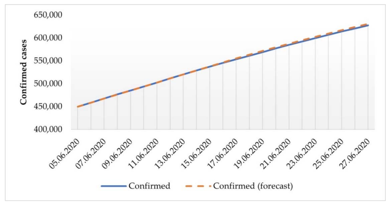
Let us consider the results of applying the developed approach to forecasting the indicators of the epidemic in Russia, for the period from 6 June to 30 June 2020, based on the information available on 5 June 2020.

Figure 2 shows the predicted trajectories built over the period from 6 June to 30 June 2020, which were compared with the actual trajectories. The average deviation of the trajectory of the total number of cases forecasted compared to the actual one was 0.37%. On 30 June 2020, the deviation was found to be minus 1.17%.

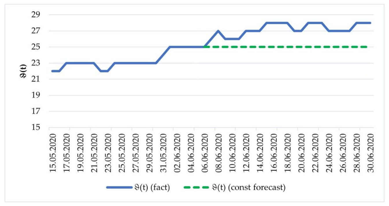
The dynamics of the function $\vartheta \left(t\right)$ for the period under consideration are shown in Figure 3.

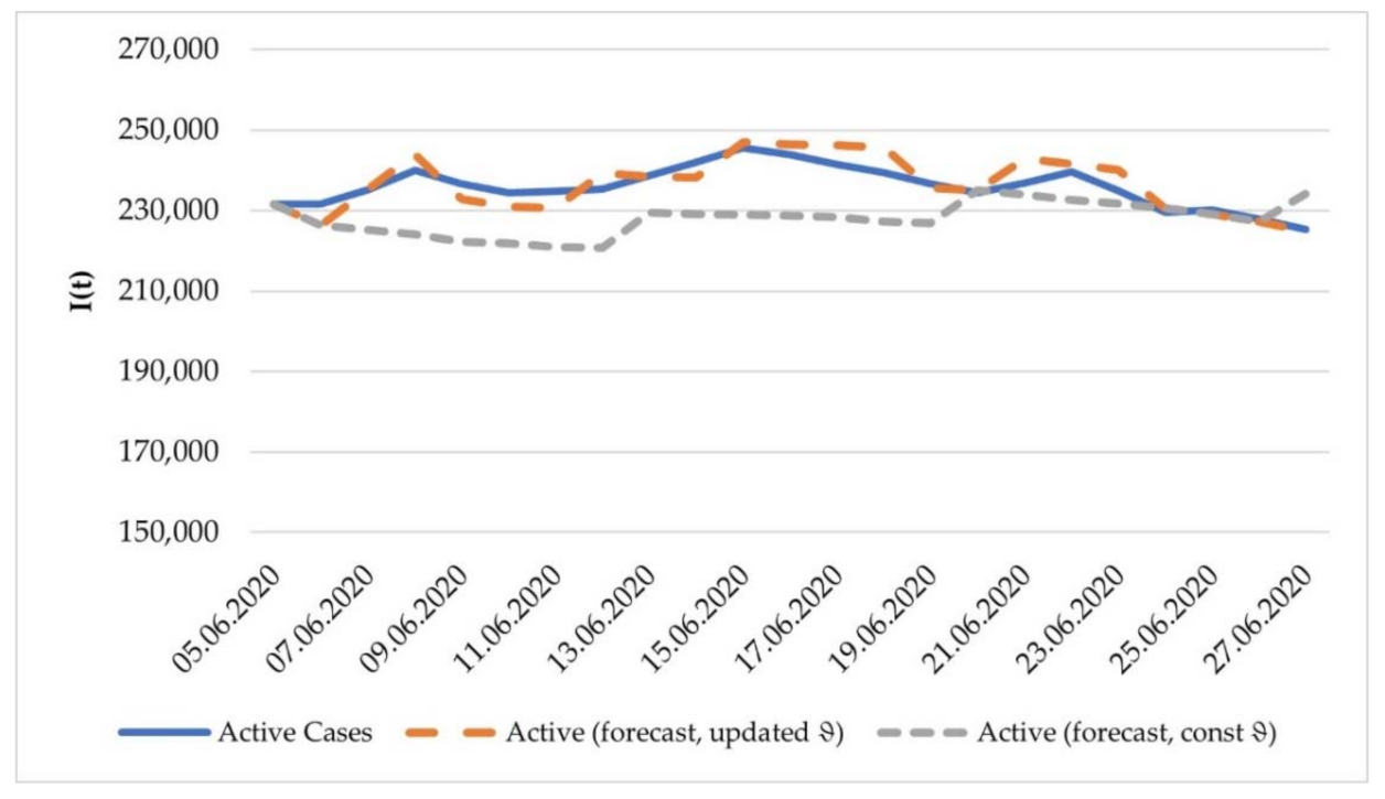
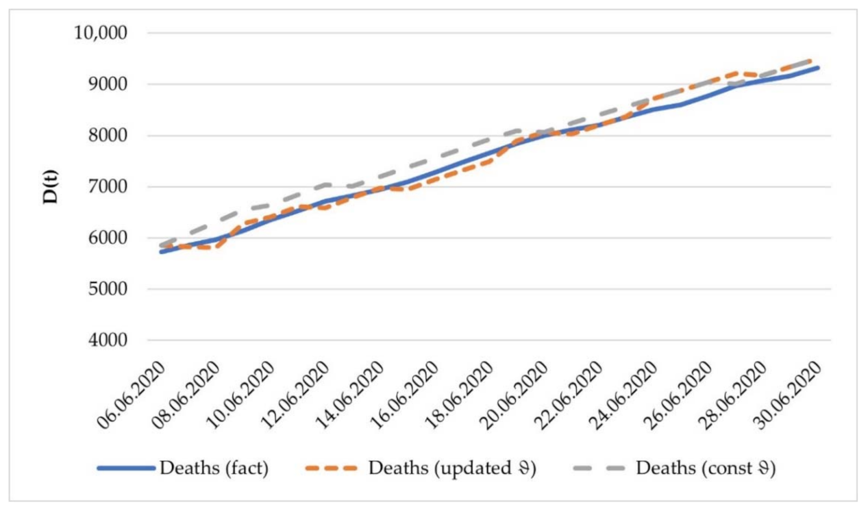
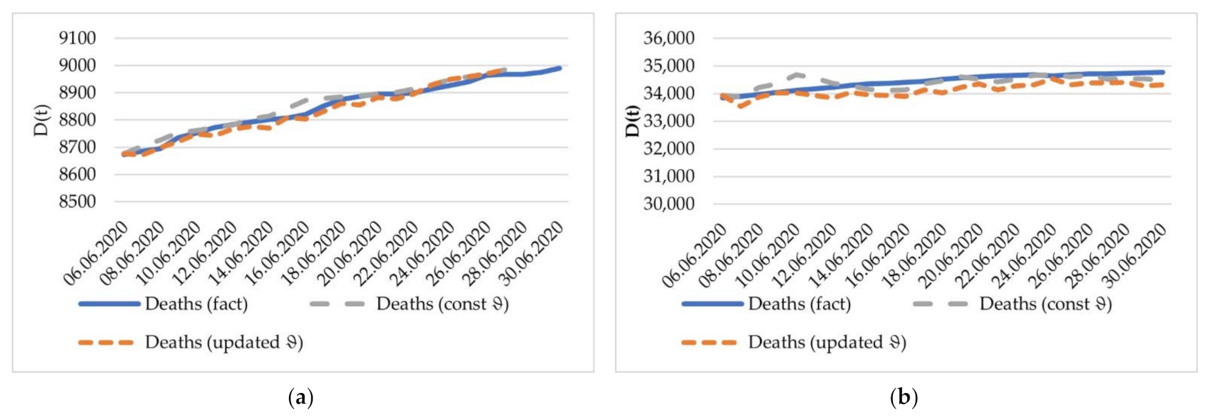
Assuming the stationarity of the epidemiological process from 6 June to 30 June 2020, a constant value of the dynamic balance characteristic corresponding to the actual value at the beginning of the forecasting horizon (25 days) was taken for the calculation. The graphs of the calculated and actual values of the total number of deaths $D\left(t\right)$ and active cases $I\left(t\right)$ are shown in Figure 4 and Figure 5.

The deviation of the modeled trajectory from the actual trajectory of the number of active patients was, on average, 3.63%. The mean absolute percentage error (MAPE) value for this forecast was 4.14%. For the dynamics of the number of deaths, the forecasted MAPE of the considered interval was 3.17%. The maximum deviation was 6.5%.

By using the actual values of $\vartheta \left(t\right)$, the graphs of the actual and predicted values of $D\left(t\right)$ practically coincide. Similarly, the graphs of the total number of active patients in the case of using the actual $\vartheta \left(t\right)$ values practically coincide. In the interval from 6 June to 30 June 2020, the deviation from the actual trajectory of the number of active patients averaged to 1.13% and the number of deaths was 0.4%.

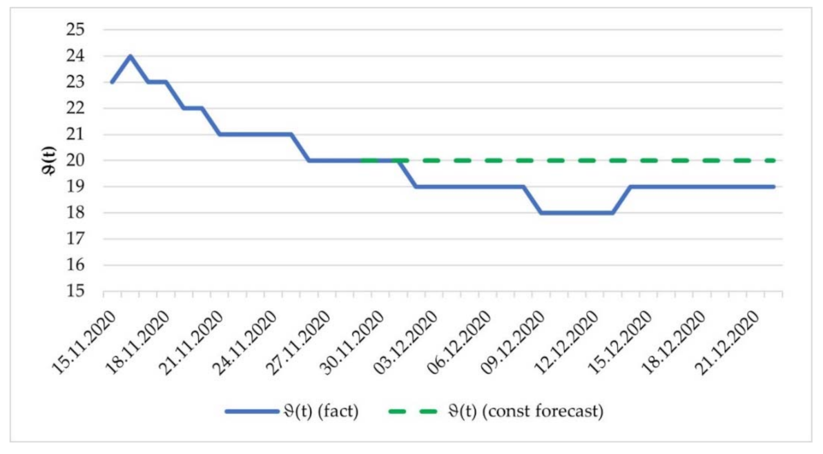
Let us consider the results of applying the developed approach to forecasting the indicators of the epidemic in Russia in the period from 29 November to 22 December 2020, based on the information available on 28 November. Assuming the stationarity of the epidemiological process, the theta value taken was equal to 20. The change of the function $\vartheta \left(t\right)$ over the considered time interval is shown in Figure 6.

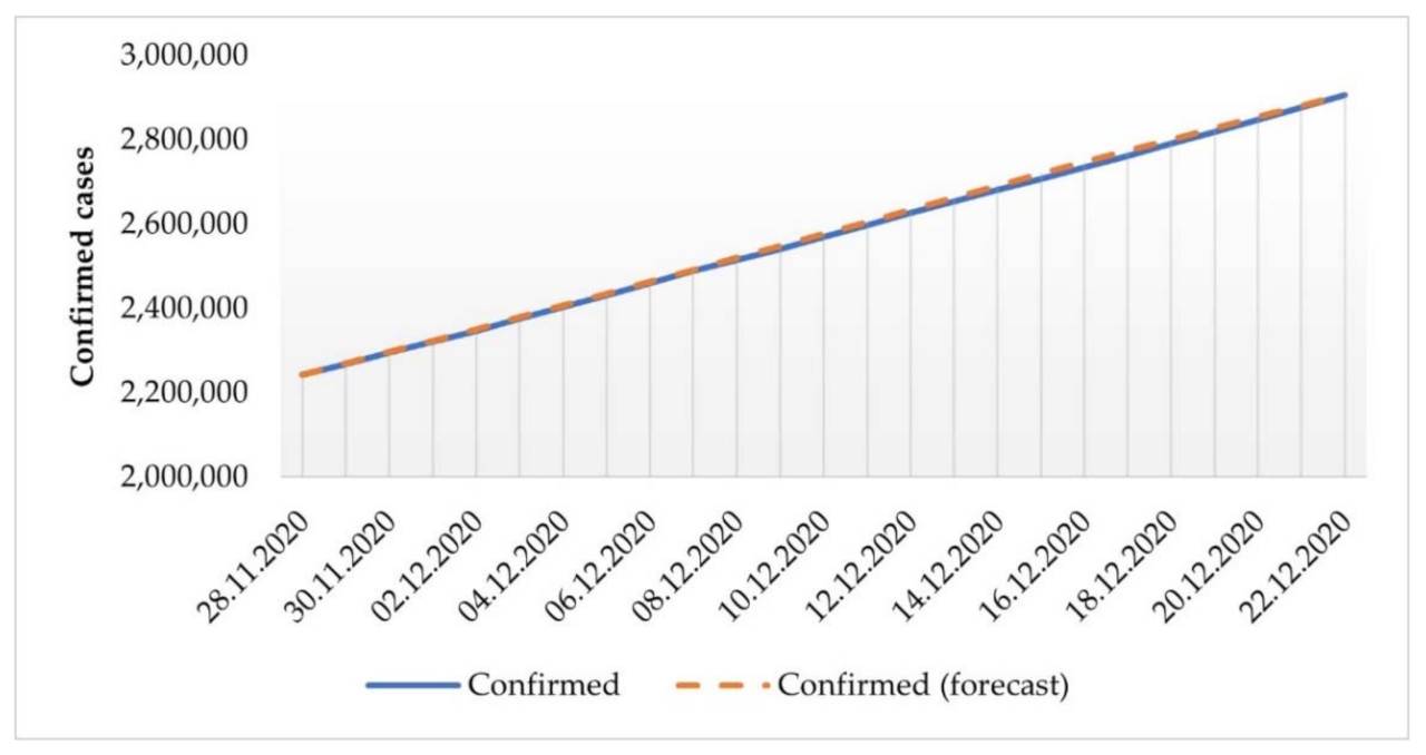
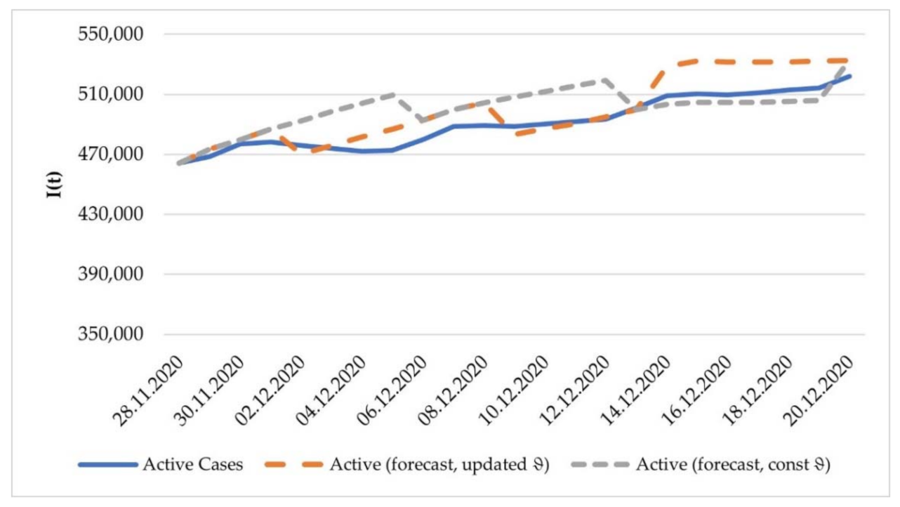
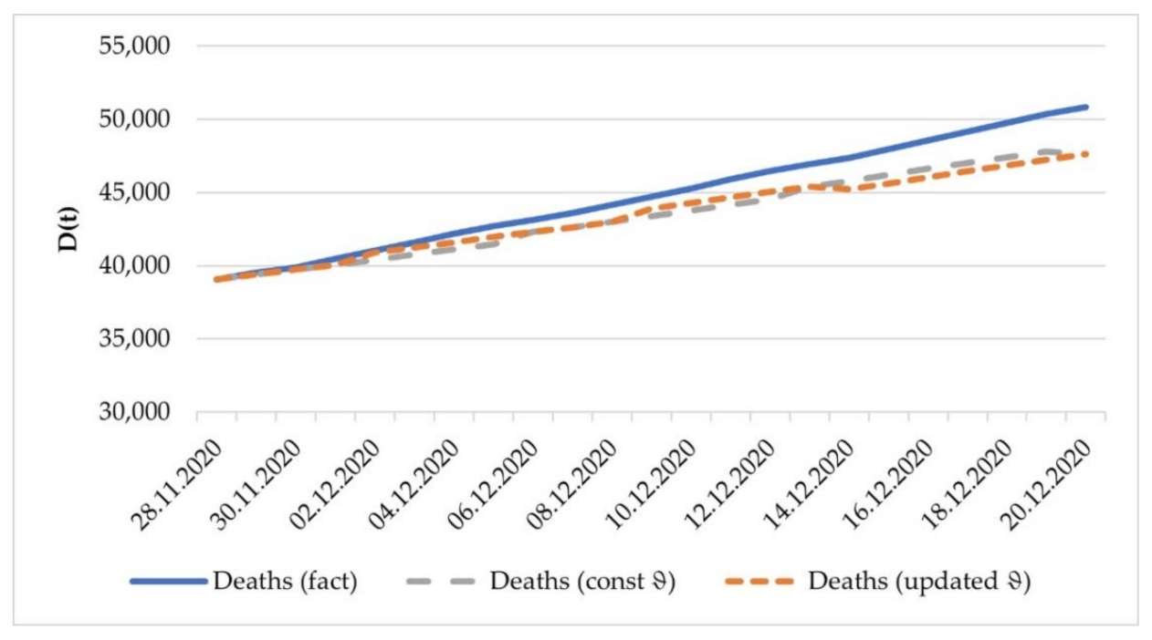
The dynamics of the modeled and actual values of the total number of confirmed cases $C\left(t\right)$, deaths $D\left(t\right)$ and active cases $I\left(t\right)$ are shown in Figure 7, Figure 8 and Figure 9.

The deviation of the modeled trajectory from the actual trajectory of the number of active patients in terms of MAPE was 1.1%. For the dynamics of the predicted trajectory of the deceased, the forecasted MAPE of the considered interval was 3.1%. However, by taking into account the update in information about the dynamic balance characteristic, the deviations of the actual graphs from the predicted values of both I(t) and D(t) decreased. Thus, in the considered interval, the deviation from the actual trajectory of the number of active patients in terms of MAPE was 0.9% and the number of deaths was 2.9%.

4.1.2. Case of Europe

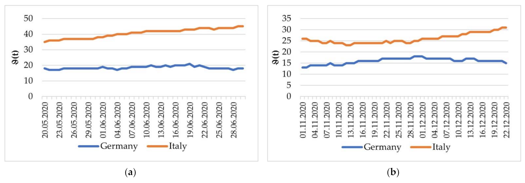
Let us consider the possibilities of applying this approach in other countries. For consistency, similar forecasting time intervals were analyzed. The daily updated statistical data published on the Johns Hopkins University portal were used as the initial information for modeling [56]. The dynamics of $\vartheta \left(t\right)$ are shown in Figure 10.

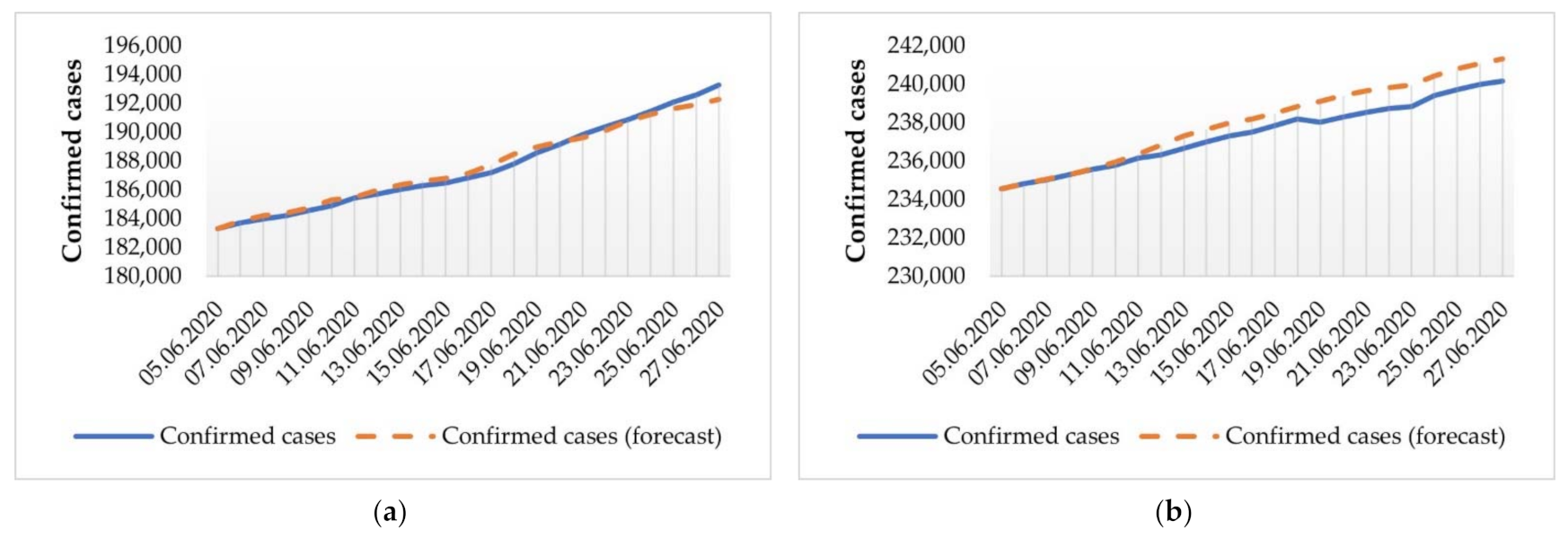
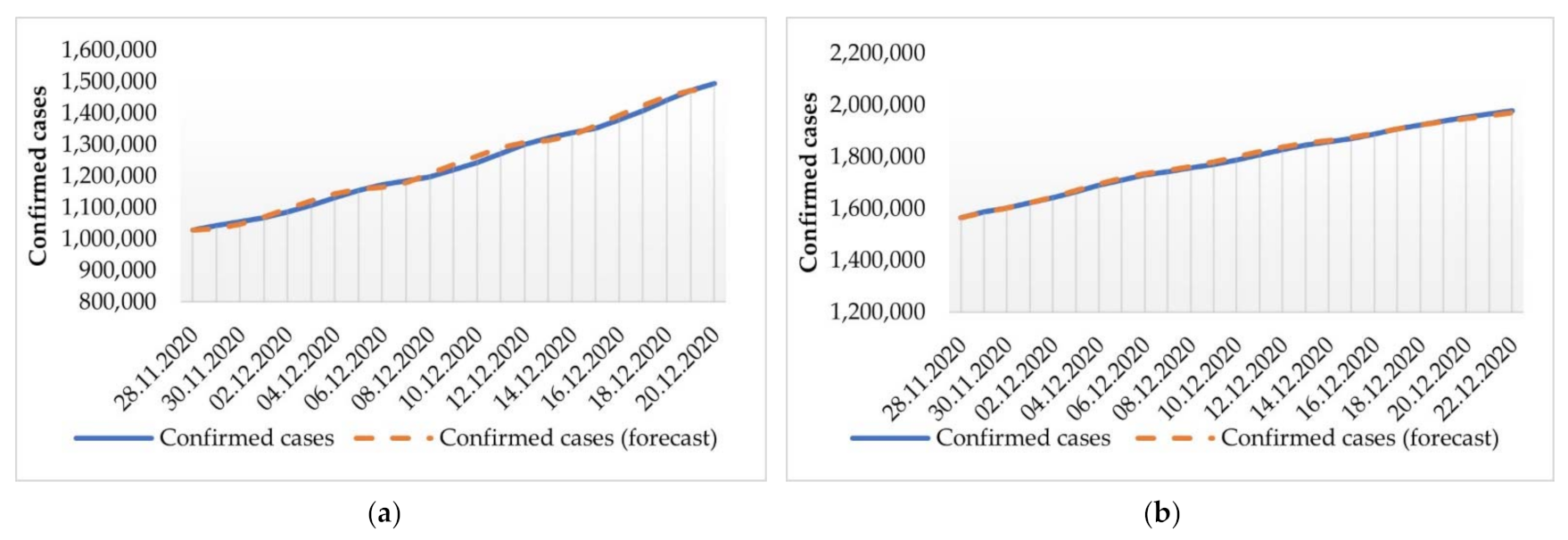
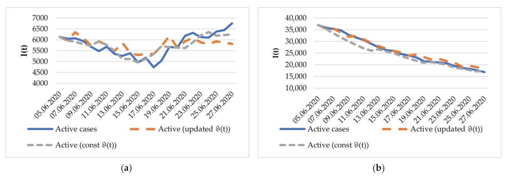
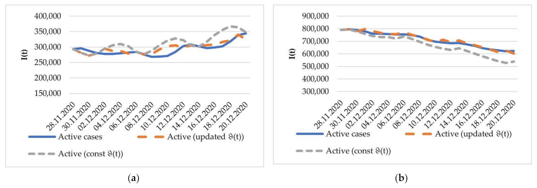
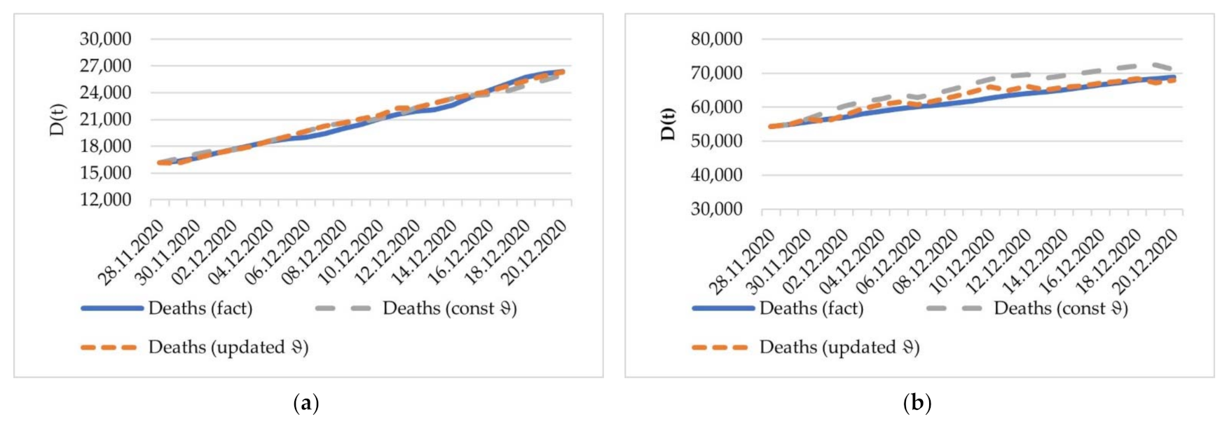
Under the assumption of the piecewise stationarity of the epidemiological process, a constant value of the dynamic balance characteristic corresponding to the actual value at the beginning of the forecasting horizon was used. The case of the dynamic updating of information when the value of the characteristic was updated was also considered. The modeling was carried out at the same time as the intervals that were used to analyze the situation in Russia. The graphs of the modeled and actual values of the total number of confirmed cases, the number of deaths $D\left(t\right)$ and active cases $I\left(t\right)$ are shown in Figure 11, Figure 12, Figure 13, Figure 14, Figure 15 and Figure 16.

For Germany, the value of $\vartheta \left(t\right)=18$ days was used in the summer 2020 forecast. In the winter 2020 case, the $\vartheta \left(t\right)$ value was 17 days. The deviation of the predicted trajectory of the number of active cases in summer was 3.22% in terms of the MAPE indicator. When we used the dynamically updated $\vartheta \left(t\right)$, the MAPE value dropped to 2.8%. When assessing the dynamics of epidemic indicators in December 2020, the MAPE for the trajectory of active infections was 2.7%. When the information was dynamically updated and actual theta values were used, the variance was reduced to 1.25%. The deviation in the total number of cases at both prediction intervals did not exceed 0.25%. For the dynamics of the total number of deaths, the forecast MAPE of the intervals under consideration was 0.7%.

In the case of Italy, the value of $\vartheta \left(t\right)=40$ days was used when constructing the forecast in summer. In winter, the value of $\vartheta \left(t\right)$ was 25 days. The deviation of the number of active cases in the interval from 6 June to 30 June 2020 was 3.85% (3.3% in the case of a dynamic update of information about the $\vartheta \left(t\right)$ value). When assessing the dynamics of epidemic indicators in December 2020, the MAPE for the estimated trajectory of active infections was 9%. When the information was dynamically updated and actual theta values were used, the variance was reduced to 0.5%. The deviation of the total number of cases at both prediction intervals did not exceed 0.1%. For the dynamics of the total number of deaths, the forecast MAPE of the intervals under consideration did not exceed 5.7%. Summary results of the assessment of forecast accuracy in terms of MAPE are presented in

Table 2. Forecast results for the constant and dynamically updated $\vartheta \left(t\right)$.

Country	$\mathit{\vartheta }\left(\mathit{t}\right)$	C(t) Forecast (MAPE)	Constant ϑ(t)		$\mathbf{Dynamically} \mathbf{Updated} \mathit{\vartheta }\left(\mathit{t}\right)$
			I(t) Forecast (MAPE)	D(t) Forecast (MAPE)	I(t) Forecast (MAPE)	D(t) Forecast (MAPE)
6–30 June 2020
Russia	25	0.37%	4.14%	3.17%	1.13%	0.4%
Germany	18	0.25%	3.22%	0.7%	2.8%	0.7%
Italy	40	0.1%	3.85%	5.7%	3.3%	5.7%
1–20 December 2020
Russia	20	0.30%	1.10%	3.10%	0.9%	2.9%
Germany	17	0.25%	2.70%	0.7%	1.25%	0.7%
Italy	25	0.10%	9%	5.7%	0.5%	5.7%

.

Based on [58], we described an example of using the SIR model for forecasting the dynamics of active cases in Russia during the period from 20 April 2020 to 19 May 2020. The results of the I(t) forecasts using the SIR and CIRD models are presented in

Table 3. The $I\left(t\right)$ forecast results for the SIR and CIRD models, for the period from 20 April 2020 to 19 May 2020, in Russia.

Data	Actual I(t)	I(t) Forecast, SIR	I(t) Forecast, CIRD	SIR Difference	CIRD Difference
20 April 20	43,270	43,270		0
21 April 20	48,434	46,332		−2102
22 April 20	53,066	49,612	53,268	−3454	−202
23 April 20	57,327	53,122	58,366	−4205	−1039
24 April 20	62,421	56,881	63,526	−5540	−1105
25 April 20	67,657	60,906	68,840	−6751	−1183
26 April 20	73,435	65,215	75,652	−8220	−2217
27 April 20	79,007	69,828	81,619	−9179	−2612
28 April 20	84,235	74,767	87,616	−9468	−3381
29 April 20	88,138	80,055	93,575	−8083	−5437
30 April 20	93,806	85,716	101,582	−8090	−7776
01 May 20	100,042	91,777	108,151	−8265	−8109
02 May 20	107,819	98,265	114,394	−9554	−6575
03 May 20	116,768	105,211	120,414	−11,557	−3646
04 May 20	125,817	112647	129,095	−13,170	−3278
05 May 20	134,054	120,607	135,054	−13,447	−1000
06 May 20	143,065	129,128	140,395	−13,937	2670
07 May 20	151,732	138,249	149,063	−13,483	2669
08 May 20	159,528	148,012	154,160	−11,516	5368
09 May 20	164,933	158,462	158,861	−6471	6072
10 May 20	173,467	169,647	163,065	−3820	10,402
11 May 20	179,534	181,619	166,203	2085	13,331
12 May 20	186,615	194,432	171,332	7817	15,283
13 May 20	192,056	208,144	175,275	16,088	16,781
14 May 20	196,410	222,819	179,801	26,409	16,609
15 May 20	202,199	238,524	184,952	36,325	17,247
16 May 20	206,304	255,329	189,177	49,025	17,127
17 May 20	211,748	273,311	193,418	61,563	18,330
18 May 20	217,747	292,551	197,381	74,804	20,366
19 May 20	220,974	313,136	201,606	92,162	19,368

. It contains information on real data of the I(t) dynamics, the forecasted trajectories based on the SIR and CIRD models, as well as the deviations of the predicted values from the real ones in the form of differences in values. The forecast MAPE for the trajectory of the active cases using the SIR model was 11%, while the application of the proposed technique based on the principle of dynamic balance gave a value of 1.85% MAPE for the same time period.

5. Discussion and Conclusions

The present study focused on the possibilities of analyzing the dynamics of changes in the indicators of the spread of the COVID-19 during the first wave of epidemic. A distinctive feature of such periods is the lack of sufficient statistics. On the other hand, vaccination had not yet been initiated, so everyone could be considered as having been a potential patient. Percentage growth was used as the most important parameter of the model, which has a stochastic nature. Another important result of the study was the description of the principle of dynamic balance of epidemiological processes previously not used by other researchers to model epidemics. The principle lies in the fact that the past values of the total number of cases are close enough to the values of the total number of recovered and deceased patients at the current time. At the same time, the time intervals through which such a balance is observed change in time rather predictably, although like the percentage increase, they take random values. This study considered the case when the dynamic balance characteristic was constant during the forecasting horizon.

Following the proposed approach for choosing the parameters of epidemic modeling, this paper presented a new discrete CIRD model of the epidemic spread, which uses random values of the percentage increase and characteristics of the dynamic balance to describe the dynamics of the total number of cases, the total number of recovered and deaths, and the number of active cases of the disease. To predict the values of the total number of cases, the CBRR model was used, which was previously proposed and tested by the authors. It first predicts the percentage increase in the total number of cases in the medium term using the precedent method and intelligent algorithms for extracting the necessary data using a special class of the predictive dynamic regression model (PDRM) model [58], and then uses the obtained values to predict the total number of confirmed cases. The forecasting horizon of the CIRD model, as a rule, is limited by a value equal to the value of the dynamic balance characteristic of the epidemic, calculated on the basis of the principle of dynamic balance of the epidemiological processes formulated in Theorem 1. Since the characteristic of the dynamic balance is a random variable that depends on time and takes integer values, the possibilities for using the CIRD model to predict the dynamics of non-stationary epidemiological processes are still limited. However, as the calculations show, the forecasting accuracy when using the proposed model, even in the case of the non-stationarity of epidemiological processes in the forecasting interval, is quite high (see Figure 11, Figure 12, Figure 13, Figure 14, Figure 15 and Figure 16). For example, when predicting the dynamics of active cases of the disease, MAPE deviations in Germany ranged from 2.7% to 3.2%, in Italy, from 3.8% to 9%, and in Russia, from 1.1% to 4.1%. At the same time, the MAPE indicator for predicting the dynamics of deaths did not exceed 5.7% for all countries and time intervals considered.

References

- World Health Organization. Available online: https://search.bvsalud.org/global-literature-on-novel-coronavirus-2019-ncov/ (accessed on 15 December 2021).
- Shinde, G.R.; Kalamkar, A.B.; Mahalle, P.N.; Dey, N.; Chaki, J.; Hassanien, A.E. Forecasting Models for Coronavirus (COVID-19): A Survey of the State-of-the-Art. SN Comput. Sci. 2020, 1, 197. [Google Scholar] [CrossRef]
- Moftakhar, L.; Seif, M.; Safe, M.S. Exponentially increasing trend of infected patients with COVID-19 in Iran: A comparison of neural network and ARIMA forecasting models. Iran. J. Public Health 2020, 49, 92–100. [Google Scholar] [CrossRef]
- Singh, S.; Chowdhury, C.; Panja, A.K.; Neogy, S. Time Series Analysis of COVID-19 Data to Study the Effect of Lockdown and Unlock in India. J. Inst. Eng. India Ser. B 2021, 102, 1275–1281. [Google Scholar] [CrossRef]
- Harvey, A.; Kattuman, P. A farewell to R: Time-series models for tracking and forecasting epidemics. J. R. Soc. Interface 2021, 18, 20210179. [Google Scholar] [CrossRef]
- Aditya Satrio, C.B.; Darmawan, W.; Nadia, B.U.; Hanafiah, N. Time series analysis and forecasting of coronavirus disease in Indonesia using ARIMA model and PROPHET. Procedia Comput. Sci. 2021, 179, 524–532. [Google Scholar] [CrossRef]
- Chen, S.; Robinson, P.; Janies, D.; Dulin, M. Four Challenges Associated with Current Mathematical Modeling Paradigm of Infectious Diseases and Call for a Shift. Open Forum Infect. Dis. 2020, 7, ofaa333. [Google Scholar] [CrossRef] [PubMed]
- Kermack, W.O.; McKendrick, A.G. A contribution to the mathematical theory of epidemics. Proc. R. Soc. Lond. Ser. A 1927, 115, 700–721. [Google Scholar] [CrossRef] [Green Version]
- Anderson, R.M.; May, R.M. Infectious Diseases of Humans: Dynamics and Control; Oxford University Press: Oxford, UK, 1991. [Google Scholar]
- Dil, S.; Dil, N.; Maken, Z.H. COVID-19 Trends and Forecast in the Eastern Mediterranean Region with a particular focus on Pakistan. Cureus 2020, 12, e8582. [Google Scholar] [CrossRef] [PubMed]
- Rodrigues, H.S. Application of SIR epidemiological model: New trends. Int. J. Appl. Math. Inform. 2016, 10, 92–97. [Google Scholar] [CrossRef]
- Iwami, S.; Takeuchi, Y.; Liu, X. Avian–human influenza epidemic model. Math. Biosci. 2007, 207, 1–25. [Google Scholar] [CrossRef]
- Teles, P. Predicting the evolution of SARS-COVID-2 in Portugal using an adapted SIR model previously used in South Korea for the MERS outbreak. MedRxiv 2020. [Google Scholar] [CrossRef]
- Rǎdulescu, A.; Williams, C.; Cavanagh, K. Management strategies in a SEIR-type model of COVID 19 community spread. Sci. Rep. 2020, 10, 21256. [Google Scholar] [CrossRef] [PubMed]
- Fanelli, D.; Piazza, F. Analysis and forecast of COVID-19 spreading in China, Italy and France. Chaos Solitons Fractals 2020, 134, 109761. [Google Scholar] [CrossRef]
- Zhao, C.; Tepekule, B.; Criscuolo, N.G.; Wendel, G.P.; Hilty, M.P.; RISC-ICU Consortium Investigators in Switzerland; Fumeaux, T.; Van Boeckel, T. Icumonitoring.ch: A platform for short-term forecasting of intensive care unit occupancy during the COVID-19 epidemic in Switzerland. Swiss Med. Wkly. 2020, 150, w20277. [Google Scholar] [CrossRef]
- Chinazzi, M.; Davis, J.T.; Ajelli, M.; Gioannini, C.; Litvinova, M.; Merler, S.; Pastore, Y.; Piontti, A.; Mu, K.; Rossi, L.; et al. The effect of travel restrictions on the spread of the 2019 novel coronavirus (COVID-19) outbreak. Science 2020, 368, 395–400. [Google Scholar] [CrossRef] [Green Version]
- Tang, B.; Wang, X.; Li, Q.; Bragazzi, N.L.; Tang, S.; Xiao, Y.; Wu, J. Estimation of the transmission risk of 2019-nCov and its implication for public health interventions. J. Clin. Med. 2020, 9, 462. [Google Scholar] [CrossRef] [PubMed] [Green Version]
- Tian, H.; Liu, Y.; Li, Y. An investigation of transmission control measures during the first 50 days of the COVID-19 epidemic in China. Science 2020, 368, 638–642. [Google Scholar] [CrossRef] [PubMed] [Green Version]
- López, L.; Rodó, X. A modified SEIR model to predict the COVID-19 outbreak in Spain and Italy: Simulating control scenarios and multi-scale epidemics. Results Phys. 2021, 21, 103746. [Google Scholar] [CrossRef] [PubMed]
- Feng, S.; Feng, Z.; Ling, C.; Chang, C.; Feng, Z. Prediction of the COVID-19 epidemic trends based on SEIR and AI models. PLoS ONE 2021, 16, e0245101. [Google Scholar] [CrossRef]
- Matveev, A. The mathematical modeling of the effective measures against the COVID-19 spread. Natl. Secur. Strateg. Plan. 2020, 1, 23–39. [Google Scholar] [CrossRef]
- Anastassopoulou, C.; Russo, L.; Tsakris, A.; Siettos, C. Data-based analysis, modelling and forecasting of the COVID-19 outbreak. PLoS ONE 2020, 15, e0230405. [Google Scholar] [CrossRef] [Green Version]
- Calafiore, G.C.; Novara, C.; Possieri, C. A time-varying SIRD model for the COVID-19 contagion in Italy. Annu. Rev. Control 2020, 50, 361–372. [Google Scholar] [CrossRef]
- Maier, B.F.; Brockmann, D. Effective containment explains subexponential growth in recent confirmed COVID-19 cases in China. Science 2020, 368, 742–746. [Google Scholar] [CrossRef] [PubMed] [Green Version]
- Mandal, S.; Bhatnagar, T.; Arinaminpathy, N. Prudent public health intervention strategies to control the coronavirus disease 2019 transmission in India. A mathematical model-based approach. Indian J. Med. Res. 2020, 151, 190–199. [Google Scholar] [CrossRef] [PubMed]
- Choi, S.; Ki, M. Estimating the reproductive number and the outbreak size of COVID-19 in Korea. Epidemiol. Health 2020, 42, e2020011. [Google Scholar] [CrossRef] [PubMed] [Green Version]
- Guglielmi, N.; Iacomini, E.; Viguerie, A. Delay differential equations for the spatially re-solved simulation of epidemics with specific application to COVID-19. Math. Methods Appl. Sci. 2022, 45, 4752–4771. [Google Scholar] [CrossRef] [PubMed]
- Guglielmi, N.; Elisa Iacomini, E.; Viguerie, A. Identification of Time Delays in COVID-19 Data. arXiv 2021, arXiv:2111.13368. [Google Scholar]
- Pugliese, A.; Sottile, S. Inferring the COVID-19 infection curve in Italy. arXiv 2020, arXiv:2004.09404. [Google Scholar]
- Paul, S.; Lorin, E. Estimation of COVID-19 recovery and decease periods in Canada using delay model. Sci. Rep. 2021, 11, 23763. [Google Scholar] [CrossRef] [PubMed]
- Dell’Anna, L. Solvable delay model for epidemic spreading: The case of Covid-19 in Italy. Sci. Rep. 2020, 10, 15763. [Google Scholar] [CrossRef] [PubMed]
- Yang, C.; Yang, Y.; Li, Z.; Zhang, L. Modeling and analysis of COVID-19 based on a time delay dynamic model. Math. Biosci. Eng. 2021, 18, 154–165. [Google Scholar] [CrossRef]
- Adam, D. Special report: The simulations driving the world’s response to COVID-19. Nature 2020, 580, 316–318. [Google Scholar] [CrossRef]
- Amelin, K.; Granichin, O.; Sergeenko, A.; Volkovich, Z.V. Emergent Intelligence via Self-Organization in a Group of Robotic Devices. Mathematics 2021, 9, 1314. [Google Scholar] [CrossRef]
- Wieczorek, M.; Siłka, J.; Woźniak, M. Neural network powered COVID-19 spread forecasting model. Chaos Solitons Fractals 2020, 140, 110203. [Google Scholar] [CrossRef]
- Liu, D.; Clemente, L.; Poirier, C.; Ding, X.; Chinazzi, M.; Davis, J.; Vespignani, A.; Santillana, M. Real-Time Forecasting of the COVID-19 Outbreak in Chinese Provinces: Machine Learning Approach Using Novel Digital Data and Estimates from Mechanistic Models. J. Med. Internet Res. 2020, 22, e20285. [Google Scholar] [CrossRef]
- Kumar, R.L.; Khan, F.; Din, S.; Band, S.S.; Mosavi, A.; Ibeke, E. Recurrent Neural Network and Reinforcement Learning Model for COVID-19 Prediction. Front. Public Health 2021, 9, 744100. [Google Scholar] [CrossRef]
- Ayoobi, N.; Sharifrazi, D.; Alizadehsani, R.; Shoeibi, A.; Gorriz, J.M.; Moosaei, H.; Khosravi, A.; Nahavandi, S.; Gholamzadeh Chofreh, A.; Goni, F.A.; et al. Time series forecasting of new cases and new deaths rate for COVID-19 using deep learning methods. Results Phys. 2021, 27, 104495. [Google Scholar] [CrossRef]
- Alali, Y.; Harrou, F.; Sun, Y. A proficient approach to forecast COVID-19 spread via optimized dynamic machine learning models. Sci. Rep. 2022, 12, 2467. [Google Scholar] [CrossRef]
- Zhao, H.; Merchant, N.N.; McNulty, A.; Radcliff, T.A.; Cote, M.J.; Fischer, R.S.B.; Sang, H.; Ory, M.G. COVID-19: Short term prediction model using daily incidence data. PLoS ONE 2021, 16, e0250110. [Google Scholar] [CrossRef]
- Amaral, F.; Casaca, W.; Oishi, C.M.; Cuminato, J.A. Towards Providing Effective Data-Driven Responses to Predict the COVID-19 in São Paulo and Brazil. Sensors 2021, 21, 540. [Google Scholar] [CrossRef]
- Pavlyutin, M.; Samoyavcheva, M.; Kochkarov, R.; Pleshakova, E.; Korchagin, S.; Gataullin, T.; Nikitin, P.; Hidirova, M. COVID-19 Spread Forecasting, Mathematical Methods vs. Machine Learning, Moscow Case. Mathematics 2022, 10, 195. [Google Scholar] [CrossRef]
- Katris, C. A time series-based statistical approach for outbreak spread forecasting: Application of COVID-19 in Greece. Expert Syst. Appl. 2021, 166, 114077. [Google Scholar] [CrossRef]
- Finkenstädt, B.F.; Grenfell, B.T. Time series modelling of childhood diseases: A dynamical systems approach. J. R. Stat. Soc. Ser. C (Appl. Stat.) 2000, 49, 187–205. [Google Scholar] [CrossRef]
- Kondratyev, M. Forecasting methods and models of disease spread. Comput. Res. Modeling 2013, 5, 863–882. [Google Scholar] [CrossRef] [Green Version]
- Zakharov, V.; Balykina, Y.; Petrosian, O.; Gao, H. CBRR Model for Predicting the Dynamics of the COVID-19 Epidemic in Real Time. Mathematics 2020, 8, 1727. [Google Scholar] [CrossRef]
- Zakharov, V.; Balykina, Y. Predicting the dynamics of the coronavirus (COVID-19) epidemic based on the case-based reasoning approach. Vestn. St.-Peterbg. Univ. Appl. Math. Comput. Sci. Control Process 2020, 16, 249–259. [Google Scholar] [CrossRef]
- Dairi, A.; Harrou, F.; Zeroual, A.; Hittawe, M.M.; Sun, Y. Comparative study of machine learning methods for COVID-19 transmission forecasting. J. Biomed. Inform. 2021, 18, 103791. [Google Scholar] [CrossRef]
- CDC. Reported and Forecasted New and Total COVID-19 Deaths in USA. Available online: https://www.cdc.gov/coronavirus/2019-ncov/science/forecasting/forecasting-us.html (accessed on 7 December 2021).
- Congdon, P. Mid-Epidemic Forecasts of COVID-19 Cases and Deaths: A Bivariate Model Applied to the UK. Interdiscip. Perspect. Infect. Dis. 2021, 2021, 8847116. [Google Scholar] [CrossRef]
- Banoei, M.M.; Dinparastisaleh, R.; Zadeh, A.V.; Mirsaeidi, M. Machine-learning-based COVID-19 mortality prediction model and identification of patients at low and high risk of dying. Crit. Care 2021, 25, 328. [Google Scholar] [CrossRef]
- Ahmadini, A.A.H.; Naeem, M.; Aamir, M.; Dewan, R.; Alshqaq, S.S.A.; Mashwani, W.K. Analysis and Forecast of the Number of Deaths, Recovered Cases, and Confirmed Cases from COVID-19 for the Top Four Affected Countries Using Kalman Filter. Front. Phys. 2021, 9, 629320. [Google Scholar] [CrossRef]
- Ioannidis, J.; Cripps, S.; Tanner, M.A. Forecasting for COVID-19 has failed. Int. J. Forecast. 2020. advance online publication. [Google Scholar] [CrossRef] [PubMed]
- Hasan, M.N.; Haider, N.; Stigler, F.L.; Khan, R.A.; McCoy, D.; Zumla, A.; Kock, R.A.; Uddin, M.J. The Global Case-Fatality Rate of COVID-19 Has Been Declining Since May 2020. Am. J. Trop. Med. Hyg. 2021, 104, 2176–2184. [Google Scholar] [CrossRef] [PubMed]
- Johns Hopkins Coronavirus Resource Center. Available online: https://coronavirus.jhu.edu/map.html (accessed on 15 December 2021).
- Chaudhry, R.M.; Hanif, A.; Chaudhary, M.; Minhas, S., II; Mirza, K.; Asif, T.; Gilani, S.A.; Kashif, M. Coronavirus disease 2019 (COVID-19): Forecast of an emerging urgency in Pakistan. Cureus 2020, 12, e8346. [Google Scholar] [CrossRef] [PubMed]
- Zakharov, V.; Balykina, Y. Balance Model of COVID-19 Epidemic Based on Percentage Growth Rate. Inform. Autom. 2021, 20, 1034–1064. [Google Scholar] [CrossRef]
- Izvestia Newspaper. Available online: https://iz.ru/1233744/olga-kolentcova/podem-s-povorotom-matematiki-dali-novyi-prognoz-po-zabolevaemosti-covid (accessed on 15 December 2021).
- Center for Intelligent Logistics of St. Petersburg State University. Available online: http://old.apmath.spbu.ru/cil/index_en.html (accessed on 12 December 2021).
Figure 1.
dynamics for Russia, Germany and Italy during the time period of May to December 2020.
Figure 2.
Dynamics of the total number of , the actual and predicted trajectories.
Figure 3.
Actual and modeled values of the dynamic balance characteristic from 15 May to 30 June 2022.
Figure 4.
Dynamics of , the actual and modeled trajectories in the interval from 6 June to 30 June 2020.
Figure 5.
Dynamics of , the actual and calculated trajectories in the interval from 6 June to 30 June 2020 in a stationary case and in the case of updated values of .
Figure 6.
Actual and modeled values of the dynamic balance characteristic from 15 November to 30 December 2020.
Figure 7.
Dynamics of , the actual and modeled trajectories in the interval from 1 December to 22 December 2020.
Figure 8.
Dynamics of , the actual and modeled trajectories in the interval from 1 December to 22 December 2020, in a stationary case and at updated values of .
Figure 9.
Figure 10.
Dynamics of changes in the values of in Germany and Italy (a) from May to June 2020 and (b) from November to December 2020.
Figure 11.
Dynamics of , the actual and modeled trajectories in the interval, from 6 June to 30 June 2020, in (a) Germany and (b) Italy.
Figure 12.
Dynamics of , the actual and modeled trajectories in December 2020, in (a) Germany and (b) Italy.
Figure 13.
Figure 14.
Dynamics of , the actual and calculated trajectories for the interval of 1 to 20 December 2020, in a stationary case and with the updated values of , in (a) Germany and (b) Italy.
Figure 15.
Dynamics of , the actual and calculated trajectories in the interval from 6 June to 30 June 2020, in a stationary case and with the updated values of , in (a) Germany and (b) Italy.
Figure 16.