Electricity Demand Elasticity, Mobility, and COVID-19 Contagion Nexus in the Italian Day-Ahead Electricity Market

Abstract

The magnitude of the impact of the pandemic on key variables, such as electricity demand, mobility of people and number of COVID-19 hospitalization cases, has been unprecedented. Existing economic models have not estimated the impact of sucokh events. This paper fills this gap, investigating the nexus among electricity demand elasticity, shifting behaviors of mobility and COVID-19 contagion with econometric estimation techniques. Firstly, using the single bids to purchase recorded in the Italian day-ahead wholesale electricity market in 2020, we estimate hourly electricity demand and price elasticity directly from short-run consumer behavior. Then, we analyze the effects of the main aspects of the pandemic, the health situation and the mobility contraction at the national level, on the estimated price elasticities. The period of heavy lockdown between 10 March and 3 June recorded a reduction in the price elasticity of electricity demand. However, when the pandemic broke out again at the beginning of October, elasticity increased, highlighting how companies and economic activities had adopted countermeasures to avoid the arrest of the economy and, consequently, the sharp contraction in electricity demand.

1. Introduction

The COVID-19 pandemic, triggered by a novel coronavirus, broke out at the beginning of 2020. The world observed a global lockdown due to the new virus outbreak. The World Health Organization declared it a pandemic on 12 March 2020.

The pandemic has significantly impacted the economy, society and people’s daily lives. Maintaining social distancing was the best approach to minimize the spread of the virus, and governments worldwide were compelled to take various actions to contain the threat of coronavirus, including lockdowns, factory closedowns and travel bans. These restrictions have greatly changed people’s working patterns and lifestyles and thus, have resulted in a significant change in electricity demand loads, profiles and composition [1,2,3]. Due to restriction policies, industry and business operations slowed down and, in turn, industrial and commercial electricity loads decreased. As people were forced to stay home, residential electricity demand rose dramatically.

Ref. [1] compared the changes in electricity consumption among different European countries according to the different degrees of stringency of the lockdown policies. Ref. [2] focused on the Jordan electricity sector and confirmed the increase in the share of residential consumption and the decrease in the share of the commercial sector. Ref. [3] pointed out instead a minimal decrease in the electricity profile of the United Arab Emirates, where only composition changed, with an increase in residential share and a decrease in the shares of the commercial, industrial, and agricultural sectors.

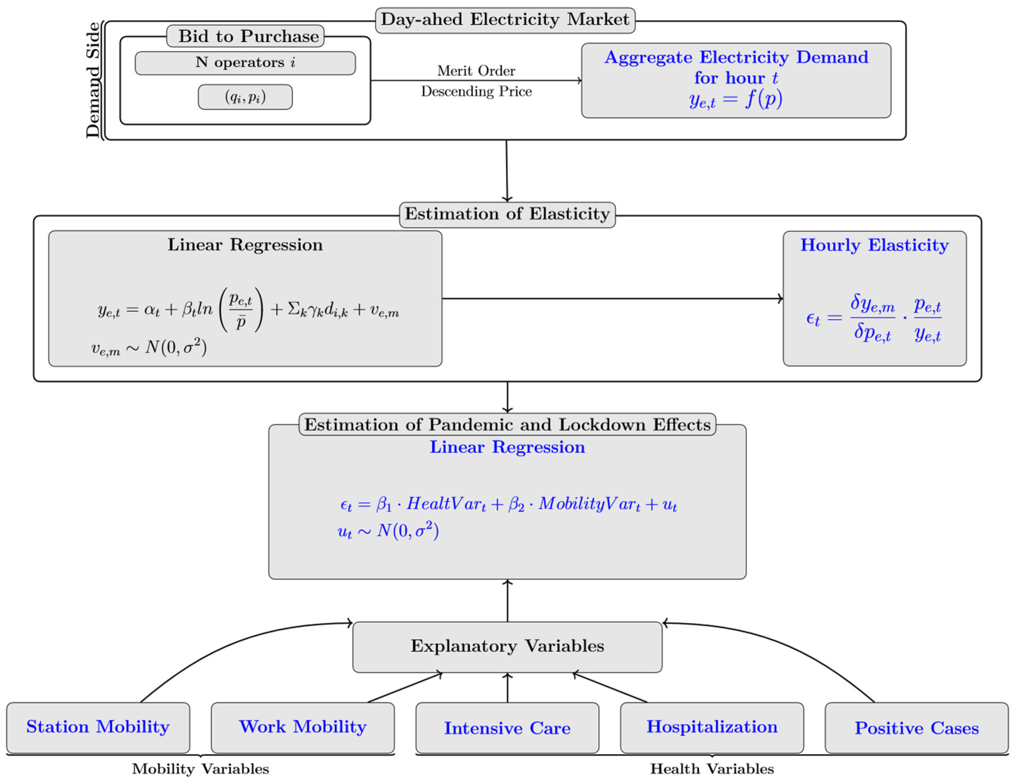
In this study we focus on the Italian case and we scrutinize the impact of the COVID-19 pandemic shock on the price responsiveness of Italian electricity demand, to help researchers, managers and policymakers better understand the implications of the pandemic on the electricity industry. Firstly, we construct a theoretical behavioral model of electricity demand in the Italian market; secondly, we estimate the hourly electricity demand using the bid data collected in the Italian day-ahead wholesale electricity market. Lastly, we measure price elasticity, directly from short-run consumer behavior, and analyze the effects of the main determinants of the pandemic on the price responsiveness. In Figure 1 we show the flow chart summarizing the main steps undertaken in the analysis.

The pandemic has affected the electricity industry through various sources (from the global energy markets to the residential sector) and induced policymakers to enact new measures [4].

Halted industrial operation and restricted business due to the travel ban and lack of workforce resulted in the crash of the global stock market, which shrank by more than 25% in March 2020. The international oil price dropped in March 2020 to the lowest level since 2003 due to the combined effects of COVID-19-related demand drops and business issues among Saudi Arabia, the USA and Russia [5].

Some authors have analyzed the impact of the COVID-19 containment policies on one of the most affected sectors, i.e., the transport sector, especially the aviation industry [6,7,8,9] pointed out that the shrinkage of electricity demand was related to public transport; in China, the UK and the USA, public transport declined by 70% to 90%, depending on city and route. Since in many countries a significant part of public transport is electrical such as trams, trains and public vehicles, the decreased traffic impacted the electricity demand from the transport sector.

Ref. [7] focused on global mobility trends in response to the COVID-19 pandemic and analyzed the crisis-induced changes in mobility behavior and the global implications from a greenhouse gas emissions perspective in Canada. Results showed substantial energy savings and GHG reductions associated with the pandemic. Other authors [8,9] have focused on the positive effect on the environment in terms of emission reduction. Ref. [8] observed that, during the lockdown period, the CO₂ concentration reduced by 35.7% in China. Ref. [9] showed that in April 2020 CO₂ and NOx from the electricity sector declined by 18% and 22%, respectively. In this paper we focus on the crisis-induced changes in consumer behaviors in purchasing electricity by estimating the price responsiveness of electricity demand.

The following scenarios have occurred in the power system due to the COVID-19 outbreak and the restriction policies. Firstly, the downturn in the economy resulted inevitably in a significant drop in the daily average load demand. In China (where the outbreak of the pandemic started earlier) total electricity demand in January and February 2020 was 8% less than the 2019 demand during the same period. In Australia, the overall electricity demand was down by 6.7% in March, as shown by [10]. In France, the power sector faced an approximately 70% revenue loss in March 2020 compared to March 2019 [11]. In Spain the power demand decreased by 3% in March 2020 and 24% in April 2020 compared to the same period in 2019, while in the UK electricity demand in the third week of March 2020 decreased by 6% compared to the first week of March 2020 [12]. In this study we show the downturn in electricity demand recorded in Italy in the months of the first wave of contagion and how demand evolved during the summer and the last months of 2020, when the health emergency resumed.

Secondly, electricity load composition also changed, especially in those countries where lockdown policies were particularly strict [13]. Industrial and commercial loads shrank because big electricity consumers, such as factories and commercial buildings, were forced to close down or move to minimum operation levels. On the contrary, residential load took a greater share due to lockdown policies. In some European countries, residential load increased by nearly 40% [14]. In China, demand in construction and manufacturing industry dropped by 12%. For the U.S., the electricity required by industrial and commercial sectors fell by 20% in 2020 [15]. Our study analyzes if changes in load composition affected the price responsiveness of demand in the wholesale electricity market.

Thirdly, effects were also recorded in the energy mix employed in power generation, with an increased penetration of renewable sources [16]. Ref. [17] noticed that in Germany, during the lockdown period, the share of renewable energy increased, reaching 41%. In Spain, photovoltaic generation increased by 72% [18]. Ref. [19] focused on the Italian case and showed that, during the lockdown period, there was a collapse in power generation from gas and coal plants while renewable energies covered up to 69% of the total. In particular, hydroelectric energy recorded an increase of 17.5% compared to the previous year. Following these contributions, the present study wants to explain the dynamic of the price elasticity of electricity demand, taking into account the changes in the marginal technologies used in power generation.

Lastly, the decrease in electricity demand resulted in the decline of energy prices. Ref. [12] compared the average energy prices recorded in the third week of March 2020 (16 March–22 March) with those recorded in the second week of March (9 March–15 March), showing the severe price drop experienced by the European electricity markets. The electricity spot prices of Belgium, France and the Netherlands recorded the largest contractions, decreasing by 23%, 20.1% and 18.2%, respectively. Similarly, the spot markets in Spain and Portugal decreased by 17.7% and 17.4%, respectively. Only in Germany and the UK did price variations remain positive (1.8% and 2.8%, respectively), because in those two countries the lockdown started later, on the 20 and the 24 March, respectively. Ref. [20] showed similar results in the U.S. electricity markets, where prices underwent a notable decline. Within two months (February and March), the average daily locational marginal prices fell in the range of 7–25% across several major U.S. independent system operators. In this study we analyze the dramatic decline in electricity prices recorded in the Italian day-ahead market (DAM), taking into account the price responsiveness of electricity demand.

To tackle this ongoing pandemic threat, the power system had to confront a new paradigm in financial and technical activities. Indeed, owing to the unpredictable evolution of the pandemic and the fast-shifting anti-epidemic policies, the power system faced a higher degree of uncertainty in load patterns and operational revenues. Lockdown policies and the interruption of the supply chain further hindered infrastructure maintenance and asset management operations. Utilities are also investing now in improved system flexibilities to tackle the technical issues due to load reduction and changes in the load profiles.

In this context, this paper investigates the impact on the power system of the lockdown measures taken to reduce the pandemic by analyzing the dynamic of price elasticity over the whole of 2020 in the Italian market. This year witnessed different degrees of contagion and stringency of lockdown measures; therefore, with this research we shed a light on the effects of the health emergency and its political shocks on consumers’ price-responsiveness. Moreover, we aim at helping the power system’s stakeholders to define in the decision processes new strategies to overcome the new normal scenarios and to improve the performance of the power sector under such conditions in the future.

The novelty of the paper is three-fold. Firstly, we derive the hourly day-ahead electricity demand using data at micro level, i.e., the individual bids of economic agents expressing their willingness to pay. Secondly, from the derived hourly demands we compute the price elasticities at the equilibrium point; thirdly, we explain the changes in the demand elasticity using variables expressing the slowdown of economic activity, the contagion diffusion and changes in mobility.

In the analysis of electricity demand, linear regression models have been used in the extensive literature. Ref. [21] used multiple linear regressions and correlated electricity consumption to meteorological variables. However, these models are based on monthly averages of electricity demand. Refs. [22,23,24] used the traditional linear time series models that include AR, ARMA and ARIMA to forecast electricity prices. Other authors applied instead nonlinear time series models, such as GARCH, the long-memory FIGARCH model, and the asymmetric EGARCH [25,26,27]. Non-parametric functional models were presented instead by [28,29]. Nevertheless, these strands of the literature use the time series of the aggregate market equilibrium prices (the unique national price called PUN “prezzo unico nazionale”) and quantities. Conversely, in this paper, we present a novel approach for the estimation of demand elasticity that uses a large data set of the bids collected in the DAM.

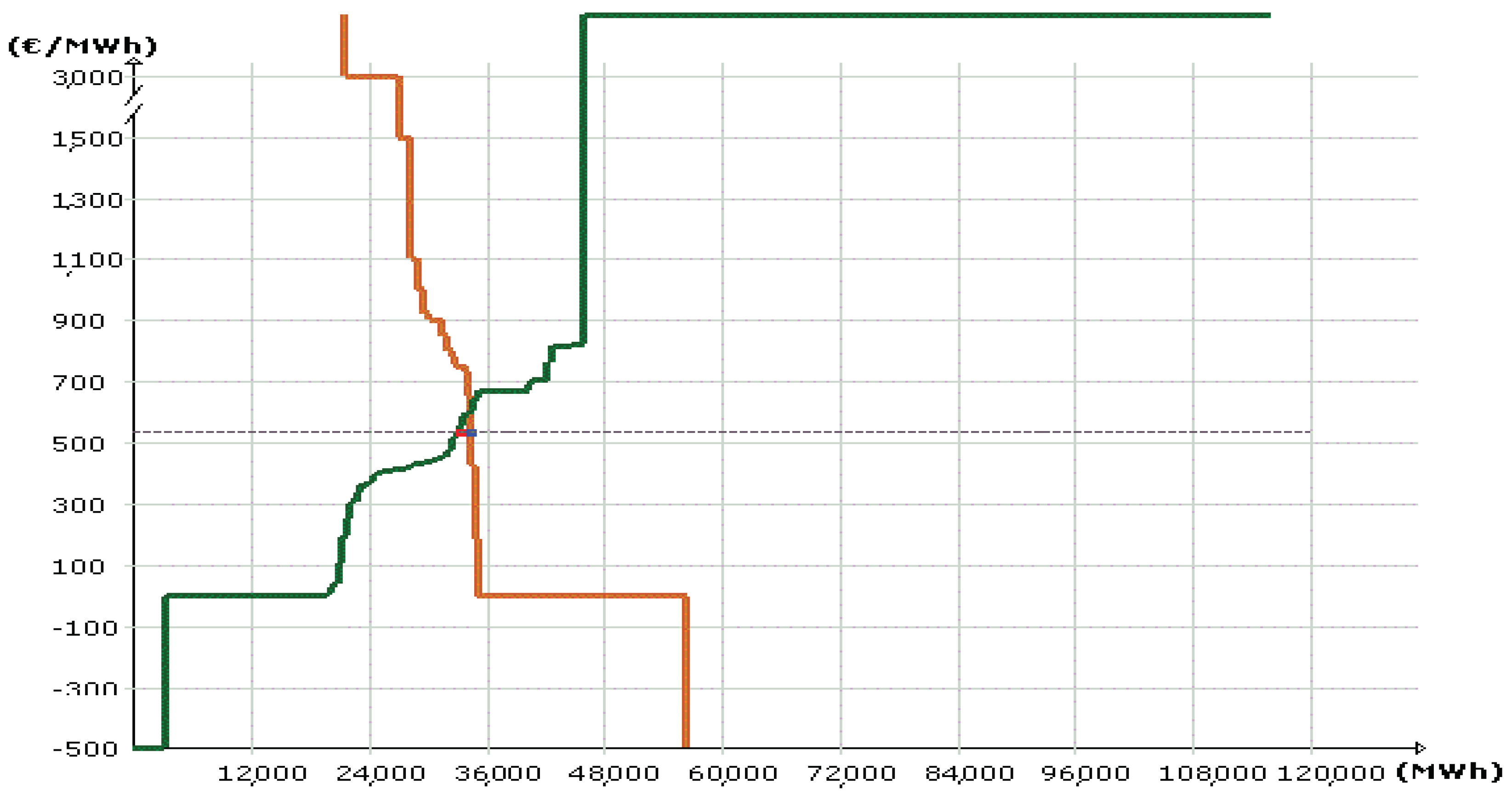
The DAM is an organized market for wholesale trading, where hourly blocks of electricity are negotiated until the day before the delivery is effectively executed. During the session, market participants submit supply offers/demand bids where they specify the volume and the minimum/maximum price at which they are willing to sell/purchase electricity. Therefore, offers/bids express a complete and well-defined optimal bidding strategy of the market participants. The DAM is organized according to an implicit double auction where supply offers and demand bids are accepted under the economic merit-order criterion and subjected to zonal transmission constraints; the algorithm constructs the aggregate supply curve by ranking the supply offers according to an increasing price order, while the aggregate demand curve is constructed by ranking the demand bids according to a decreasing price order. The intersection of the two curves gives the overall traded volume and the clearing price; only the supply offers/demand bids with price below/above the clearing price are admitted to inject/withdraw electricity. Therefore, the injection and withdrawal schedules are obtained as the sum of the accepted bids/offers. Then, the market operator clears the market with the system marginal price (SMP) paid to suppliers by zones, if there is a need for market splitting due to congestion, and PUN is paid by all buyers. Figure 2 shows an example of the market-clearing outcome occurring in the DAM.

Given the large availability of detailed historical data, market participants rely on forecasting methods based on econometric estimation and simulation models in order to optimize their bidding strategies. In this paper we exploit these micro-level data to construct the hourly empirical aggregate demands for 2020 and estimate the price elasticities using traditional regression models, where the aggregate demand is a linear function of bid prices and other structural variables. Thus, this paper presents a novel analysis in the literature, giving a more accurate picture of the electricity price responsiveness at exceptional times.

The paper is organized as follows: the data and the theoretical model which drive the empirical estimations are presented in Section 2; we present and discuss the results in Section 3; Section 4 is devoted to conclusions.

2. Material and Data

2.1. Model

The econometric approach used to estimate demand elasticity lies inside the neoclassical framework and is grounded in rational optimizing behavior theory. In the Italian wholesale electricity market, only eligible buyers can operate, and they are large buyers (energy-intensive industries, railways, telecom companies), industrial buyers and traders who can intermediate both small industrial and residential consumers. We assume that industrial consumers choose the amount of electricity input that minimizes their cost function given the technological constraints; similarly, residential customers choose the amount of electricity that minimizes their expenditure given a certain level of utility to be reached.

Since data refer to hourly bids, the duality approach gives the theoretical justification to legitimately switch from an agent’s preferences (optimization theory) to the Marshallian demand, where quantities are functions of prices and total expenditure. We assume that for both residential and industrial consumers it is possible to postulate the existence of a cost function for using electricity as a good “e” and a composite numerary good “x”:

In each hour of the day, all agents taking part in the DAM rationally behave minimizing a cost function C(p,Q), where p is the vector of prices of electricity and composite goods [p_e, p_x] and Q is the objective variable (production for industrial buyers and utility for residential ones). We assume that the cost function is continuous, increasing in Q, non-decreasing, linearly homogeneous and concave in prices. The cost minimization yields the system of equations called Hicksian demand functions, where the quantities demanded for each good i are expressed in terms of prices and the objective variable:

$$\frac{\partial C\left(p,q\right)}{\partial p_i}=h_i\left(p,Q\right)$$

(1)

Exploiting the homogeneity and separability properties of cost function and applying the Roy identity, the duality approach allows recovery of the Marshallian demand functions $y_e$ from the inverse function of the objective variable $Q=V\left(m,p\right)$, where m is the monetary expenditure. Replace V m with the expenditure function C(Q,p):

$$Q=V\left(m,p\right)=V\left(C\left(Q,p\right),p\right)$$

(2)

and differentiate V with respect to price and cost:

$$\frac{\raisebox{1ex}{$\partial V$}\!\left/ \!\raisebox{-1ex}{$\partial p$}\right.}{\raisebox{1ex}{$\partial V$}\!\left/ \!\raisebox{-1ex}{$\partial C$}\right.}=h_e\left(p,Q\right)=y_e\left(m, p\right)$$

(3)

We obtain, via the Roy identity, the Marshallian demand $y_e\left(m, p\right)$ that expresses the demand for electricity as a function of its own price $p_e$, the total expenditure $m$, and the price of the numerary good $p_x$. Equation (3) represents the hourly electricity demand of each participant in the DAM. It holds for each state of nature and for each hour and models short run behavior.

In order to recover the empirical demand functions, there is a need to specify the parametric functional form. We assume the Generalized Almost Ideal Demand System [30], that generalized the Almost Ideal demand system of [31] with the introduction of committed quantities:

$$y_{e,t}={\alpha }_t+{\beta }_t\ln \frac{p_{e,t}}{\overline{p}}+{\sum }_k{\gamma }_k{d}_{i,k}+{\upsilon }_{e,t}$$

(4)

The dependent variable $y_{e,t}$ is the hourly electricity demand of hour t, the explanatory variables are the committed quantity ${\alpha }_t$, the corresponding logarithm of price, $p_{e,t}$, adjusted by the monthly consumer index price $\overline{p}$, that meaningfully approximates $p_x$, and regressors $d_{i,k}$ that refer to a group of socioeconomic determinants and proxy the real total expenditure and the scale effect (i.e., the daily and zonal intercept dummies). ${\upsilon }_{e,t}$ is the error term distributed according to a normal $N\left(0, {\sigma }^2\right)$.

Given this linear form, price elasticity is computed as:

$${\epsilon }_t=\frac{\partial y_e}{\partial p_e}\frac{p_e}{y_e}=\frac{{\beta }_t}{y_e}$$

(5)

It is noteworthy that Equation (5) is directly derived from the consumer optimizing behavior and, thus, it includes both price and income effects. In this way, electricity price elasticity can be consistently estimated, considering both these effects.

2.2. Material

We used GME’s daily data gathered in monthly datasets starting from January to December 2020. Each monthly dataset accounts for about 2.1 million raw observations.

The preliminary investigation of the datasets was to provide an exhaustive analysis of the DAM highlighting its main features.

Table 1. Offer to Purchase (BID) and Sales (OFF): Monthly Total Quantity and Frequency.

	BID		OFF
	Quantity	Abs. Frequency	Quantity	Abs. Frequency
January	26.605	673,948	87.163	1,196,471
February	24.491	640,818	82.510	1,133,685
March	22.689	704,425	86.128	1,216,843
April	18.660	672,583	84.080	1,253,628
May	21.418	711,982	86.761	1,336,192
June	22.747	702,401	82.337	1,308,968
July	26.927	737,417	99.317	1,332,526
August	24.296	736,915	83.193	1,248,495
September	24.755	719,708	81.462	1,242,130
October	31.409	959,042	101.842	1,980,730
November	31.072	941,273	96.984	1,924,386
December	31.955	997,612	104.705	1,992,752
Mean	25.585	766,510	89.707	1,430,567

Note: Quantity is expressed in GWh.

shows, for each month of 2020, the total quantity of all offers to buy and sell electricity. The demand side shows levels of activity lower than the supply side. The total number of bids (Abs Frequency) is in fact lower, as well as the quantities of demanded electricity.

This result is more evident if we look at

Table 2. Offer to Purchase (BID) and Sales (OFF): Monthly Total Quantity and Frequency of Accepted and Rejected Offers.

	BID				OFF
	Accepted		Rejected		Accepted		Rejected
	Quantity	Abs. Frequency	Quantity	Abs. Frequency	Quantity	Abs. Frequency	Quantity	Abs. Frequency
January	25.834	600,244	0.771	73,704	24.249	967,298	62.915	229,173
February	23.811	569,884	0.680	70,934	21.833	897,546	60.677	236,139
Marcgh	22.037	629,286	0.653	75,139	20.087	915,668	66.041	301,175
April	18.167	598,999	0.493	73,584	17.920	881,267	66.160	372,361
May	21.029	627,903	0.389	84,079	20.339	940,539	66.423	395,653
June	22.193	613,164	0.554	89,237	22.135	967,115	60.202	341,853
July	26.281	642,460	0.645	94,957	36.989	1,009,141	62.328	323,385
August	23.725	659,006	0.571	77,909	23.072	943,095	60.120	305,400
September	23.938	629,570	0.818	90,138	23.473	937,980	57.989	304,150
October	23.411	650,620	7.998	308,422	21.490	944,048	80.352	1,036,682
November	23.361	640,803	7.859	300,470	21.429	917,008	75.554	1,007,378
December	24.096	672,216	7.859	325,396	22.662	944,091	82.043	1,048,661
Mean	23.157	627,846	2.441	138,664	22.973	938,733	66.734	491,834

Note: Quantity is expressed in GWh.

where we split the offers to purchase and sale of electricity between accepted and rejected offers.

The monthly sums of all accepted bids and offers, respectively, the first and fifth columns, are essentially the same and amount to an average of 23 GWh; small differences will be adjusted in the four intra-day markets. If we look at the rejected offers, we notice that, on the demand side, the rejected offers to purchase account for a minimum part of the overall monthly demand; they represent only 2.441 GWh, on average, and their absolute frequency is about 22% of the total number of accepted bids. Looking instead at the supply side, we see that the rejected offers to sell are far larger than those accepted; they represent on average 66.734 GWh, roughly three times the accepted quantity, and their absolute frequency is about 52% of the total number of accepted offers. This highlights a degree of competition on the supply side higher than that on the demand side. We retained only the observations referring to the demand side (BID); these observations account for about 35–40% of the whole monthly datasets.

There are two relevant features in the DAM. First, there are heterogeneous consumers whose bids do not specify the price at which to buy electricity; these bids refer to consumers who show ex ante a perfect inelastic behavior, as they are (in principle) willing to pay any price that would result from the market-clearing procedure. The GME assigns to these bids a fictitious price equal to the supply price cap that is equal to 3000 euro/MWh. (The DAM assigns a default price limit to these bids, set equal to the maximum price cap imposed on suppliers by the Regulatory Authority. The default price assigned to these bids has increased in time from a level of 200 euro/MWh in 2004 to 3000 euro/MWh since 2009).

Table 3. Offer to Purchase (BID): Monthly Relative Frequency and Total Quantity of Inelastic and Elastic Bids.

	Inelastic Bid		Elastic Bid
	Relative Frequency	Quantity	Relative Frequency	Quantity
January	76.751	24.052	23.249	1.782
February	76.000	22.375	24.000	1.436
March	75.207	20.783	24.793	1.254
April	75.652	17.092	24.348	1.075
May	74.391	19.773	25.609	1.256
June	73.848	20.878	26.152	1.315
July	73.931	24.890	26.069	1.391
August	72.302	22.354	27.698	1.371
September	73.609	22.697	26.391	1.241
October	73.451	22.276	26.549	1.136
November	73.320	21.924	26.680	1.437
December	73.925	22.641	26.075	1.454
Mean	74.366	21.811	25.634	1.346

Note: Quantity is expressed in GWh.

shows that these bids represent most of the accepted bids (on average the 74% of the total number of accepted bids) and most of the electricity monthly purchased, about 21.736 GWh, refers to buyers characterized by rigid demand. Other consumers specify instead in their bids both quantity and price and, in turn, they should be considered elastic consumers.

Second, agents who submit demand bids are not necessarily the final users of electricity. Single Buyers and traders are intermediary agents that demand electricity on behalf of final customers and their behaviors should be processed into the model. The contractual nature of the trader–customer relationship suggests that this can be treated within the perspective of the principal–agent relationship, where consumer is the principal and trader is the agent. Under these conditions, we assume that traders’ utility is aligned with that of the final customer (see [32,33]).

Table 4. Offer to Purchase (BID): Monthly Total Quantity and Absolute Frequency of Accepted Bids, Monthly Share and Relative Frequency Single Buyer and Bilateral Contracts.

	Purchases		Single Buyer		Bilateral Contracts
	Quantity	Abs. Frequency	Share	Frequency %	Share	Frequency %
January	25.83	600,244	16.77	0.74	39.38	34.78
February	23.81	569,884	16.33	0.73	40.88	34.21
March	22.04	629,286	17.24	0.71	42.71	33.61
April	18.17	598,999	18.14	0.72	45.57	34.41
May	21.03	627,903	15.54	0.71	43.09	33.08
June	22.19	613,164	14.77	0.70	42.78	32.72
July	26.28	642,460	15.17	0.69	39.41	31.81
August	23.72	659,006	16.69	0.68	39.94	31.80
September	23.94	629,570	13.07	0.69	42.15	33.44
October	23.41	650,620	13.17	0.69	41.85	32.91
November	23.36	640,803	14.43	0.67	40.71	32.43
December	24.10	672,216	15.80	0.66	38.85	31.84
Mean	23.16	627,846	15.59	0.70	41.44	33.09

Note: Quantity is expressed in GWh.

shows, for each month of 2020, the overall quantity of accepted bids, that is essentially the electricity purchased during each month, and its absolute frequency. On average the monthly purchases account for 23 GWh, but if we look at the months of March, April and May, the period of the heavy lockdown, the levels of electricity purchased are the lowest.

The sum of accepted purchase offers is on average equal to 23.16 GWh; 15.59% comes from the Italian Single Buyer, while 41.44% is from bilateral contracts. (The Italian Power Exchange is a voluntary market: purchase and sale contracts may also be concluded off the exchange platform, i.e., bilaterally or over the counter (OTC)) For these purchase offers, the price is not known, but the quantity must instead be explicit in order to better schedule the withdrawal and injection programs into the transmission grid. Bids referring to bilateral contracts are in fact always accepted and, thus, participate in constructing the rigid segment of the aggregate demand. Bilateral bids derive from bargaining external to the DAM, and, as a consequence, for these bids it is not possible to observe the price responsiveness. Therefore, we consider these bids as if they were inelastic, forming the rigid part of the aggregate demand curve.

It is assumed that electricity demand profiles substantially differ within the day. The hours between 9 a.m. and 9 p.m. (though as the group of peak hours) are assumed as being characterized by the prevalence of business activities and high levels of load, with the hours between 10 p.m. and 8 a.m. (defined as the group of off-peak hours) being characterized by the prevalence of domestic use of electricity.

Table 5. Equilibrium Prices and Quantities in the DAM. Monthly Average.

	Price		Quantity
	Peak	Off-Peak	Peak	Off-Peak
January	52.104	41.989	40.098	29.323
February	42.776	35.196	38.854	29.297
March	34.835	28.627	33.096	25.740
April	24.472	25.199	27.753	23.016
May	21.697	21.896	31.242	25.423
June	28.331	27.627	34.672	27.422
July	39.691	36.014	39.272	30.967
August	41.562	38.850	35.311	28.426
September	53.100	43.720	37.262	28.992
October	47.367	39.099	35.246	26.983
November	54.531	41.913	37.075	27.318
December	62.864	43.604	37.324	27.359
Mean	41.944	35.311	35,601	27,522

Note: Quantities are expressed in GWh. The resulting Equilibrium quantities account for the adjustments in the Inframarginal Markets.

reports the monthly summary statistics for equilibrium market prices and quantities and confirms this assumption.

The average quantity purchased in the off-peak hours is, on average, 25% lower than the quantity recorded in the peak hours. Differences can be noticed also in the PUN: during the peak hours, the equilibrium prices are, on average, roughly equal to 42 euro/MWh, 7 euros higher than the average price recorded during off-peak hours.

Alongside the hourly variation, 2020 recorded strong differences among months, due to lockdown.

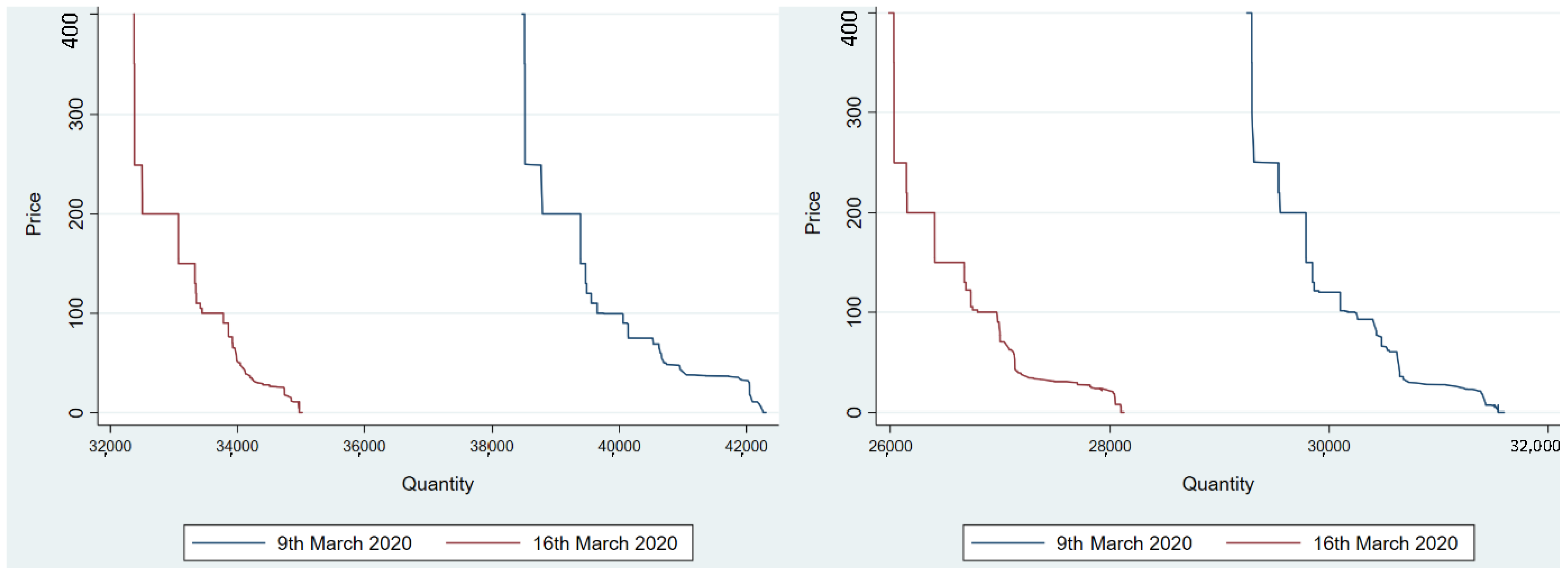
In Italy, the lockdown policy was announced for the northern part of the country on the 8 March and was extended to the whole nation on the 10 March. The restriction policy was clearly reflected in the shrink in the electricity demand. This is particularly evident in the first graph on the left of Figure 3 that depicts the empirical aggregate demands referring to two different days of March 2020. The blue curve defines the electricity demand concerning the 12 a.m. of Monday 9 March, one day before the lockdown was announced. The red curve defines instead the aggregate electricity demand concerning the 12 a.m. of Monday 16 March, when the lockdown had just been started. If we look at the horizontal intercept, for the same peak-hour of a work day, the electricity demand underwent a shift of roughly seven thousand MWh, passing from forty-two thousand, three hundred MWh to thirty-five thousand MWh. The peak daily electricity consumption dropped by nearly 20% in the third week in March when full lockdown was applied. The same shift was recorded in the electricity demand of the off-peak hours. The graph on the right of Figure 3 shows the two different positions of the aggregate demand referring to 0 a.m. of the 9 and 16 March. Also in this case, the horizontal intercept of the aggregate demand moved to the left from 31.6 to 28.2 thousand MWh.

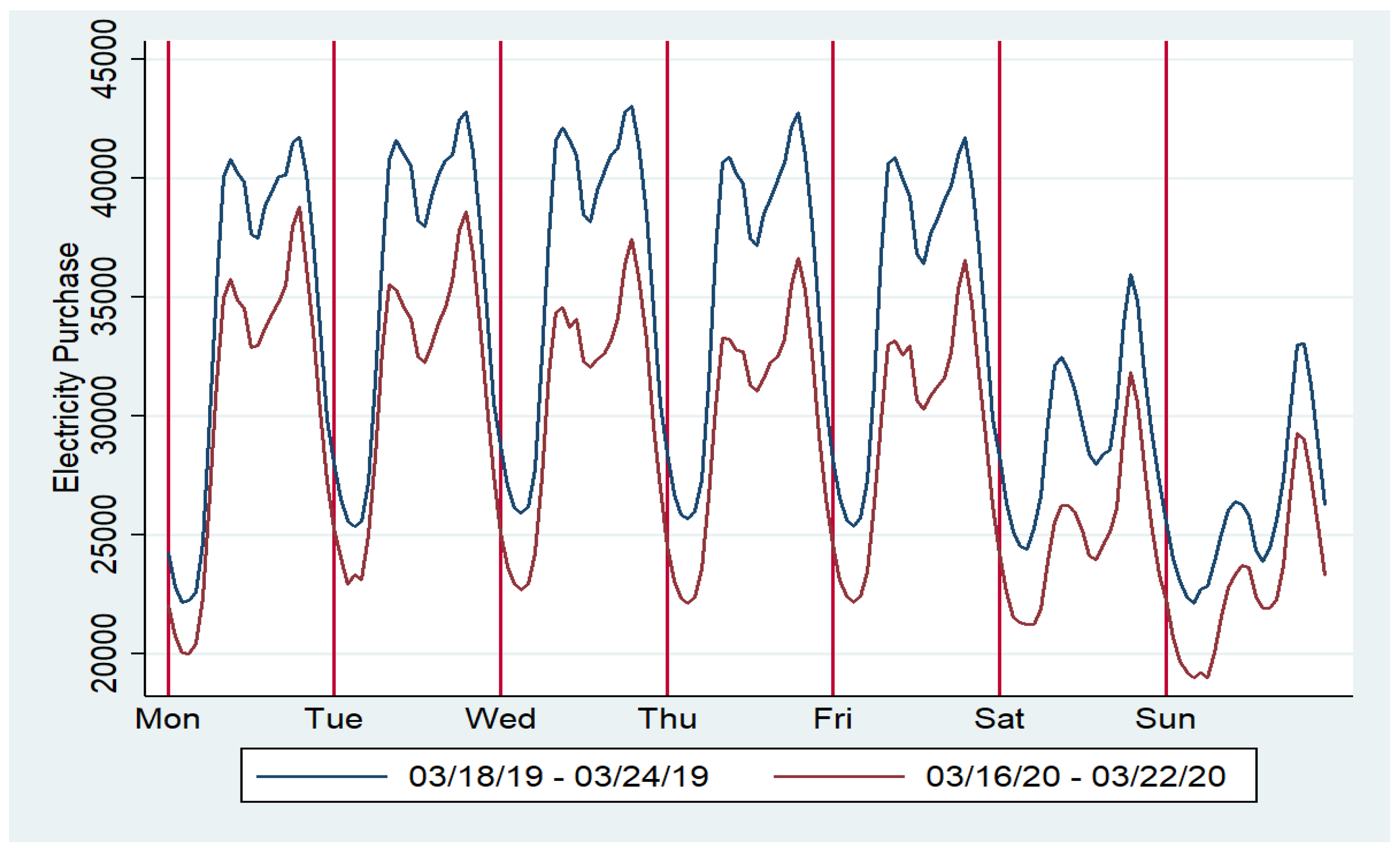
In Figure 4, we compare the national load profiles during the third week of March 2019 (18 March–24 March) with the load profiles recorded in the third week of March 2020 (16 March–22 March), when lockdown had just begun. Also, this figure shows that the weekly load profiles translated down by nearly 20%.

We are going to analyze the annual variation in equilibrium prices and quantities between 2019 and 2020.

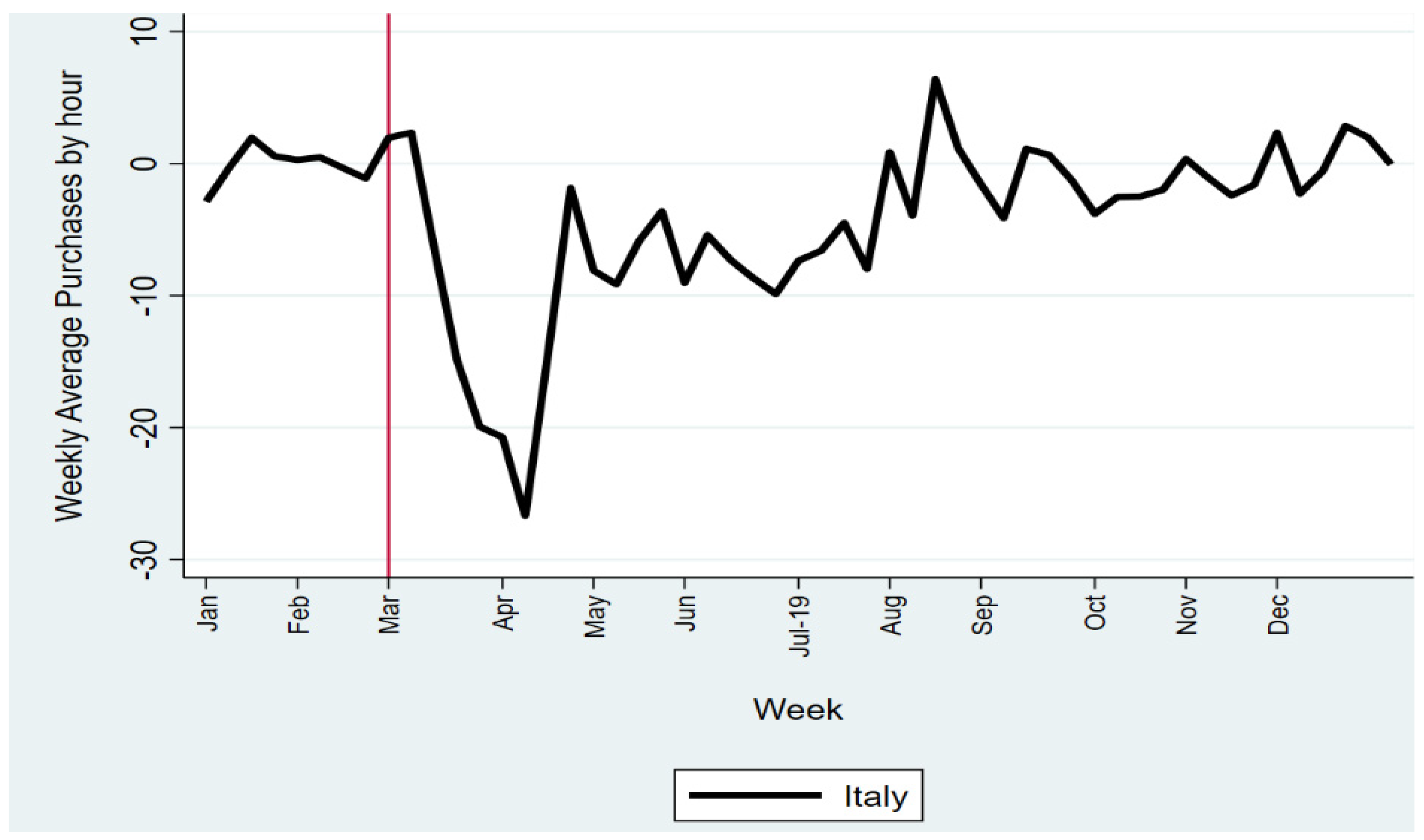
Figure 5 shows the weekly average of the relative annual variation of market prices. The bold black line identifies the pattern of the variation of the PUN; the colored lines identify instead the variations of the zonal prices. It is noteworthy to mention that when lockdown measures came into effect, all prices started immediately falling; only Sicily shows a lag in the plunge of the weekly average price. Prices started recovering from June 2020, when all lockdown measures were suppressed. At the end of September, a new upward trend was recorded and, in October, the annual price variation turned positive. In particular, Sicily’s average price variation recorded the spikiest pattern, starting from September, when the pandemic crisis began to rekindle.

Looking at total purchases, at the beginning of March the weekly average of the annual variation started falling, reaching the lowest level at the beginning of April (Figure 6).

3. Empirical Results and Discussion

We constructed the aggregate demand curves for each hour of the day. Bids representing inelastic behavior were lumped into one aggregated observation, defining the vertical intercept of the aggregate demand.

At the end of the procedure, the average sample size of the monthly datasets was 257,570, ranging from 205,935 observations, recorded in February, to 342,273 observations, recorded in December.

Then, the elasticity of each hourly demand curve is estimated using a linear regression model. Each linear regression accounts for about 354 observations. Note that bids are expressed by different operators in every hour, so the regression errors are not autocorrelated.

The summary statistics of the elasticity estimates aggregated by hour are reported in

Table 6. Summary Statistics of the Hourly Elasticity Estimates.

Hour		Max	Mean	Min
1	$\mathsf{\epsilon }$	−0.2342	−0.0281	−0.0037
	$\mathrm{Var}\left(\mathsf{\epsilon }\right)$	0.0000	0.0001	0.0009
2	$\mathsf{\epsilon }$	−0.2339	−0.0276	−0.0036
	$\mathrm{Var}\left(\mathsf{\epsilon }\right)$	0.0000	0.0001	0.0009
3	$\mathsf{\epsilon }$	−0.2319	−0.0269	−0.0036
	$\mathrm{Var}\left(\mathsf{\epsilon }\right)$	0.0000	0.0001	0.0009
4	$\mathsf{\epsilon }$	−0.2387	−0.0271	−0.0036
	$\mathrm{Var}\left(\mathsf{\epsilon }\right)$	0.0000	0.0001	0.0009
5	$\mathsf{\epsilon }$	−0.2193	−0.0267	−0.0034
	$\mathrm{Var}\left(\mathsf{\epsilon }\right)$	0.0000	0.0001	0.0008
6	$\mathsf{\epsilon }$	−0.2220	−0.0262	−0.0035
	$\mathrm{Var}\left(\mathsf{\epsilon }\right)$	0.0000	0.0000	0.0008
7	$\mathsf{\epsilon }$	−0.2172	−0.0272	−0.0041
	$\mathrm{Var}\left(\mathsf{\epsilon }\right)$	0.0000	0.0001	0.0007
8	$\mathsf{\epsilon }$	−0.2218	−0.0250	−0.0047
	$\mathrm{Var}\left(\mathsf{\epsilon }\right)$	0.0000	0.0000	0.0008
9	$\mathsf{\epsilon }$	−0.2215	−0.0247	−0.0039
	$\mathrm{Var}\left(\mathsf{\epsilon }\right)$	0.0000	0.0001	0.0008
10	$\mathsf{\epsilon }$	−0.1944	−0.0242	−0.0039
	$\mathrm{Var}\left(\mathsf{\epsilon }\right)$	0.0000	0.0000	0.0008
11	$\mathsf{\epsilon }$	−0.1856	−0.0249	−0.0039
	$\mathrm{Var}\left(\mathsf{\epsilon }\right)$	0.0000	0.0001	0.0006
12	$\mathsf{\epsilon }$	−0.1320	−0.0249	−0.0040
	$\mathrm{Var}\left(\mathsf{\epsilon }\right)$	0.0000	0.0001	0.0005
13	$\mathsf{\epsilon }$	−0.2107	−0.0250	−0.0037
	$\mathrm{Var}\left(\mathsf{\epsilon }\right)$	0.0000	0.0000	0.0007
14	$\mathsf{\epsilon }$	−0.2129	−0.0246	−0.0036
	$\mathrm{Var}\left(\mathsf{\epsilon }\right)$	0.0000	0.0000	0.0007
15	$\mathsf{\epsilon }$	−0.2025	−0.0244	−0.0039
	$\mathrm{Var}\left(\mathsf{\epsilon }\right)$	0.0000	0.0000	0.0007
16	$\mathsf{\epsilon }$	−0.2099	−0.0253	−0.0039
	$\mathrm{Var}\left(\mathsf{\epsilon }\right)$	0.0000	0.0001	0.0007
17	$\mathsf{\epsilon }$	−0.1999	−0.0247	−0.0041
	$\mathrm{Var}\left(\mathsf{\epsilon }\right)$	0.0000	0.0001	0.0007
18	$\mathsf{\epsilon }$	−0.2127	−0.0261	−0.0041
	$\mathrm{Var}\left(\mathsf{\epsilon }\right)$	0.0000	0.0001	0.0007
19	$\mathsf{\epsilon }$	−0.2426	−0.0267	−0.0043
	$\mathrm{Var}\left(\mathsf{\epsilon }\right)$	0.0000	0.0001	0.0010
20	$\mathsf{\epsilon }$	−0.2736	−0.0259	−0.0042
	$\mathrm{Var}\left(\mathsf{\epsilon }\right)$	0.0000	0.0001	0.0014
21	$\mathsf{\epsilon }$	−0.2298	−0.0252	−0.0044
	$\mathrm{Var}\left(\mathsf{\epsilon }\right)$	0.0000	0.0001	0.0010
22	$\mathsf{\epsilon }$	−0.2426	−0.0261	−0.0042
	$\mathrm{Var}\left(\mathsf{\epsilon }\right)$	0.0000	0.0001	0.0010
23	$\mathsf{\epsilon }$	−0.2252	−0.0273	−0.0034
	$\mathrm{Var}\left(\mathsf{\epsilon }\right)$	0.0000	0.0001	0.0008
24	$\mathsf{\epsilon }$	−0.2251	−0.0278	0.0000
	$\mathrm{Var}\left(\mathsf{\epsilon }\right)$	0.0000	0.0001	0.0008
Mean	$\mathsf{\epsilon }$	−0.2736	−0.0259	0.0000
	$\mathrm{Var}\left(\mathsf{\epsilon }\right)$	0.0000	0.0001	0.0014

Note: ε stands for the elasticities estimate, Var(ε) denotes the variance of variance.

. For each hour, the first row concerns the averages (minimum, mean and maximum) of the elasticity estimates, the second row refers instead to the variances. On average, the hourly elasticity demand is roughly −0.0259 (In the following, we refer to values of elasticities in absolute terms, given that demand elasticities are typically negative. So, we refer to "higher elasticity" when the absolute value is higher even if the algebraic number is more negative and therefore "lower”), ranging between −0.27, recorded at 8 p.m., and 0 recorded at 0 a.m. The lowest (absolute) level of elasticity is recorded at 0 a.m., showing that demand is inelastic when it refers to hours characterized by less flexible industrial uses; that is, when electricity is an input of productions that cannot be stopped. Coefficient estimates are all significant; if we look at the summary statistics of the variance, we see that values are really low, ranging between 0 and −0.0014.

Looking at the column Mean, containing the averages of the elasticity estimates, peak hours record lower levels of elasticity. This finding is shown in

Table 7. Summary Statistics of the Hourly Elasticity Estimates, Aggregated by Peak and Off-peak Hours.

Hour		Max	Mean	Min
Peak	$\mathsf{\epsilon }$	−0.2736	−0.0251	−0.0036
	$\mathrm{Var}\left(\mathsf{\epsilon }\right)$	0.0000	0.0001	0.0014
Off-peak	$\mathsf{\epsilon }$	−0.2426	−0.0269	0.0000
	$\mathrm{Var}\left(\mathsf{\epsilon }\right)$	0.0000	0.0001	0.0010

Note: ε stands for the elasticities estimate, Var(ε) denotes the variance of variance.

; the average elasticity among hours between 9 a.m. and 9 p.m. is −0.0251 against an average of −0.0269 recorded for the hours between 10 p.m. and 8 a.m.

If we aggregate elasticities according to four different periods characterizing the different degrees of stringency of the lockdown measures we see that values show strong differences.

The four periods are listed as follows: (i) the pre-lockdown period (1 January–9 March) where all economic activity ran as usual; (ii) the complete lockdown period (10 March–3 June) with the total shutdown of human movement, except for a few essential activities, such as visits to food shops and pharmacies; (iii) the post-lockdown period (3 June–30 September), where all economic activity gradually resumed with the re-opening of restaurants, salons, shopping centers, while maintaining social distance and wearing face masks; (iv) the last period (1 October–31 December), when contagion began to spread again and the health emergency resumed, with new lockdown measures imposed by the central government. In the Appendix A we show different levels of aggregation (by month) of the elasticity estimates.

Table 8. Summary Statistics of the Hourly Elasticity Estimates, Peak and Off-peak Hours, aggregated by different periods of the year.

	Peak			Off-Peak
	Max	Mean	Min	Max	Mean	Min
1 January–9 March	−0.0188	−0.0097	−0.0036	−0.0181	−0.0106	−0.0043
10 March–2 June	−0.0141	−0.0072	−0.0039	−0.0142	−0.0070	0.0000
3 June–30 September	−0.0387	−0.0096	−0.0039	−0.0344	−0.0092	−0.0036
1 October–31 December	−0.2736	−0.0728	−0.0081	−0.2426	−0.0798	−0.0117
Mean	−0.2736	−0.0251	−0.0036	−0.2426	−0.0269	0.0000

shows the summary statistics (the mean, minimum and the maximum) of the hourly elasticity estimates aggregated by the four different periods.

During the lockdown period demand elasticity reduced, underlining how energy demand was mainly expressed by essential economic activities characterized by low price responsiveness. In the mentioned period, the average elasticity moved from −0.0097 to −0.0072 in the peak hours, and, similarly, from −0.0106 to −0.0070 in the off-peak hours. When economic activities gradually resumed (the summer period between 3 June and 30 September), elasticity recorded a light recovery, reaching an average value slightly below the threshold of 1% (−0.0096 and −0.0092 for the peak and off-peak hours, respectively). The most important change was recorded in the last period, when the average price responsiveness of energy demand increased by roughly eight times, reaching values equal to −0.0728 and −0.0798 in the peak and off-peak hours, respectively. Even the range between the minimum and the maximum enlarged, highlighting an increase in the volatility of price responsiveness. The maximum values were −0.081 and −0.0117 while the minimum were −0.2736 and −0.2426, in the peak and off-peak hours, respectively. These figures seem to suggest that as lockdown measures were restored due to the new spread of contagion, economic activities were able to structure their demand, making themselves flexible to price changes in a way that, in the first period of the health emergency, they had not been able to do.

If we disaggregate elasticities according to the day of the week we do not see large differences among days.

Table 9. Mean of the Hourly Elasticity Estimates, Peak and Off-peak Hours, aggregated by different periods of the year and Days of the Week.

		Monday	Tuesday	Wednesday	Thursday	Friday	Satarday	Sunday
1 January–9 March	Peak	−0.0094	−0.0097	−0.0091	−0.0097	−0.0102	−0.0099	−0.0096
	Off-Peak	−0.0096	−0.0111	−0.0100	−0.0108	−0.0115	−0.0110	−0.0102
10 March–2 June	Peak	−0.0067	−0.0076	−0.0075	−0.0077	−0.0071	−0.0073	−0.0067
	Off-Peak	−0.0063	−0.0073	−0.0078	−0.0073	−0.0068	−0.0069	−0.0064
3 June–30 September	Peak	−0.0099	−0.0106	−0.0092	−0.0092	−0.0089	−0.0097	−0.0095
	Off-Peak	−0.0096	−0.0103	−0.0092	−0.0090	−0.0087	−0.0091	−0.0087
1 October–31 December	Peak	−0.0926	−0.0666	−0.0697	−0.0599	−0.0590	−0.0680	−0.0950
	Off-Peak	−0.0984	−0.0745	−0.0797	−0.0681	−0.0672	−0.0728	−0.0991
Average	Peak	−0.0296	−0.0236	−0.0239	−0.0216	−0.0213	−0.0238	−0.0302
	Off-Peak	−0.0310	−0.0258	−0.0267	−0.0238	−0.0236	−0.0250	−0.0311

shows the averages by days of the week aggregated by peak and off-peak hours. Differences among different periods still emerge. The last period is the only one recording elasticity higher than average for all the days of the week; the other periods show instead elasticities lower than average. If we consider the sample represented by the daily elasticities (grouped by peak and off-peak hour) we can say that its distribution is right-skewed, with few high values. The right tail of the sample distribution is then represented by the values recorded in the last period. In the first three periods, the highest average elasticities were recorded during work days. In the peak hour group, Friday, Thursday and Monday recorded the highest elasticities for the first, second and third periods, respectively. In the off-peak group, the highest average elasticities were instead recorded on Friday, Wednesday and Tuesday. However, within these periods, differences between the different days of the week are small. The situation changes when we look at the last period, where the highest average values of the estimates were recorded during Sunday within both the groups of peak and off-peak hours (−0.0950 and −0.0991, respectively), confirming the traditional pattern that during public holidays electricity demand is less stiff. However, similar figures were recorded for a working day such as Monday.

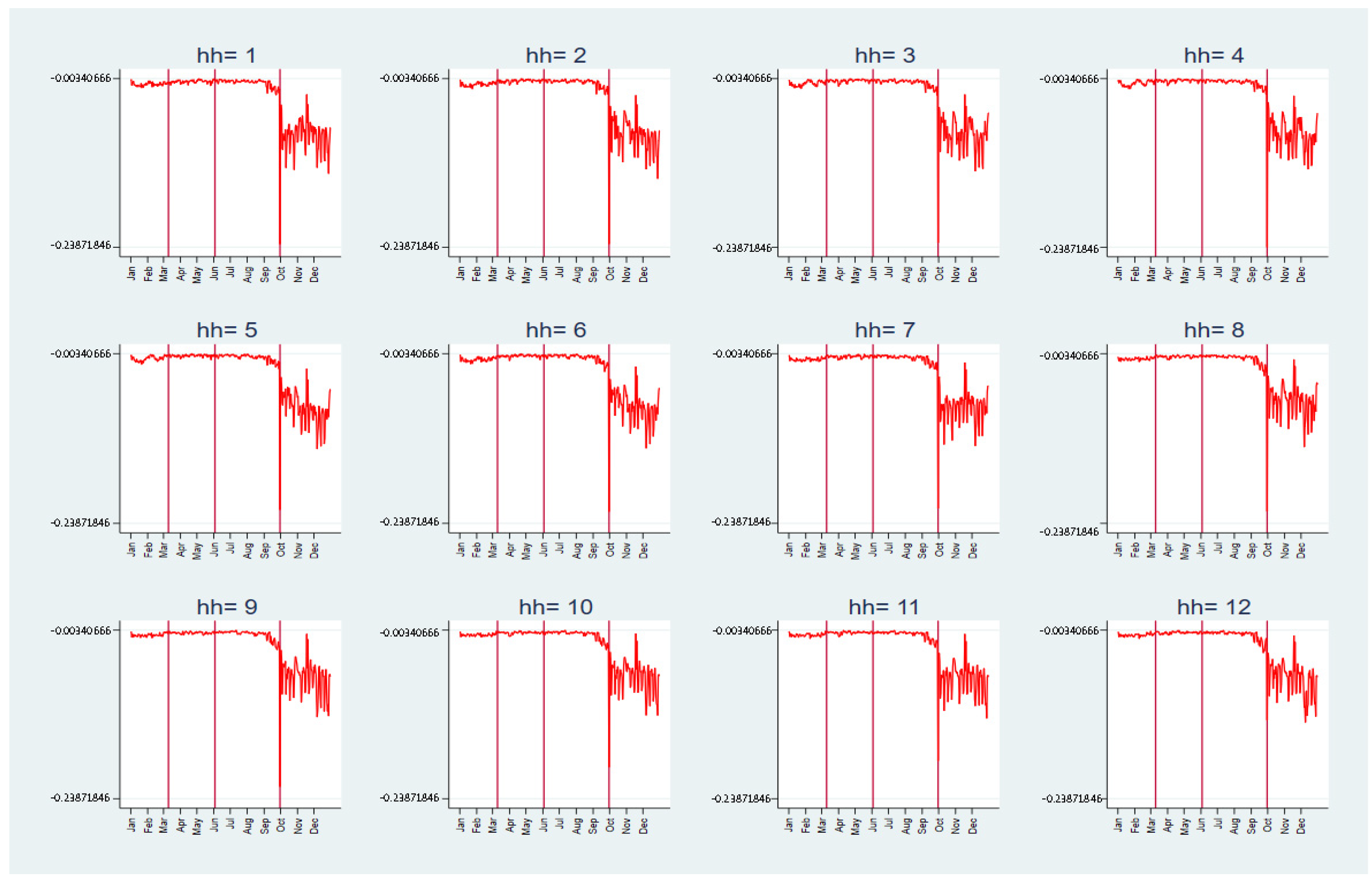
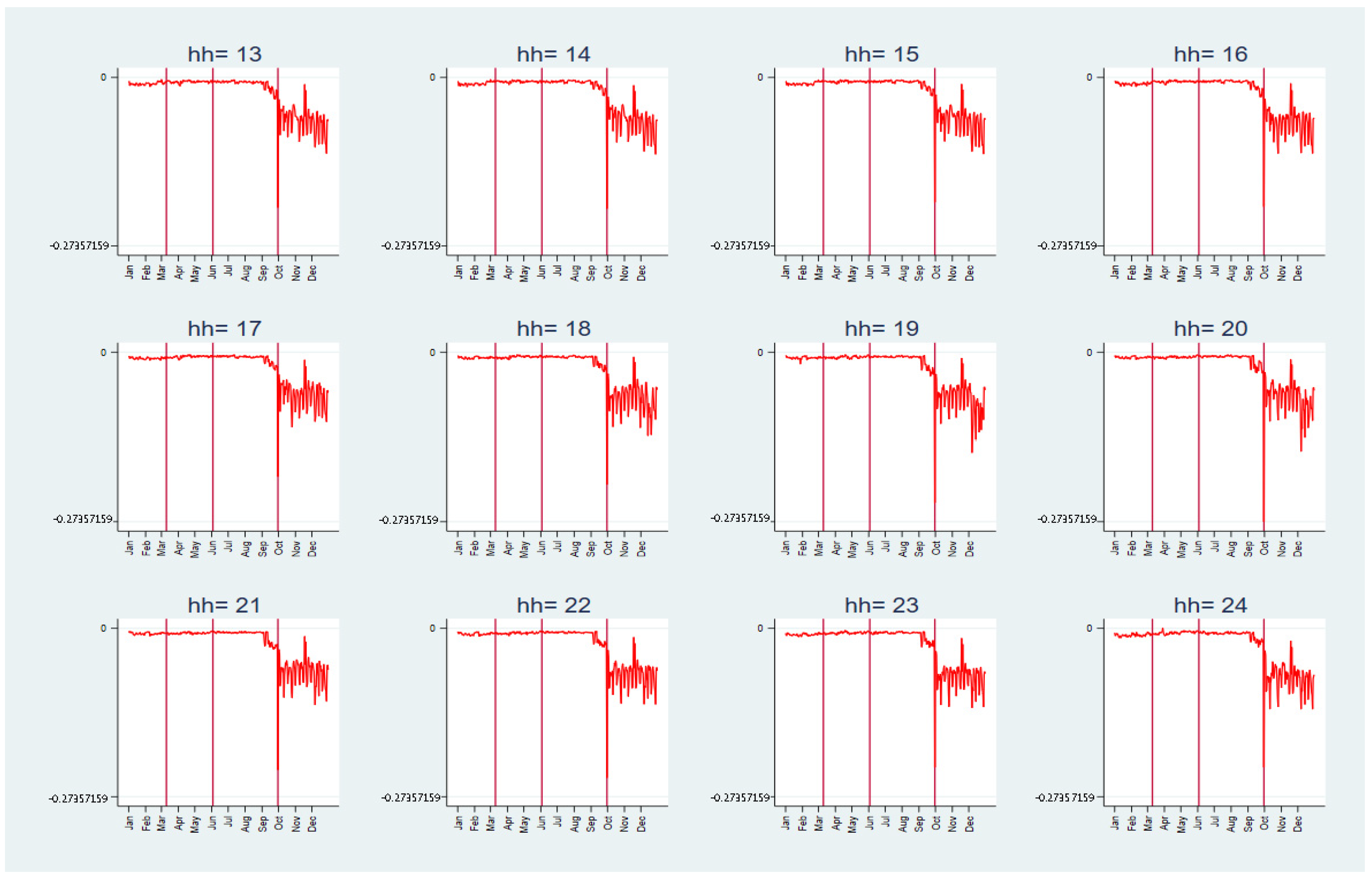
These kinds of aggregation do not allow for in-depth analysis of the daily changes in price responsiveness. The dynamics of hourly elasticities over 2020 are shown in Figure 7 and Figure 8. In each graph, we select the elasticity estimates referring to a specific hour and we plot their evolutions over time. From the graphs, a structural break emerges at the end of September, more precisely on 30 September. On this day, all elasticities show a dramatic change in their dynamic. Until September, their patterns were stable with low variability, then their dynamics recoded numerous downward spikes, and the range of variation significantly enlarged.

This result may be linked to the shocks and changes in electricity supply concerning energy source prices and power generation technologies. If we look at the marginal technologies fixing the price over the zonal markets (

Table 10. Average Frequency of Marginal Technology According to the Different Periods of 2020.

NORD	1 January–9 March	10 March–2 June	3 June–30 September	1 October–31 December
Coal	7.67	0.74	1.82	4.16
RES	17.87	22.61	16.67	15.90
Gas	55.07	52.72	36.10	42.36
Oil	0.48	0.39	0.56	1.21
Other	18.90	23.54	44.85	36.36
CNOR	1 January–9 March	10 March–2 June	3 June–30 September	1 October–31 December
Coal	8.82	1.96	7.21	5.06
RES	17.03	21.09	14.67	15.23
Gas	55.74	56.79	40.62	43.13
Oil	0.42	0.34	1.33	2.19
Other	18.00	19.81	36.17	34.39
CSUD	1 January–9 March	10 March–2 June	3 June–30 September	1 October–31 December
Coal	14.86	6.47	8.82	11.06
RES	15.94	20.40	13.83	14.78
Gas	52.90	54.68	41.70	46.22
Oil	0.72	0.25	1.40	2.73
Other	15.58	18.20	34.24	25.21
SUD	1 January–9 March	10 March–2 June	3 June–30 September	1 October–31 December
Coal	14.25	6.42	8.16	10.39
RES	16.73	21.33	13.66	14.87
Gas	53.62	55.22	44.71	49.04
Oil	0.72	0.25	1.54	3.18
Other	14.67	16.77	31.93	22.53
SICI	1 January–9 March	10 March–2 June	3 June–30 September	1 October–31 December
Coal	8.76	5.35	2.66	4.03
RES	14.19	20.70	7.49	6.76
Gas	63.65	57.04	74.16	74.38
Oil	0.06	0.54	1.68	1.34
Other	13.35	16.38	14.01	13.48
SARD	1 January–9 March	10 March–2 June	3 June–30 September	1 October–31 December
Coal	14.86	5.84	9.07	11.60
RES	15.94	23.20	15.90	14.73
Gas	52.90	53.21	40.20	45.95
Oil	0.72	0.25	1.37	2.69
Other	15.58	17.51	33.47	25.03
ITALY	1 January–9 March	10 March–2 June	3 June–30 September	1 October–31 December
Coal	11.53	4.46	6.29	7.72
FER	16.28	21.55	13.70	13.71
Gas	55.65	54.95	46.25	50.18
Oil	0.52	0.34	1.31	2.22
Other	16.01	18.70	32.45	26.17

Source: Our elaboration of GME Dataset.

), their frequencies completely change over the four periods.

The coal plants, which in the pre-COVID period (1 January–9 March) were the closing technology 11% of the time, during the lockdown period set the zonal price only 4% of the time. In the last period, and in all zonal markets, coal plants returned to being the closing technology 7.72 % of the time, even if they did not reach the levels recorded at the beginning of the year.

Renewable energy sources (RES) recorded instead an increase during the lockdown period: given the lower demand, they increased their opportunity to meet overall requirements and set marginal prices. Indeed, during the pre-lockdown period, they were the closing technology 16% of the time (on average), while during the heavy lockdown period this percentage increased to 21%. After this period, the percentage stabilized at the pre-lockdown values (We have to mention that RES technology, along with traditional solar, wind, and geothermal technologies, includes also hydro technology: pumped storage hydro power plants, run of the river hydro power plants, and reservoir hydro power plants. Both groups of technologies increased their frequencies of being a closing technology during the heavy lockdown period. Moreover, at the end of this period, all kinds of technology returned to traditional frequencies of being closing technology).

Gas technologies, which include combined cycle gas turbines, natural gas conventional thermal plants and gas turbines, in the pre-COVID period were the closing technologies about 55% of the time (on average) given their traditional function to cater to demand peaks. This percentage did not change during the lockdown period, and this is an unexpected result, since the consistent shrink in electricity demand suggests a decrease in the employment of peak-load plants. Moreover, if we look at the hours where gas technologies were the marginal technologies, we see that they essentially refer to the night. In the last two periods, the frequency of gas-closing technologies decreased, probably replaced by the RES technologies.

Oil-based plants recorded the most important increase; the average frequency with which they turned out to be the marginal technology went, on average, from 0.5% in the pre-lockdown period to 2% in the last period. The category “Other” recorded the greatest increase. Within this group, we included other technologies different from those mentioned before: uncertain technologies, market coupling technologies, and foreign virtual zones technologies.

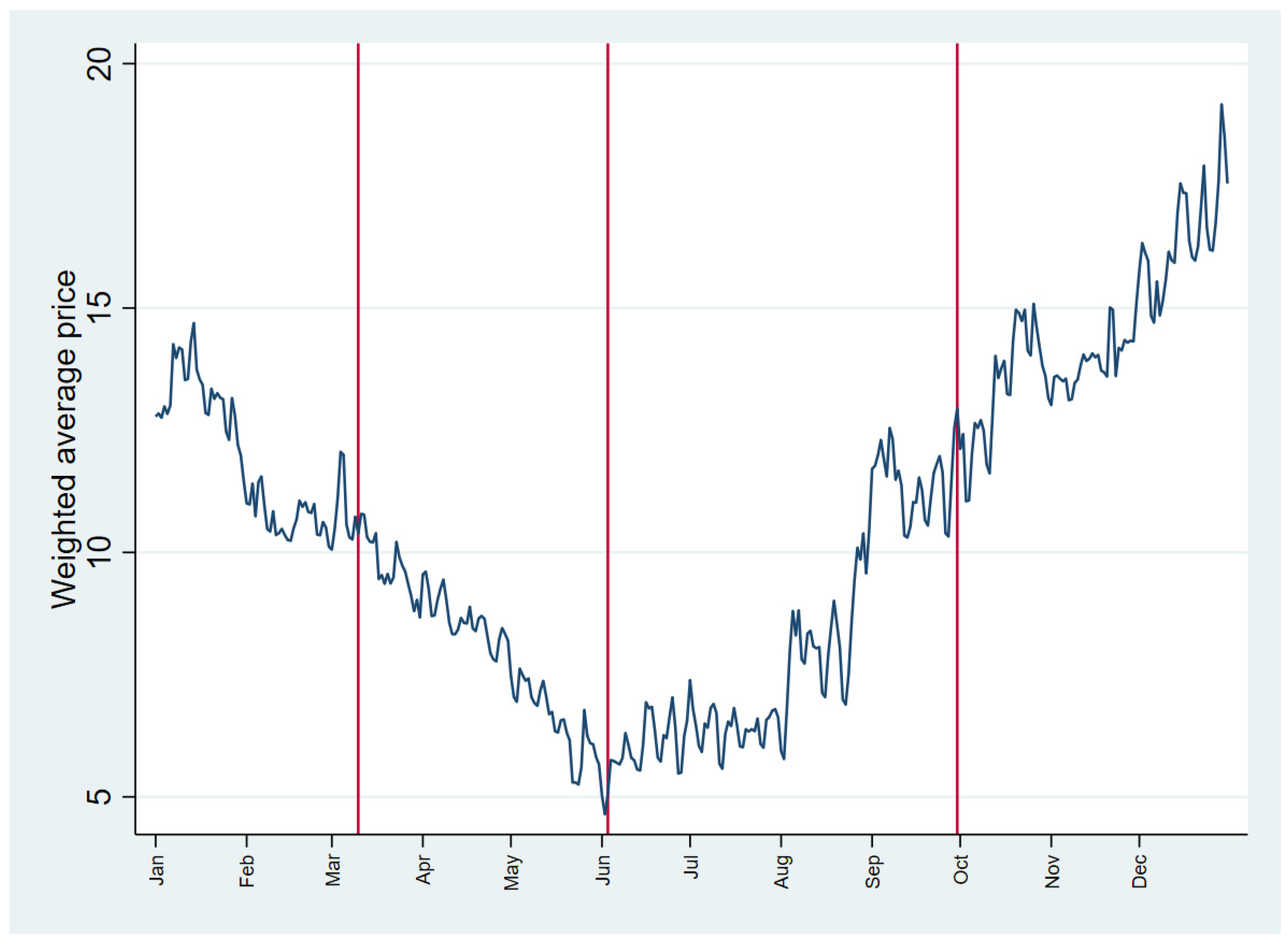
An analysis of energy source price dynamics needs also to be undertaken in order to explain the sudden change in the price elasticity of electricity demand. The pattern of the average prices (weighted for the related volumes) of the contracts traded in the Italian gas market is shown in Figure 9. A downward trend was recorded from February and at the end of May prices reached the minimum values. The trend switched in June, prices started increasing and, by the end of 2020, they had far exceeded the values recorded in the pre-lockdown period.

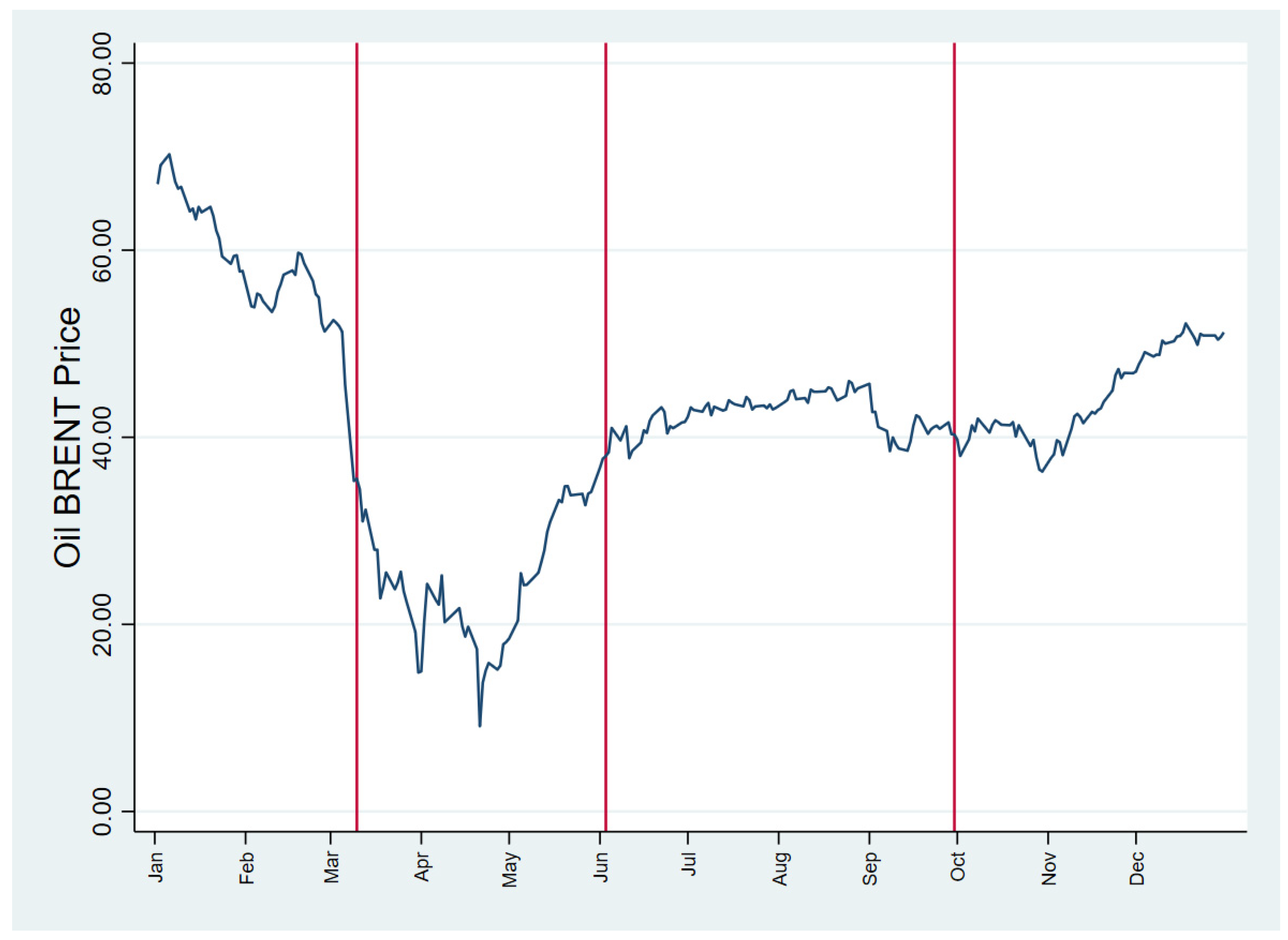
On the other hand, oil prices recorded a different dynamic, as shown in Figure 10, which depicts the time pattern of the daily BRENT crude oil prices recorded during 2020. From the beginning of the year a declining trend was recorded, reaching the minimum value of about 10 dollars per barrel in the middle of April. The recovery began in the second half of April and, at the beginning of June, prices leveled off on values between 40 and 55 dollars per barrel. However, at the end of the year, oil prices were far below their usual values.

We wanted to analyze if the COVID pandemic affected the price responsiveness of electricity demand.

Again, we applied a linear regression model where the elasticities were the dependent variables regressed on variables expressing the main phenomena related to the COVID pandemic (Health Var.), such as hospitalizations and the reduction in mobility due to lockdown measures (Mobility Var.).

Variables defining the health situation at national level were the daily number of people hospitalized with COVID symptoms (Hosp.), the daily number of people in intensive care (Int. Care) and the daily variation in the total number of positive cases (Tot. Positive). All these health variables were derived from the database provided by The National Institute of Health. Regressors representative of the stringency of the lockdown measures were instead the percentage variations in station (Stat. Mob.) and workplace mobility (Work Mob.) from the baseline period (15 January 2020–6 February 2020). These variables were sourced from the Google Mobility database. We employed as control variables several structural dummies for days of the week, months and seasons that captured the differences in price responsiveness due to cyclical and weather phenomena.

$${\epsilon }_t={\beta }_1 Health Var{.}_t+{\beta }_2 Mobility Var{.}_t+{\sum }_k{\gamma }_k{d}_k+u_t$$

(6)

The structural break highlighted in the graphs is tested using Chow Test. We identify the break in the dynamic of elasticity on 1 October and we split the sample into two groups according to this date. The first group corresponds to a dummy variable q1 equal to one until the 30 September. The second group corresponds to a dummy variable q₂ equal to one for all elasticities computed after 30 September. We then run the following regression:

$${\epsilon }_t={\beta }_{1,1}\left(q_1\ast Healt Var{.}_t\right)+{\beta }_{1,2}\ast \left(q_2\ast Healt Var{.}_t\right)+{\beta }_{2,1}\left(q_1\ast Mobility Var{.}_t\right)+{\beta }_2\left(q_2 Mobility Var{.}_t\right)+{\sum }_k{\gamma }_{k,1}\left(q_1\ast d_k\right)+{\gamma }_{k,2}\left(q_2\ast d_k\right)+u_t$$

(7)

where all variables are interacted with the two dummies and we test the equalities of coefficients.

Table 11. Chow Test Results.

$H_0: {\beta }_{1,1}={\beta }_{1,2}; {\beta }_{2,1}={\beta }_{2,2}; {\gamma }_{k,1}={\gamma }_{k,2} \forall k=1,\dots K$	F (8, 7472) = 1403.43
$H_1: {\beta }_{1,1}\ne {\beta }_{1,2}; {\beta }_{2,1}\ne {\beta }_{2,2}; {\gamma }_{k,1}\ne {\gamma }_{k,2} \forall =1,\dots K$	Prob > F = 0.0000

reports the F test statistics for the Chow test. The F test leads to rejection of the null hypothesis that the two groups share the same coefficient estimates, and, therefore, the two samples are from two different probability distributions with different mean.

The F test’s results lead us to perform six different regressions for the two subsamples. Results are shown in

Table 12. Regression Results: Period between 1 January–30 September.

	M(1)	M(2)	M(3)	M(4)	M(5)	M(6)
	b/s.d.	b/s.d.	b/s.d.	b/s.d.	b/s.d.	b/s.d.
Hosp.	−0.000000055 ***	−0.000000125 ***
	0.0000000153	0.0000000167
Int. Care			−0.000000532 ***	−0.000000920 ***
			(0.0000000997	(0.000000105
Tot. Positive					0	−0.000000182 ***
					0.0000000561	0.0000000576
Work Mob.	−0.0000168 ***		−0.0000215 ***		0.00000645
	0.0000503		0.00000483		0.00000405
Stat. Mob.		−0.0000507 ***		−0.0000514 ***		−0.0000235 ***
		0.00000606		(0.00000562		0.00000461
d.March	0.001894 ***	0.001168 ***	0.002053 ***	0.001345 ***	0.001758 ***	0.001217 ***
	0.000324	0.000335	0.000325	0.000335	0.000323	0.000338
d.April	0.002738 ***	0.002397 ***	0.002640 ***	0.001866 ***	0.001952 ***	0.000963 **
	0.000398	0.000398	(0.000365	0.000376	0.000356	0.000389
d.May	0.002865 ***	0.002400 ***	0.002549 ***	0.001725 ***	0.002391 ***	0.001535 ***
	0.000314	0.000318	(0.000306	0.000321	0.000353	0.000379
d.June	0.002702 ***	0.002514 ***	0.002540 ***	0.002255 ***	0.002615 ***	0.002286 ***
	0.000295	0.000292	(0.000296	0.000294	0.000308	0.000308
d.July	0.002531 ***	0.002583 ***	0.002452 ***	0.002511 ***	0.002586 ***	0.002545 ***
	0.000292	0.000287	(0.000292	0.000287	0.000293	0.000289
d.August	0.001813 ***	0.002143 ***	0.001675 ***	0.002062 ***	0.002022 ***	0.002150 ***
	0.000307	0.000287	(0.000307	0.000287	0.000301	0.000289
d.September	−0.007554 ***	−0.007147 ***	−0.007637 ***	−0.007263 ***	−0.007505 ***	−0.007320 ***
	0.000293	0.000292	0.000293	(0.000289	0.000293	0.000293
d.Tuesday	−0.000514 ***	−0.000477 ***	−0.000516 ***	−0.000477 ***	−0.000537 ***	−0.000563 ***
	0.000162	0.000161	0.000161	0.00016	0.000163	0.000163
d.Wednesday	−0.00026	−0.000292 *	−0.00025	−0.000278 *	−0.000282*	−0.000319 *
	0.000163	0.000162	0.000163	0.000162	0.000164	0.000164
d.Thursday	−0.0001	−0.00014	−0.000096	−0.00012	−0.00097	−0.00011
	0.000163	0.000162	0.000163	0.000162	0.000163	0.000163
d.Friday	0.000177	0.000162	0.000184	0.000188	0.000192	0.00018
	0.000163	0.000162	0.000163	0.000162	0.000163	0.000163
d.Saturday	−0.000045	0.00017	0.000014	0.000204	−0.00014	−0.000017
	0.000169	0.000168	0.000169	0.000167	0.000168	0.000167
d.Sunday	0.000720 ***	0.000676 ***	0.000847 ***	0.000693 ***	0.000476 **	0.000520 ***
	0.000208	0.000169	0.000206	0.000168	0.000198	0.000169
Constant	−0.009640 ***	−0.010409 ***	−0.009696 ***	−0.010416 ***	−0.009497 ***	−0.009852 ***
	0.000291	0.000306	0.00029	0.000302	0.000288	0.000296

Note: standard deviations in the second row in italics. * p < 0.10, ** p < 0.05, *** p < 0.01.

and

Table 13. Regression Results: Period between 1 October–31 December.

	M(1)	M(2)	M(3)	M(4)	M(5)	M(6)
	b/s.d.	b/s.d.	b/s.d.	b/s.d.	b/s.d.	b/s.d.
Hosp.	−0.00000015 **	−0.00000016 **
	0.00000007	0.00000008
Int. Care			−0.00000761 ***	0.00000188 ***
			0.000001	0.000001
Tot. Positive					−0.0000000454	−0.0000000389
					0.0000000367	0.0000000368
Work Mob.	0.000308 ***		0.000308 ***		0.000303 ***
	0.00003		0.00003		0.00003
Stat. Mob.		0.000367 ***		0.000375 ***		0.000337 ***
		0.000035		0.000035		0.000033
d.November	0.166493 ***	0.166968 ***	0.164738 ***	0.165973 ***	0.162923 ***	0.170827 ***
	0.00373	0.00373	0.003655	0.003656	0.003157	0.003288
d.December	0.152931 ***	0.152706 ***	0.151418 ***	0.151692 ***	0.148774 ***	0.155281 ***
	0.003626	0.003621	0.003589	0.003583	0.003172	0.003312
d.Tuesday	0.026777 ***	0.025981 ***	0.026749 ***	0.025954 ***	0.026869 ***	0.026207 ***
	0.001172	0.001171	0.001173	0.00117	0.00118	0.001179
d.Wednesday	0.032459 ***	0.032448 ***	0.032418 ***	0.032403 ***	0.032459 ***	0.032670 ***
	0.001174	0.001173	0.001175	0.001172	0.001176	0.001174
d.Thursday	0.032863 ***	0.032908 ***	0.032858 ***	0.032865 ***	0.033118 ***	0.033180 ***
	0.001151	0.001151	0.001152	0.00115	0.001179	0.001178
d.Friday	0.033272 ***	0.033361 ***	0.033245 ***	0.033289 ***	0.033419 ***	0.033640 ***
	0.001174	0.001174	0.001176	0.001174	0.001193	0.001193
d.Saturday	0.024276 ***	0.024903 ***	0.024244 ***	0.024791 ***	0.024523 ***	0.025361 ***
	0.001175	0.001172	0.001177	0.001172	0.001214	0.001208
d.Sunday	−0.004999 ***	−0.000979	−0.004949 ***	−0.001	−0.004450 ***	−0.000733
	0.001213	0.001171	0.001214	0.001169	0.001272	0.001218
Constant	−0.243751 ***	−0.246370 ***	−0.243944 ***	−0.246259 ***	−0.244284 ***	−0.246467 ***
	0.003285	0.003237	0.003285	0.003234	0.003284	0.003241

Note: standard deviations in the second row in italics. * p < 0.10, ** p < 0.05, *** p < 0.01.

. In the first two models we employ as health variable the number of people hospitalized (Hosp.). Models differ in the mobility variables; we use the Work Mob. variation in the first and the Stat. Mob. variation in the second. In the third and fourth models we change the health variable with Int. Care. In the last two models we replace the health variable with Tot. Positive.

Table 12 shows results for the first regression referring to the period 1 January–30 September. In all six different models the health variables always have a negative sign, when significant.

This means that the worse the health situation, the more negative the estimates of elasticity are. That is, the worsening of the health situation at national level made the demand for electricity even more elastic. The effect of the health variables on the responsiveness of the demand price is however very low. For instance, increasing the total number of hospitalized patients by one turns into in an increase (in absolute value) in the elasticity of demand between −5.5 × 10⁻⁸, in the model with Work Mob., and −1.25 × 10⁻⁷ in the model with Stat. Mob. The greatest effect on elasticity comes from the number of patients in intensive care (Int. Care), whose coefficient ranges between −5.32 × 10⁻⁷ and −9.2 × 10⁻⁷ in the model with Work. Mob. and Stat. Mob., respectively. In the last two models, the Tot. Positive health variable is significant only in the model associated with the mobility of the stations, with a value equal to −1.82 × 10⁻⁷.

Looking instead at the mobility variables, their coefficients are also always negative when significant. This means that an increase in either workplace or station mobility made the values of the elasticity estimates even more negative. Conversely, a shrinkage of mobility increased the value of elasticity, bringing it closer to zero. In other words, the sharp reduction in mobility caused by the lockdown restrictions made the demand for electricity more inelastic. This was due to the strong contraction in demand from big consumers that changed the composition of loads, increasing the share of energy consumption for essential industrial activities which could not be interrupted and, therefore, that were more inelastic. The coefficients relating to workplace mobility lie between −1.68 × 10⁻⁵ and −2.15 × 10⁻⁵. The effects of station mobility on elasticity are greater (in absolute value), and between −2.35 × 10⁻⁵ and −5.14 × 10⁻⁵.

Table 13 shows the regression results referring to the period 1 October–30 December.

The health variables confirm their negative coefficients when significant. The daily variation of positive cases is no longer significant. Since the end of the summer, the increase in the number of positive cases was in fact considered a marginal factor, because COVID-19 had become increasingly endemic.

The public authorities, on the other hand, were looking with great concern at the increase in the number of hospitalized patients, whose acceleration could once again impose a health emergency and a collapse of hospitals, unable to accommodate an increasing number of severely ill patients. This phenomenon provides an analogy with the non-significance of Tot Positive on the performance of economic activities and, in turn, on the elasticity of the electricity demand. The other two health variables (Hosp. and Int. Care) show instead coefficients higher than those of the previous period (in absolute value), ranging from −1.6 × 10⁻⁷ to −1.5 × 10⁻⁷ for Hosp. and 0 to 10 for Int. Care. This highlights how the number of hospitalized patients (in intensive care and not) made elasticity even more negative and, in turn, the electricity demand more elastic. The risk of hospital congestion has in fact conditioned the pace of economic activities at the national level, leading local authorities to fine-tune specific measures to again constrain the spread of disease.

The coefficients of variables proxying the changes in mobility are significant, but they changed sign, becoming positive in the last period of the year. It is noteworthy that, by the second wave of the pandemic, many business and economic activities had already changed their operational schemes, introducing systematic forms of smart and tele working. Therefore, they had been ready to face new restrictions and lockdowns, avoiding the dramatic slowdown of the economy and the sharp contraction of energy demand.

4. Conclusions

In this paper we investigated the impact of the COVID-19 pandemic shock on the price responsiveness of Italian electricity demand. The restrictions governments worldwide undertook to contain the spread of the pandemic affected the electricity demand loads. We showed that the level and the profile of electricity loads dramatically shrank during the period of heavy lockdown. Furthermore, we highlighted that the composition of the loads changed, recording growth in share of residential demand and drastic decline in share of big consumers, due to industry closedowns and travel ban. All this necessarily resulted in a change in the elasticity of demand that we investigated.

Results of the study highlighted that, during the heavy lockdown period, price demand elasticity shrank. Indeed, businesses that remained operational referred to essential activities whose electricity demand could not be adjusted during the day according to the hourly equilibrium prices expected in the DAM. We also showed that the last period of the year, characterized by the recrudescence of the pandemic and weaker restrictions on mobility, recorded a structural break on the dynamic of elasticity, which increased dramatically. This structural break has been explained with the reversal trend of natural gas and oil prices, which consistently rose from the end of summer, and the changes in marginal technologies, with gas- and coal-based plants increasing their frequency of being closing technology defining the clearing price.

The analysis of the dynamics of price elasticity showed that, in the first subperiod, the health variables were significant and the spread of the disease in terms of positive cases and hospitalizations increased the price responsiveness of electricity demand. The variables representing the changes in mobility were also significant with negative coefficients, highlighting that the reduction in mobility made demand more rigid. The strong contraction in demand from big consumers changed the composition of loads, increasing the share of energy consumption for those essential activities which could not be interrupted and, in turn, that were more rigid. After the structural break, in the second subperiod, the health variables continued to be significant with negative coefficients, except for the number of positive cases. These findings highlighted that only hospitalizations and the linked risk of hospital congestion were the significant variables that affected the pace of economic activities and, in turn, energy demand. The coefficients relating to the mobility variables became instead positive. A reduction in mobility due to restrictive measures made elasticity even more negative and, in turn, demand even more elastic. Many economic activities had already changed their operational schemes, by reorganizing human resources and introducing smart working. Therefore, many businesses were ready to face the new challenges of the pandemic second wave, avoiding the drastic decline of the economy and a sharp contraction in energy demand.

To summarize, the impacts due to the pandemic posed various challenges and consequently opened the door for new opportunities and improvements in the power sector. Utilities were challenged to overcome the normal scenarios and they had to be prepared to combat new, unforeseen threats. One of the most effective strategies the electricity sector should undertake is investing in improved system flexibilities to tackle the technical issues raised by the reductions and changes of electricity loads. We acknowledge that this work has some limitations, assuming an atomistic competitive market. Further work may include assumptions on strategic behavior and test for oligopolistic market power. As a final recommendation for the future, we think that this approach can be useful for the regulators to study more in depth the characteristics of demand. In fact, as demand elasticity plays a pivotal role in defining load profiles, this study can provide a new methodological framework for both regulators and utilities to monitor demand price responsiveness in the Italian wholesale electricity market.

References

- Bahmanyar, A.; Estebsari, A.; Ernst, D. The impact of different COVID-19 containment measures on electricity consumption in Europe. Energy Res. Soc. Sci. 2020, 68, 101683. [Google Scholar] [CrossRef]
- Malkawi, S.; Kiwan, S.; Alzghoul, S. Impact of COVID-19 Response Measures on Electricity Sector in Jordan. Energies 2022, 15, 3810. [Google Scholar] [CrossRef]
- Samara, F.; Abu-Nabah, B.A.; El-Damaty, W.; Al Bardan, M. Assessment of the Impact of the Human Coronavirus (COVID-19) Lockdown on the Energy Sector: A Case Study of Sharjah, UAE. Energies 2022, 15, 1496. [Google Scholar] [CrossRef]
- Sztorc, M. The Implementation of the European Green Deal Strategy as a Challenge for Energy Management in the Face of the COVID-19 Pandemic. Energies 2022, 15, 2662. [Google Scholar] [CrossRef]
- AEMO. Quarterly Energy Dynamics Q1 2020, Market Insights and WA Market Operations. Australian Energy Market Operator, 1–44. 2020. Available online: https://aemo.com.au/-/media/files/major-publications/qed/2020/qed-q1-2020.pdf?la=en&hash=490D1E0CA7A21DB537741C5C18F2FF0A (accessed on 30 June 2022).
- Batsas, M. Public Transport Authorities and COVID-19, Impact and Response to a Pandemic. International Association of Public Transport, Australia/New Zealand, 1–7. 2020. Available online: https://australia-newzealand.uitp.org/sites/default/files/V1_COVID-19%20impacts_AJ_v03.pdf (accessed on 30 June 2022).
- Abu-Rayash, A.; Dincer, I. Analysis of mobility trends during the COVID-19 coronavirus pandemic: Exploring the impacts on global aviation and travel in selected cities. Energy Res. Soc. Sci. 2020, 68, 101693. [Google Scholar] [CrossRef]
- Wu, S.; Zhou, W.; Xiong, X.; Burr, G.; Cheng, P.; Wang, P.; Niu, Z.; Hou, Y. The impact of COVID-19 lockdown on atmospheric CO2 in Xi’an, China. Environ. Res. 2021, 197, 111208. [Google Scholar] [CrossRef] [PubMed]
- Ahn, D.; Salawitch, R.; Canty, T.; He, H.; Ren, X.; Goldberg, D.; Dickerson, R. The U.S. power sector emissions of CO2 and NOx during 2020: Separating the impact of the COVID-19 lockdowns from the weather and decreasing coal in fuel-mix profile. Atmospheric Environ. X 2022, 14, 100168. [Google Scholar] [CrossRef]
- Farrow, H. Commercial Down v Residential Up: COVID-19’s Electricity Impact. Energy Insider, Energy Networks Australia. 2020. Available online: https://www.energynetworks.com.au/news/energy-insider/2020-energy-insider/commercial-down-v-residential-up-covid-19s-electricity-impact/ (accessed on 30 June 2022).
- ENEDIS. Sector-Wise Annual Production at Department-Level. Open Data. 2020. Available online: https://data.enedis.fr/explore/?sort=modified (accessed on 30 June 2022).
- Elavarasan, R.M.; Shafiullah, G.; Raju, K.; Mudgal, V.; Arif, M.; Jamal, T.; Subramanian, S.; Balaguru, V.S.; Reddy, K.; Subramaniam, U. COVID-19: Impact analysis and recommendations for power sector operation. Appl. Energy 2020, 279, 115739. [Google Scholar] [CrossRef] [PubMed]
- Li, L.; Meinrenken, C.J.; Modi, V.; Culligan, P.J. Impacts of COVID-19 related stay-at-home restrictions on residential electricity use and implications for future grid stability. Energy Build. 2021, 251, 111330. [Google Scholar] [CrossRef] [PubMed]
- IEA. Global Energy Review 2020: The Impacts of the COVID-19 Crisis on Global Energy Demand and CO2 Emissions. 2020. Available online: https://www.iea.org/reports/global-energy-review-2020 (accessed on 30 June 2022).
- EIA—U.S. Energy Information Administration. Short-Term Energy Outlook, May-2020, 1–51. (STEO). 2020. Available online: https://www.eia.gov/outlooks/steo/pdf/steofull.pdf (accessed on 30 June 2022).
- Şahin, U.; Ballı, S.; Chen, Y. Forecasting seasonal electricity generation in European countries under Covid-19-induced lockdown using fractional grey prediction models and machine learning methods. Appl. Energy 2021, 302, 117540. [Google Scholar] [CrossRef]
- Halbrügge, S.; Buhl, H.U.; Fridgen, G.; Schott, P.; Weibelzahl, M.; Weissflog, J. How Germany achieved a record share of renewables during the COVID-19 pandemic while relying on the European interconnected power network. Energy 2022, 246, 123303. [Google Scholar] [CrossRef]
- Euroeletric. Impact of COVID-19 on costumers and society. In Recommendations from the European Power Sector; Eurelectric Recommendations Paper Series; Euroeletric: Brussels, Belgium, 2020; pp. 1–35. [Google Scholar]
- Rugani, B.; Caro, D. Impact of COVID-19 outbreak measures of lockdown on the Italian Carbon Footprint. Sci. Total Environ. 2020, 737, 139806. [Google Scholar] [CrossRef] [PubMed]
- Zhong, H.; Tan, Z.; He, Y.; Xie, L.; Kang, C. Implications of COVID-19 for the electricity industry: A comprehensive review. CSEE J. Power Energy Syst. 2020, 6, 489–495. [Google Scholar]
- Apadula, F.; Bassini, A.; Elli, A.; Scapin, S. Relationships between meteorological variables and monthly electricity demand. Applied Energy 2012, 98, 346–356. [Google Scholar] [CrossRef]
- Contreras, J.; Espinola, R.; Nogales, F.; Conejo, A. ARIMA models to predict next-day electricity prices. IEEE Trans. Power Syst. 2003, 18, 1014–1020. [Google Scholar] [CrossRef]
- Gonzalez, J.P.; Roque, A.M.S.; Perez, E.A. Forecasting functional time series with a new Hilbertian ARMAX model: Application to electricity price forecasting. IEEE Trans. Power Syst. 2017, 33, 545–556. [Google Scholar] [CrossRef]
- Babu, C.N.; Reddy, B.E. A moving-average filter based hybrid ARIMA–ANN model for forecasting time series data. Appl. Soft Comput. 2014, 23, 27–38. [Google Scholar] [CrossRef]
- Wang, Q.; Li, S.; Li, R. Forecasting energy demand in China and India: Using single-linear, hybrid-linear, and non-linear time series forecast techniques. Energy 2018, 161, 821–831. [Google Scholar] [CrossRef]
- Garcia, R.; Contreras, J.; van Akkeren, M.; Garcia, J. A GARCH forecasting model to predict day-ahead electricity prices. IEEE Trans. Power Syst. 2005, 20, 867–874. [Google Scholar] [CrossRef]
- Qu, H.; Duan, Q.; Niu, M. Modeling the volatility of realized volatility to improve volatility forecasts in electricity markets. Energy Econ. 2018, 74, 767–776. [Google Scholar] [CrossRef]
- Jan, F.; Shah, I.; Ali, S. Short-Term Electricity Prices Forecasting Using Functional Time Series Analysis. Energies 2022, 15, 3423. [Google Scholar] [CrossRef]
- Shah, I.; Lisi, F. Forecasting of electricity price through a functional prediction of sale and purchase curves. J. Forecast. 2020, 39, 242–259. [Google Scholar] [CrossRef]
- Bollino, C.A. Gaids: A generalised version of the almost ideal demand system. Econ. Lett. 1987, 23.2, 199–202. [Google Scholar] [CrossRef]
- Deaton, A.; Muellbauer, J. An almost ideal demand system. Am. Econ. Rev. 1980, 70, 312–326. [Google Scholar]
- D’Errico, M.C.; Bollino, C.A. Bayesian Analysis of Demand Elasticity in the Italian Electricity Market. Sustainability 2015, 7, 12127–12148. [Google Scholar] [CrossRef] [Green Version]
- Bigerna, S.; Bollino, C.A. Electricity Demand in Wholesale Italian Market. Energy J. 2014, 35, 25–46. [Google Scholar] [CrossRef]
Figure 1.
Flowchart summarizing the main stages of the study.
Figure 2.
Market clearing outcomes in the DAM on the 22 September 2020; 12 a.m. The green line represents the aggregate electricity supply, the orange line the aggregate electricity demand.
Figure 3.
Empirical Demands in the DAM. 9 March and 16 March 2020. Hour: 12 a.m. and 12 p.m. Figure on the left represents the two aggregated demands recorded at 12 a.m. Figure on the right represents the two aggregated demands recorded at 12 p.m.
Figure 4.
Weekly Load Profiles for the Third Week of March 2019 and 2020.
Figure 5.
Relative Annual Variation (2020 vs. 2019) of Market Equilibrium Prices (PUN)-Weekly Average.
Figure 6.
Relative Annual Variation (2020 vs. 2019) of Equilibrium Quantity (Total Purchases)-Weekly Average.
Figure 7.
Hourly elasticity estimates for the hours 1 a.m.–12 a.m., 2020.
Figure 8.
Hourly elasticity estimates for the hours 1 p.m.–12 p.m., 2020.
Figure 9.
Daily Gas Weighted Average Price in the Italian Gas Market, 2020. Note: The weighted price is expressed in terms of euro/MWh. Source: Italian Day-Ahead Gas Market.
Figure 10.
Daily BRENT Oil Price, 2020. Source: Federal Reserve Economic Data; https://fred.stlouisfed.org. Crude Oil Prices: Brent-Europe, Dollars per Barrel, Daily, Not Seasonally Adjusted (accessed on 1 June 2022).