Modelling the Potential Impact of Stigma on the Transmission Dynamics of COVID-19 in South Africa

Abstract

The COVID-19 pandemic continues to be a problem in South Africa. Individuals affected and infected by the disease suffer from stigma resulting in increased COVID-19 infections. In this paper, we developed a mathematical model to assess the effects of stigma on COVID-19 in South Africa, using low, moderate, and high stigma regimes in the population. The mathematical model was analysed and the basic reproduction number, R₀, of the COVID-19 model with stigma was determined. The model was then fitted to data of the four COVID-19 waves for the new daily infected cases, and the estimated parameter values from different waves are presented. The effects of stigma on COVID-19 waves were examined using the four stigma regimes (high, moderate, low, and stigma-free regimes). Our results revealed that stigma is instrumental in the increase in the number of COVID-19 infections. It is also a significant contributor to sustaining COVID-19 in the population and probably in other infectious diseases such as HIV/AIDS and sexually transmitted diseases. The results obtained can influence policy directions with respect to stigma and its impact on the transmission dynamics of diseases.

1. Introduction

Coronavirus (COVID-19) is an infectious disease caused by the Severe Acute Respiratory Syndrome Coronavirus 2 (SARS-CoV-2) that was not previously observed within a population or geographic location [1]. The pandemic dramatically changed peoples’ lives worldwide since it first appeared in Wuhan, China, at the beginning of December 2019 [2]. People’s lives have been negatively impacted by COVID-19-related suffering and lockdowns at community and household levels [3]. Lockdown regulations radically changed social contact by replacing face-to-face meetings with virtual meetings to reduce the spread of COVID-19. Social distancing, frequent hand washing, and the use of face masks in public are some of the most critical health behaviors to reduce virus transmission from an infectious patient to others [4,5].

Stress caused by lockdowns, and fear of being infected fuelled the rise of stigma in local communities [2]. The stigma of origin is a Greek word that refers to a marking burned into the skin of criminals, enslaved people, or traitors to visibly identify them as ‘blemished’ or ‘morally polluted persons’. These individuals were to be avoided, especially in public places [6]. Pescosolido [7] defined stigma as a sign of disgrace that sets a person apart from others. Stigma also involves negative attitudes or discrimination against someone based on a distinguishing characteristic such as obesity, mental illness, health condition, or disability [8]. According to Campbell and Deacon [9], there are three main types of stigma: enacted stigma, felt stigma, and tribal stigma. Enacted stigma, also known as external deformities, entails the experience of unfair treatment by others due to their perceived perception of an individual. Felt stigma, also known as internal stigma, refers to the shame and expectation of discrimination that prevents people from talking about their condition and stops them from seeking help [10]. Tribal stigma refers to shame and discrimination affiliated with a specific race, ethnicity, religion, etc. [9]. Stigma may result in delaying or avoiding treatment and seeking access to health services, which compromises the outcome of an individual’s medical condition [11], and, in the worst cases, in individuals dying before reaching health facilities. Stigma correlates with a lack of understanding of how COVID-19 spreads, a need to blame someone, fears about disease and death, and social media [12]. The stigma associated with COVID-19 is based on the fact that there is still information that is not known about the disease and misinformation driven by social media [13].

Differential equations provide remarkable essential tools to fight diseases by understanding and predicting the dynamics of infectious diseases under several distinct circumstances [14]. It is one of the most significant branches of mathematics that has been used to model different systems and processes [15]. Additionally, the theory of arbitrary order differential equations received extensive popularity due to its vast applicability in various branches of science and engineering [16].

Mathematical modeling of the epidemiology of COVID-19 in South Africa has recently become a powerful tool to study the dynamics of the pandemic and the importance of various control strategies so as to advise public health policymakers who aim to construct suitable intervention programs to fight the spread of COVID-19. Mukandavire et al. [17] looked at quantifying early COVID-19 outbreak transmission in South Africa and vaccine efficacy scenarios. They discovered that a highly efficacious vaccine would have been required to contain COVID-19 in South Africa. Nyabadza et al. [18] looked at modelling the potential impact of social distancing on the COVID-19 epidemic in South Africa. Their results showed that an increase in social distancing would decrease the spread of COVID-19. Gatyeni et al. [19] looked at the application of optimal control to the dynamics of COVID-19 disease in South Africa. Their numerical findings suggest that the joint implementation of effective mask usage, physical distancing, and active screening and testing, are effective measures that can be used to curtail the spread of the disease in the human population.

The effects of stigma on infectious diseases such as leprosy and tuberculosis (TB) have been studied [20,21], but very few studies have looked at how stigma impacts the ongoing COVID-19 pandemic. To this end, it is important to look at how different levels (regimes) of stigma impacted the four waves of the pandemic in South Africa. Those studies indicate that stigma does indeed play a role in increasing the number of infected individuals. It was demonstrated that the disease prevalence and incidence were high when stigma was high and declined gradually when the combination of both treatment and a health campaign was implemented. Thus, assessing the effects of stigma in stigmatised individuals is essential to determine its veracity towards the progression of COVID-19 and in devising control methods. Additionally, according to [22], COVID-19 caused stigma and discrimination against certain groups across the continent, including South Africa. When COVID-19 began to spread, people suffered discrimination and stigma as they were blamed for the spread of COVID-19. In some townships in South Africa, for instance, families of those who tested positive for COVID-19 experienced ill-treatment and discrimination due to the stigma associated with the virus. In this study, we thus proposed a simple mathematical model for the transmission dynamics of COVID-19 that can account for the effects of stigma to determine the potential impact of stigma on the dynamics of COVID-19 in South Africa. In particular, we classified stigma as either low, moderate, or high and determined how the number of infections was impacted by the different levels of stigma for the different waves of COVID-19 experienced in South Africa.

The paper is arranged as follows: in the next section, the model is formulated. Section 3 presents the model properties and the model analysis is presented in Section 4. In Section 5, simulations and a sensitivity analysis are presented and the last section concludes the paper.

2. Model Formulation

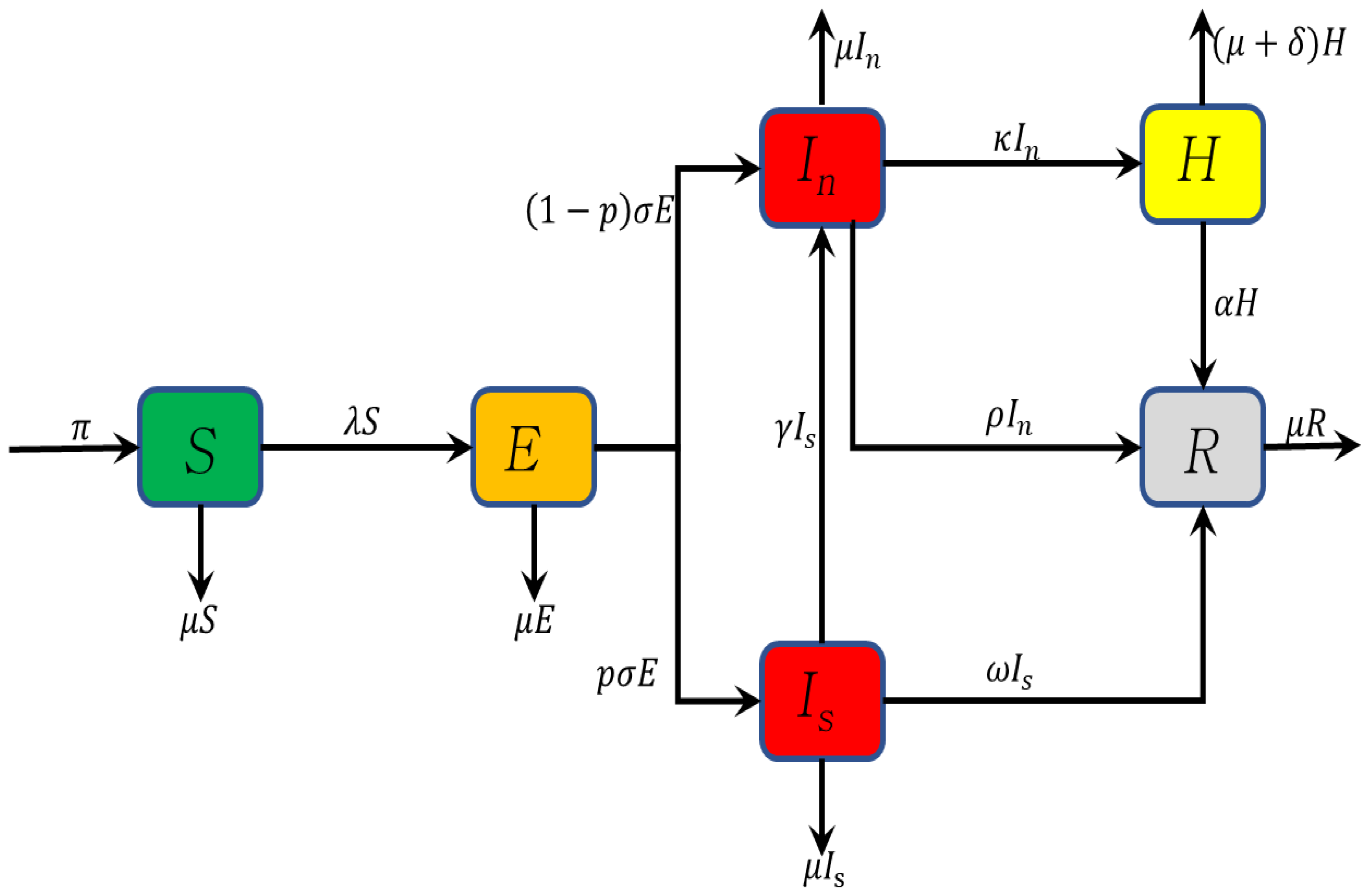
We proposed a model with the following six compartments: susceptible, exposed, infectious, hospitalized, and recovered individuals where the infectious population is divided into two, namely stigmatised and unstigmatised infectious populations. The susceptible individuals $S\left(t\right)$ are recruited at a constant rate $\pi$, where these individuals can become infected and move into the exposed class $E\left(t\right)$. We assume that exposed individuals become symptomatic at a rate $\sigma$. Some individuals with symptomatic infection choose to disclose their COVID-19 status and move to the unstigmatised individuals $I_n\left(t\right)$. In contrast, others choose to conceal their COVID-19 status and move to the stigmatised class $I_s\left(t\right)$ to avoid being discriminated against by the community. This is modelled by the parameter p, where $0<p<1$, with p being the proportion of infected that are stigmatised. We assume that those who initially conceal their COVID-19 illness can move to the $I_n\left(t\right)$ population at a rate $\gamma$, either by changing their minds, or disclosing their COVID-19 condition, thereby delaying access to health facilities. Individuals in $I_n\left(t\right)$ are hospitalized or recover at a rate $\kappa$ or $\rho$, respectively. Individuals in $I_s\left(t\right)$ recover at a rate $\omega$. Hospitalized individuals recover at a rate $\alpha$. Individuals in all compartments are assumed to have a natural death rate $\mu$. Hospitalized individuals have an additional death rate $\delta$ caused by COVID-19 disease. We assume that disease induced deaths are only in the hospitalization class since the only recorded data cases for deaths are from the hospitals. The force of infection is given by

$$\begin{array}{c}\hfill \lambda \left(t\right)=\frac{\beta \left(I_s\left(t\right)+ϵI_n\left(t\right)\right)}{N\left(t\right)},\end{array}$$

(1)

where $\beta$ is the infection rate and $ϵ\in [0,1]$ is the modification parameter that measures the relative infectiousness of individuals in $I_n\left(t\right)$ compared to individuals in $I_s\left(t\right)$. The total population $N\left(t\right)$ is given by

$$N\left(t\right)=S\left(t\right)+E\left(t\right)+I_n\left(t\right)+I_s\left(t\right)+H\left(t\right)+R\left(t\right).$$

Based on the flow diagram, Figure 1, the model assumptions, and the parameter descriptions, the differential equations that represent the COVID-19 model are given by

$$\begin{array}{c}\hfill \left.\begin{array}{ccc}\hfill & \frac{dS}{dt}=\pi -(\mu +\lambda )S,\hfill & \\ \hfill & \frac{dE}{dt}=\lambda S-a_{1}E,\hfill & \\ \hfill & \frac{d{I}_n}{dt}=(1-p)\sigma E+\gamma I_s-a_2{I}_n,\hfill & \\ \hfill & \frac{d{I}_s}{dt}=p\sigma E-a_3{I}_s,\hfill & \\ \hfill & \frac{dH}{dt}=\kappa I_n-a_{4}H,\hfill & \\ \hfill & \frac{dR}{dt}=\rho I_n+\omega I_s+\alpha H-\mu R,\hfill & \end{array}\right\}\end{array}$$

(2)

where

$$a_1=\mu +\sigma ,a_2=\mu +\kappa +\rho ,a_3=\mu +\omega +\gamma ,a_4=\mu +\delta +\alpha ,$$

with positive initial conditions given by

$$\begin{array}{c}\hfill S\left(0\right)=S^0>0,E\left(0\right)=E^0\ge 0,I_n\left(0\right)=I_n^0\ge 0,\\ \hfill I_s\left(0\right)=I_s^0\ge 0,H\left(0\right)=H^0\ge 0,R\left(0\right)=R^0\ge 0.\end{array}$$

(3)

We define time, $t=0,$ to be the time when COVID-19 started in South Africa. The number of susceptible population is initially strictly greater than zero, given that before the start of the epidemic, there were no infected.

3. Model Properties

In this section, we show that our model is well-posed. To show the well-posedness of the model, we proved that all solutions of the system of equations (2) with positive initial conditions remained positive for all $t\ge 0$. We also showed that the solutions were bounded for all $t\ge 0$ in the positive region $\Omega$, where $\Omega$ is a biologically feasible region, and the model should be biologically meaningful. Thus, based on the biological analysis, the model system (2) will be considered in the region below:

$$\begin{array}{c}\hfill \Omega =\left\{(S,E,I_n,I_s,H,R)\in {\mathbb{R}}_{+}^6:0\le N\le \frac{\pi }{\mu }\right\}.\end{array}$$

(4)

This region is positively invariant with respect to the model system (2).

3.1. Positivity of Solutions of the Model

Since model (2) monitors the human population, all the state variables must be positive and the solutions to the model system (2) with positive initial conditions (3) should remain positive for $t\ge 0$. Here, we show that the solutions of model (2) remain positive in the positive orthant given any non-negative initial conditions.

Theorem 1.

For the given initial conditions in (3), the solutions of model system (2) remains positive for all $t>0$ in Ω.

Proof. 

Given that the initial conditions are all non-negative, the first equation of (2) gives

$$\begin{array}{c}\hfill \frac{dS}{dt}+(\mu +\lambda )S\ge 0,\end{array}$$

(5)

so that after integration we have

$$\begin{array}{c}\hfill S\left(t\right)\ge S\left(0\right)e^{-\left(\mu t+{\int }_0^t\lambda \left(\tau \right)d\tau \right)}>0,\forall t>0.\end{array}$$

Since the exponential function is positive and $S\left(0\right)>0$, it is guaranteed that the solution of $S\left(t\right)$ remains positive for all time $t\ge 0.$

The second equation of the model system (2) gives

$$\begin{array}{c}\hfill \frac{dE}{dt}+a_{1}E\ge 0,\end{array}$$

which gives

$$\begin{array}{c}\hfill E\left(t\right)\ge E\left(0\right)e^{-a_{1}t}>0,\forall t>0.\end{array}$$

Similarly, it can easily be shown that $I_n\left(t\right)\ge 0,I_s\left(t\right)\ge 0,H\left(t\right)\ge 0$ and $R\left(t\right)\ge 0$ for all time $t>0$ and completes the proof. □

3.2. Boundedness of Solutions

We have the following theorem to show that these solutions are uniformly unique:

Theorem 2.

The solutions of model system (2) with initial conditions (3) are contained in the region $\Omega .$

Proof. 

$$\begin{array}{c}\hfill \frac{dN}{dt}=\pi -\mu N-\delta H\le \pi -\mu N.\end{array}$$

(6)

The solution (6), obtained by separating variables and integrating is given by

$$\begin{array}{c}\hfill N\left(t\right)\le \frac{\pi }{\mu }-\left(\frac{\pi }{\mu }-N_0\right)e^{-\mu t},\end{array}$$

(7)

If $N_0<\frac{\pi }{\mu }$, then the upper bound of $N\left(t\right)$ is $\frac{\pi }{\mu }$ when $t\to \infty$ . If $N_0\ge \frac{\pi }{\mu }$, then $N\left(t\right)$ decreases to $\frac{\pi }{\mu }$ when $t\to \infty$ and approaches $\Omega$ asymptotically. Since N is the sum of all state space variables, each of the individual state variables is less or equal to $\frac{\pi }{\mu }$. Additionally, the positivity and boundedness of solutions ensure that $\Omega$ is a feasible region. Therefore, for the model system (2), the region $\Omega$ is positively invariant, and all solutions starting in $\Omega$ stay in $\Omega$. □

4. Model Analysis

In this section, the reproduction number is calculated, equilibrium points are computed, and an stability analysis is established.

4.1. Equilibrium Points

4.1.1. Disease Free Equilibrium Point

The model has equilibrium points obtained by setting the right-hand side of system (2) to zero so that

$$\begin{array}{c}\hfill \pi -(\mu +{\lambda }^{*})S^{*}=0,\end{array}$$

(8)

$$\begin{array}{c}\hfill {\lambda }^{*}{S}^{*}-a_1{E}^{*}=0,\end{array}$$

(9)

$$\begin{array}{c}\hfill (1-p)\sigma E^{*}+\gamma I_s^{*}-a_2{I}_n^{*}=0,\end{array}$$

(10)

$$\begin{array}{c}\hfill p\sigma E^{*}-a_3{I}_s^{*}=0,\end{array}$$

(11)

$$\begin{array}{c}\hfill \kappa I_n^{*}-a_4{H}^{*}=0,\end{array}$$

(12)

$$\begin{array}{c}\hfill \rho I_n^{*}+\omega I_s^{*}+\alpha H^{*}-\mu R^{*}=0.\end{array}$$

(13)

From Equation (11), express $I_s^{*}$ in terms of $E^{*}$

$$\begin{array}{c}\hfill I_s^{*}=Q_0{E}^{*},\mathrm{where}{Q}_0=\frac{p\sigma }{a_3}.\end{array}$$

(14)

Substituting (14) into (10), we get

$$\begin{array}{c}\hfill I_n^{*}=Q_1{E}^{*},\mathrm{where}{Q}_1=\frac{(1-p)\sigma +\gamma Q_0}{a_2}.\end{array}$$

(15)

From Equation (12), we have

$$\begin{array}{c}\hfill H^{*}=Q_2{E}^{*},\mathrm{where}{Q}_2=\frac{\kappa Q_1}{a_4}.\end{array}$$

(16)

Substituting Equations (14)–(16) in Equation (13), we have

$$\begin{array}{c}\hfill R^{*}=Q_3{E}^{*},\mathrm{where}{Q}_3=\frac{\rho Q_1+\omega Q_0+\alpha Q_2}{\mu }.\end{array}$$

(17)

From the force of infection in (1), we have

$$\begin{array}{c}\hfill {\lambda }^{*}=\frac{Q_4}{N^{*}}{E}^{*},\mathrm{where}{Q}_4=\beta (Q_0+ϵQ_1).\end{array}$$

(18)

Substituting (18) for ${\lambda }^{*}$ in Equation (9), we have

$$\begin{array}{c}\hfill \left(\frac{Q_4}{N^{*}}{S}^{*}-a_1\right)E^{*}=0.\end{array}$$

(19)

So, $E^{*}=0$ or

$$\begin{array}{c}\hfill \frac{S^{*}}{N^{*}}=\frac{1}{R_0},\mathrm{where}{R}_0=\frac{Q_4}{a_1}.\end{array}$$

(20)

Thus, when $E^{*}=0$ we obtain the disease free equilibrium points $\left(DFE\right)$, $E_0,$ given by

$$\begin{array}{c}\hfill E_0=\left(\frac{\pi }{\mu },0,0,0,0,0\right).\end{array}$$

(21)

4.1.2. Basic Reproduction Number

In epidemiological models, the basic reproduction number $R_0$ is the expected number of secondary cases produced by a typical infective individual in a completely susceptible population [23]. In this case, we evaluated $R_0$ to measure the average number of new individuals infected by COVID-19 generated by a single infected individual in a susceptible population. If $R_0<1$, on average, the infected individual produces less than one infection during their ability to initiate infection, and the disease will die out. Otherwise, if $R_0>1$, an infected individual produces more than one infected individual in a wholly susceptible community, and the disease persists. We used the next generation matrix method, see [23,24], to derive the basic reproduction number $R_0$ of the model. $R_0$ is defined to be the largest eigenvalue of the matrix $F{V}^{-1}$, with F representing the new infections matrix and $V^{-1}$ represents the inverse of the transfer matrix, V, so that

$$\mathrm{F}=\left(\begin{array}{cccc}0& \beta ϵ& \beta & 0\\ 0& 0& 0& 0\\ 0& 0& 0& 0\\ 0& 0& 0& 0\end{array}\right),\mathrm{V}=\left(\begin{array}{cccc}{a}_1& 0& 0& 0\\ -(1-p)\sigma & a_2& -\gamma & 0\\ -p\sigma & 0& a_3& 0\\ 0& -\kappa & 0& a_4\end{array}\right),$$

$$\mathrm{V}{}^{-1}=\left(\begin{array}{cccc}{\displaystyle \frac{1}{a_1}}& 0& 0& 0\\ {\displaystyle \frac{a_4\sigma \left(a_3(1-p)+p\gamma \right)}{a_1{a}_2{a}_3{a}_4}}& {\displaystyle \frac{1}{a_2}}& {\displaystyle \frac{\gamma }{a_2{a}_3}}& 0\\ {\displaystyle \frac{p\sigma }{a_1{a}_3}}& 0& {\displaystyle \frac{1}{a_3}}& 0\\ {\displaystyle \frac{\kappa \sigma \left(a_3(1-p)+p\gamma \right)}{a_1{a}_2{a}_3{a}_4}}& {\displaystyle \frac{\kappa }{a_2{a}_4}}& {\displaystyle \frac{\kappa \gamma }{a_2{a}_3{a}_4}}& {\displaystyle \frac{1}{a_4}}\end{array}\right),$$

$$\mathrm{and}\mathrm{FV}{}^{-1}=\left(\begin{array}{cccc}{\displaystyle \frac{\beta p\sigma }{a_1{a}_3}+\frac{\beta ϵ\sigma \left(a_3(1-p)+p\gamma \right)}{a_1{a}_2{a}_3}}& {\displaystyle \frac{\beta ϵ}{a_2}}& {\displaystyle \frac{\beta }{a_3}+\frac{\beta ϵ\gamma }{a_2{a}_3}}& 0\\ 0& 0& 0& 0\\ 0& 0& 0& 0\\ 0& 0& 0& 0\end{array}\right).$$

The basic reproduction number of COVID-19 with stigma is given by

$$\begin{array}{c}\hfill R_0=R_1+R_2,\end{array}$$

(22)

where

$$\begin{array}{c}\hfill R_1=\frac{\beta p\sigma }{a_1{a}_3},R_2=\frac{\beta \sigma ϵ}{a_1{a}_2{a}_3}\left(a_3(1-p)+p\gamma \right).\end{array}$$

(23)

The expression in $R_1$ represents the number of new COVID-19 infections generated by stigmatised infectious population $I_s$. It contains the product of transmission rate $\beta ,$ the fraction ${\displaystyle \frac{p\sigma }{a_1}}$ moving to stigmatised population $I_s$, and ${\displaystyle \frac{1}{a_3}}$ is the average time spent in the $I_s$ compartment. The expression in $R_2$ represents the number of new infections generated by the non-stigmatised infectious population $I_n$. The product of infectious rate due to non-stigmatisation is given by $\beta ϵ$, the fraction of exposed individuals moving to non-stigmatised population is given by ${\displaystyle \frac{\sigma (1-p)}{a_1}}$, and ${\displaystyle \frac{1}{a_2}}$ is the average time spent in the $I_n$ compartment. Following, Theorem 2, in [24], $E_0,$ is locally asymptotically stable whenever $R_0<1$ and unstable when $R_0>1$.

4.1.3. Endemic Equilibrium Point

The total population at equilibrium $N^{*}$ is given by

$$\begin{array}{c}\hfill N^{*}=S^{*}+Q_5{E}^{*},\mathrm{where}{Q}_5=1+Q_1+Q_0+Q_2+Q_3.\end{array}$$

(24)

Substituting (24) for $N^{*}$ in Equation (20), we have

$$\begin{array}{c}\hfill E^{*}=\frac{S^{*}(R_0-1)}{Q_5}.\end{array}$$

(25)

Substituting (18), (20), and (24) in Equation (8), we have

$$\begin{array}{c}\hfill S^{*}=\frac{\pi Q_5{R}_0}{\mu Q_5{R}_0+(R_0-1)Q_4}.\end{array}$$

(26)

Substituting (26) in (25), we have

$$\begin{array}{c}\hfill E^{*}=\frac{\pi R_0(R_0-1)}{\mu Q_5{R}_0+(R_0-1)Q_4}.\end{array}$$

The remaining expressions for the endemic equilibrium (EE) points are

$$\begin{array}{cc}\hfill I_s^{*}=& \frac{\pi Q_0{R}_0(R_0-1)}{\mu Q_5{R}_0+(R_0-1)Q_4},I_n^{*}=\frac{\pi Q_1{R}_0(R_0-1)}{\mu Q_5{R}_0+(R_0-1)Q_4},\hfill \\ \\ \hfill H^{*}=& \frac{\pi Q_2{R}_0(R_0-1)}{\mu Q_5{R}_0+(R_0-1)Q_4},R^{*}=\frac{\pi Q_3{R}_0(R_0-1)}{\mu Q_5{R}_0+(R_0-1)Q_4}.\hfill \end{array}$$

So, system (2) has a unique endemic equilibrium point if and only if $R_0>1$.

4.2. Global Stability of the Equilibria

In this section, we show that $E_0$ is globally asymptotically stable if $R_0\le 1$, and we prove that $EE$ is globally asymptotically stable if $R_0>1.$

Theorem 3.

The disease-free equilibrium of the model system (2) is globally asymptotically stable if $R_0\le 1.$

Proof. 

Consider a Lyapunov function,

$$V=E+{\nu }_1{I}_n+{\nu }_2{I}_s+{\nu }_{3}H+{\nu }_{4}R,$$

where ${\nu }_1,{\nu }_2,{\nu }_3,{\nu }_4$ and ${\nu }_5$ are positive constants to be determined. Differentiating V with respect to t, we get

$$\begin{array}{cc}\hfill {\displaystyle \dot{V}=}& {\displaystyle \dot{E}+{\nu }_1{\dot{I}}_n+{\nu }_2{\dot{I}}_s+{\nu }_3\dot{H}+{\nu }_4\dot{R},}\hfill \\ \hfill =& {\displaystyle \left(\lambda S-a_{1}E\right)+{\nu }_1\left((1-p)\sigma E+\gamma I_s-a_2{I}_n\right)+{\nu }_2\left(p\sigma E-a_3{I}_s\right)+{\nu }_3\left(\kappa I_n-a_{4}H\right)}\hfill \\ & +{\nu }_4\left(\rho I_n+\omega I_s+\alpha H-\mu R\right),\hfill \\ \hfill =& {\displaystyle \frac{\beta (I_s+ϵI_n)S}{N}-a_{1}E+{\nu }_1\left((1-p)\sigma E+\gamma I_s-a_2{I}_n\right)+{\nu }_2\left(p\sigma E-a_3{I}_s\right)+{\nu }_3\left(\kappa I_n-a_{4}H\right)}\hfill \\ & +{\nu }_4\left(\rho I_n+\omega I_s+\alpha H-\mu R\right).\hfill \end{array}$$

Note that $\frac{S}{N}\le 1,$

$$\begin{array}{cc}\hfill {\displaystyle \dot{V}\le }& {\displaystyle \left(\beta +{\nu }_1\gamma -{\nu }_2{a}_3+{\nu }_4\omega \right)I_s+\left(\beta ϵ-{\nu }_1{a}_2+{\nu }_3\kappa +{\nu }_4\rho \right)I_n+\left(-a_1+{\nu }_1(1-p)\sigma +{\nu }_{2}p\sigma \right)E}\hfill \\ & +\left(\beta ϵ-{\nu }_1{a}_2+{\nu }_3\kappa +{\nu }_4\rho \right)I_n+\left(-{\nu }_3{a}_4+{\nu }_4\alpha \right)H-{\nu }_4\mu R.\hfill \end{array}$$

Making ${\nu }_3=0$ and ${\nu }_4=0$, we obtain

$${\displaystyle {\nu }_1=\frac{\beta ϵ}{a_2}\mathrm{and}{\nu }_2=\frac{a_1}{p\sigma }-\frac{(1-p)\beta ϵ}{p{a}_2}.}$$

Substituting for ${\nu }_1$ and ${\nu }_2$ we obtain

$$\dot{V}\le \mathcal{B}(R_0-1)I_s,$$

where

$$\mathcal{B}=\frac{a_1{a}_3}{p\sigma }.$$

If $R_0<1,$ then $\dot{V}<0$. $\dot{V}=0$ if either $R_0=1$ or $I_s=0$ or both $R_0=1$ & $I_s=0.$ It is sufficient to consider $R_0=1$ since it implies $I_s=I_n=E=H=R=0$. Thus, the largest compact invariant set in $\Omega$ such that $\dot{V}=0$ when $R_0=1$, is the singleton $DFE.$ By Lasalle’s Invariance Principle [25,26], the disease free equilibrium is globally asymptotically stable when $R_0\le 1.$ □

We then prove the global stability of the endemic equilibrium point for a special case, i.e., the limiting system of (2), in which N is assumed to at its maximum value, say $N^{*}$. This transforms the force of infection to a mass action incidence function such that

$${\displaystyle \lambda =\frac{\beta }{N^{*}}(I_s+ϵI_n)={\beta }_1(I_s+ϵI_n),\mathrm{where}{\beta }_1=\frac{\beta }{N^{*}}.}$$

Theorem 4.

If $R_0>1$, the endemic equilibrium, $EE$ of the model Equation (2), is globally asymptotically stable in $\Omega .$

Proof. 

The state variables R and H can be considered to be redundant since they are not directly involved in the infection dynamics of the system. We thus considered a reduced system with only four state variables, without necessarily impacting the stability of the larger system. Given that the endemic equilibrium exists if and only if $R_0>1$, we considered a Lyapunov function defined by

$$\begin{array}{c}\hfill \begin{array}{c}\hfill {\displaystyle L=\left(S-S^{*}-S^{*}lnS\right)+A\left(E-E^{*}-E^{*}lnE\right)+B\left(I_n-I_n^{*}-I_n^{*}ln{I}_n\right)}\\ \\ \hfill {\displaystyle +C\left(I_s-I_s^{*}-I_s^{*}ln{I}_s\right),}\end{array}\end{array}$$

where $A,B,$ and C are constants to be determined. Differentiating L with respect to t we get

$$\begin{array}{c}\hfill \begin{array}{cc}\hfill {\displaystyle \dot{L}=}& {\displaystyle \left(1-\frac{S^{*}}{S}\right)\dot{S}+A\left(1-\frac{E^{*}}{E}\right)\dot{E}+B\left(1-\frac{I_n^{*}}{I_n}\right)\dot{I_n}+C\left(1-\frac{I_s^{*}}{I_s}\right)\dot{I_s}.}\hfill \end{array}\end{array}$$

(27)

The steady state solutions of system (2) give

$${\displaystyle \pi =\left(\mu +{\lambda }^{*}\right)S^{*},a_1=\frac{{\lambda }^{*}{S}^{*}}{E^{*}},a_2=\frac{(1-p)\sigma E^{*}}{I_n^{*}}+\frac{\gamma I_s^{*}}{I_n^{*}},a_3=\frac{p\sigma E^{*}}{I_s^{*}}.}$$

Substituting the expressions for the derivatives of the state variables yields,

$$\begin{array}{c}\hfill \begin{array}{cc}\hfill {\displaystyle \dot{L}=}& {\displaystyle \left(1-\frac{S^{*}}{S}\right)\left((\mu +{\lambda }^{*})S^{*}-(\mu +\lambda )S\right)+A\left(1-\frac{E^{*}}{E}\right)\left(\lambda S-{\lambda }^{*}{S}^{*}\frac{E^{*}}{E}\right)}\hfill \\ \\ & {\displaystyle +B\left(1-\frac{I_n^{*}}{I_n}\right)\left((1-p)\sigma E+\gamma I_s-\left((1-p)\sigma E^{*}+\gamma I_s^{*}\right)\frac{I_n}{I_n^{*}}\right)}\hfill \\ \\ & {\displaystyle +C\left(1-\frac{I_s^{*}}{I_s}\right)\left(p\sigma E-p\sigma E^{*}\frac{I_s}{I_s^{*}}\right).}\hfill \end{array}\end{array}$$

We then consider (27) term by term, starting with the S related terms, so that,

$$\begin{array}{c}\hfill \begin{array}{cc}\hfill {\displaystyle \left(1-\frac{S^{*}}{S}\right)\left((\mu +{\lambda }^{*})S^{*}-(\mu +\lambda )S\right)=}& {\displaystyle \frac{-\mu {\left(S-S^{*}\right)}^2}{S}+\left(1-\frac{S^{*}}{S}\right)\left({\lambda }^{*}{S}^{*}-\lambda S\right),}\hfill \\ \\ \hfill =& {\displaystyle \frac{-\mu {\left(S-S^{*}\right)}^2}{S}+\left(1-\frac{S^{*}}{S}\right)[{\beta }_1{I}_s^{*}{S}^{*}\left(1-\frac{I_s}{I_s^{*}}\frac{S}{S^{*}}\right)}\hfill \\ & {\displaystyle +{\beta }_1ϵI_n^{*}{S}^{*}\left(1-\frac{I_n}{I_n^{*}}\frac{S}{S^{*}}\right)].}\hfill \end{array}\end{array}$$

If we set

$$\begin{array}{c}\hfill {\displaystyle w=\frac{S}{S^{*}},x=\frac{E}{E^{*}},y=\frac{I_n}{I_n^{*}},z=\frac{I_s}{I_s^{*}},}\end{array}$$

then the terms related to S reduce to

$$\begin{array}{c}\hfill \begin{array}{c}\hfill {\displaystyle \frac{-\mu {\left(S-S^{*}\right)}^2}{S}+{\beta }_1{I}_s^{*}{S}^{*}\left(1-\frac{1}{w}\right)\left(1-wz\right)+{\beta }_1ϵI_n^{*}{S}^{*}\left(1-\frac{1}{w}\right)\left(1-wy\right).}\\ \hfill \end{array}\end{array}$$

(28)

The terms related to $E,I_n$ and $I_s,$ are, respectively,

$$\begin{array}{c}\hfill \begin{array}{cc}\hfill {\displaystyle A\left(1-\frac{E^{*}}{E}\right)\left(\lambda S-{\lambda }^{*}{S}^{*}\frac{E}{E^{*}}\right)=}& {\displaystyle A\left(1-\frac{E^{*}}{E}\right)\left[{\beta }_1(I_s+ϵI_n)S-{\beta }_1(I_s^{*}+ϵI_n^{*})S^{*}\frac{E}{E^{*}}\right],}\hfill \\ \\ \hfill =& {\displaystyle A{\beta }_1{I}_s^{*}{S}^{*}\left(1-\frac{1}{x}\right)\left(zw-x\right)}\hfill \\ \\ & {\displaystyle +A{\beta }_1ϵI_n^{*}{S}^{*}\left(1-\frac{1}{x}\right)\left(yw-x\right),}\hfill \end{array}\end{array}$$

(29)

$$\begin{array}{c}\hfill \begin{array}{cc}\hfill {\displaystyle B\left(1-\frac{I_n^{*}}{I_n}\right)\left((1-p)\sigma E+\gamma I_s-a_2{I}_n\right)=}& {\displaystyle B\left(1-\frac{I_n^{*}}{I_n}\right)((1-p)\sigma E+\gamma I_s}\hfill \\ \\ & {\displaystyle -\left((1-p)\sigma E^{*}+\gamma I_s^{*}\right)\frac{I_n}{I_n^{*}}),}\hfill \\ \\ \hfill =& {\displaystyle B(1-p)\sigma E^{*}\left(1-\frac{1}{y}\right)\left(x-y\right)}\hfill \\ \\ & {\displaystyle +B\gamma I_s^{*}\left(1-\frac{1}{y}\right)\left(z-y\right),}\hfill \end{array}\end{array}$$

(30)

and

$$\begin{array}{c}\hfill \begin{array}{cc}\hfill {\displaystyle C\left(1-\frac{I_s^{*}}{I_s}\right)\left(p\sigma E-a_3{I}_s\right)=}& {\displaystyle C\left(1-\frac{I_s^{*}}{I_s}\right)\left(p\sigma E-p\sigma E^{*}\frac{I_s}{I_s^{*}}\right),}\hfill \\ \\ \hfill =& {\displaystyle Cp\sigma E^{*}\left(1-\frac{1}{z}\right)\left(x-z\right).}\hfill \end{array}\end{array}$$

(31)

The coefficients of $x,y,$ and z are thus set to zero and solved for $A,B,$ and $C.$ We obtain

$$\begin{array}{c}\hfill \begin{array}{c}\hfill {\displaystyle A=1,B=\frac{d_2}{d_3+d_4},C=\frac{{\displaystyle d_1+d_{4}B}}{d_5},}\end{array}\end{array}$$

where

$${\displaystyle d_1={\beta }_1{I}_s^{*}{S}^{*},d_2={\beta }_1ϵI_n^{*}{S}^{*},d_3=(1-p)\sigma E^{*},d_4=\gamma I_s^{*},d_5=p\sigma E^{*}.}$$

After some algebraic manipulations, Equation (27) reduces to

$$\begin{array}{c}\hfill \begin{array}{cc}\hfill {\displaystyle \dot{L}=}& {\displaystyle -\frac{\mu {(S-S^{*})}^2}{S}+d_1\left(3-\frac{1}{w}-\frac{wz}{x}-\frac{x}{z}\right)+d_2\left(3-\frac{1}{w}-\frac{wy}{x}-\frac{x}{y}\right)}\hfill \\ \\ & {\displaystyle +\frac{d_2{d}_4}{d_3+d_4}\left(3-\frac{z}{y}-\frac{x}{z}-\frac{y}{x}\right)+\frac{d_2{d}_4}{d_3+d_4}\left(2-\frac{y}{x}-\frac{x}{y}\right).}\hfill \end{array}\end{array}$$

(32)

Given that the term ${\displaystyle -\frac{\mu {(S-S^{*})}^2}{S}\le 0,}$ from the expression (32), and the arithmetic mean–geometric mean inequality, see [27], the remaining terms are non-positive. Additionally, $\dot{L}=0$ only if $w=1,w=x=y=z$. Therefore, the largest invariant set where $\dot{L}=0$ is the singleton of $EE.$ By the Lasalle’s Invariance Principle [25,26], $EE$ is thus globally asymptotically stable with respect to the invariant set $\Omega .$ □

5. Numerical Simulations

5.1. Model Validation

Given that the available data (both the new daily recorded cases and demographic data) on South Africa’s COVID-19 epidemic are not sufficient to estimate all model parameters needed for the fitting process, a number of assumptions had to be made for such parameters. We fit the model (2) to data to different waves using the least-squares fitting routine function (lsqcurvefit) in MATLAB. The method helps obtain the values of the parameters that are then used in the numerical simulations.

The fitting process involved the used of a model system (2) for all the four waves, while considering each wave separately. We first fit the model to the first wave using the initial conditions established at the beginning of the pandemic. The populations in each compartment at the end of the first wave provide the initial conditions for the second wave and the initial conditions of the third wave were the populations in each compartment at the end of the second wave and so on. These initial conditions are displayed in

Table 1. Parameter values for COVID-19 waves 1 and 2. While, some of the parameter values were obtained from literature, those with some given intervals were estimated to be between the minimum and maximum values depicted in the interval.

Symbol	Parameter Description	Value	Source
Wave 1 initial conditions:$S^0=61,399,999,E^0=0,I_n^0=1,H^0=0,R^0=0$
$\pi$	Recruitment rate.	11,244 [10,000–25,000]	[28]
$\mu$	Natural mortality rate.	0.0161 [0.0160–0.0162]	[29]
$\beta$	Infection rate.	0.8438 [0–1.0]	Fitted
$\sigma$	Rate at which exposed become infectious.	0.5 [0.2–0.6]	[30]
$\rho$	Rate at which non-stigmatised recover.	0.4492 [0–1]	Fitted
$\kappa$	Rate at which non-stigmatised are hospitalized.	0.5749 [0–1]	Fitted
$\delta$	Death rate due to COVID-19.	0.15 [0–0.2]	[31]
$\alpha$	Recovery rate of hospitalized individuals.	0.4345 [0.2–0.5]	[32]
Wave 2 initial conditions:$S^0=59,435,578,E^0=0,I_n^0=2888,H^0=0,R^0=701,534$
$\pi$	Recruitment rate.	11,244 [10,000–25,000]	[28]
$\mu$	Natural mortality rate.	0.0161 [0.0160–0.0162]	[29]
$\beta$	Infection rate.	1.5 [0–2]	Fitted
$\sigma$	Rate at which exposed become infectious.	0.6 [0.2–0.6]	Fitted
$\rho$	Rate at which non-stigmatised recover.	0.439 [0–1]	Fitted
$\kappa$	Rate at which non-stigmatised are hospitalized.	0.263 [0–1]	Fitted
$\delta$	Death rate due to COVID-19.	0.31 [0–0.35]	[33]
$\alpha$	Recovery rate of hospitalized individuals.	0.5 [0.2–0.5]	Fitted

and

Table 2. Parameter values for COVID-19 waves 3 and 4. While, some of the parameter values were obtained from literature, those with some given intervals were estimated to be between the minimum and maximum values depicted in the interval.

Symbol	Parameter Description	Value	Source
Wave 3 initial conditions:$S^0=58,636,134,E^0=0,I_n^0=880,H^0=0,R^0$ = 1,502,986
$\pi$	Recruitment rate.	11,244 [10,000–25,000]	[28]
$\mu$	Natural mortality rate.	0.0161 [0.0160–0.0162]	[29]
$\beta$	Infection rate.	1.5 [1.5–3]	Fitted
$\sigma$	Rate at which exposed become infectious.	0.4500 [0.2–0.6]	Fitted
$\rho$	Rate at which non-stigmatised recover.	0.9413 [0–1]	Fitted
$\kappa$	Rate at which non-stigmatised are hospitalized.	0.1369 [0–1]	Fitted
$\delta$	Death rate due to COVID-19.	0.1400 [0–0.2]	Fitted
$\alpha$	Recovery rate of hospitalized individuals.	0.6500 [0.2–0.7]	Fitted
Wave 4 initial conditions:$S^0=58,636,898,E^0=0,I_n^0=116,H^0=0,R^0$ = 2,818,236
$\pi$	Recruitment rate.	11,244 [10,000–25,000]	[28]
$\mu$	Natural mortality rate.	0.0161 [0.0160–0.0162]	[29]
$\beta$	Infection rate.	1.9999 [1.5–3]	Fitted
$\sigma$	Rate at which exposed become infectious.	0.6000 [0.2–0.6]	Fitted
$\rho$	Rate at which non-stigmatised recover.	1.0000 [0–1]	Fitted
$\kappa$	Rate at which non-stigmatised are hospitalized.	1.0000 [0–1]	Fitted
$\delta$	Death rate due to COVID-19.	0.3143 [0–0.35]	Fitted
$\alpha$	Recovery rate of hospitalized individuals.	0.6500 [0.2–0.7]	Fitted

. So, each wave will then have its own parameter values depicting the parameters that provide the best fit for that wave.

Figure 2 shows the model fitting plots to data from [1] for all four COVID-19 waves. Model (1) fits well to the COVID-19 new daily cases in South Africa.

The curve fitting process generates different parameter values in Table 1 and Table 2 according to each wave data, with some of the parameters obtained from the cited research. The initial conditions were obtained from [1]. We fit the model without incorporating stigma; thus, in this case, the parameters p and $\gamma$ were equal to zero, and $ϵ=1$. The parameter values for each wave were then used to perform the sensitivity analysis for each wave, whose results are depicted in Figure 3.

5.2. Sensitivity Analysis

A sensitivity analysis looks at the process of how uncertainty in the output of a system can be distributed to different sources of uncertainty in the model [34]. This analysis is used to explore the entire parameter space of a model with 1000 simulations per run by using Latin Hypercube Sampling/Partial Rank Correlation Coefficient (LHS/PRCC) [35]. PRCC values range from $-1$ to 0 to $+1$, with the magnitude indicating the sensitivity of the state function to the parameter uncertainty and the sign indicating whether the correlation is positive or negative. A zero correlation coefficient indicates that no association exists between the measured variables. The closer the coefficient to ±1, the stronger it exists between the two variables [36,37].

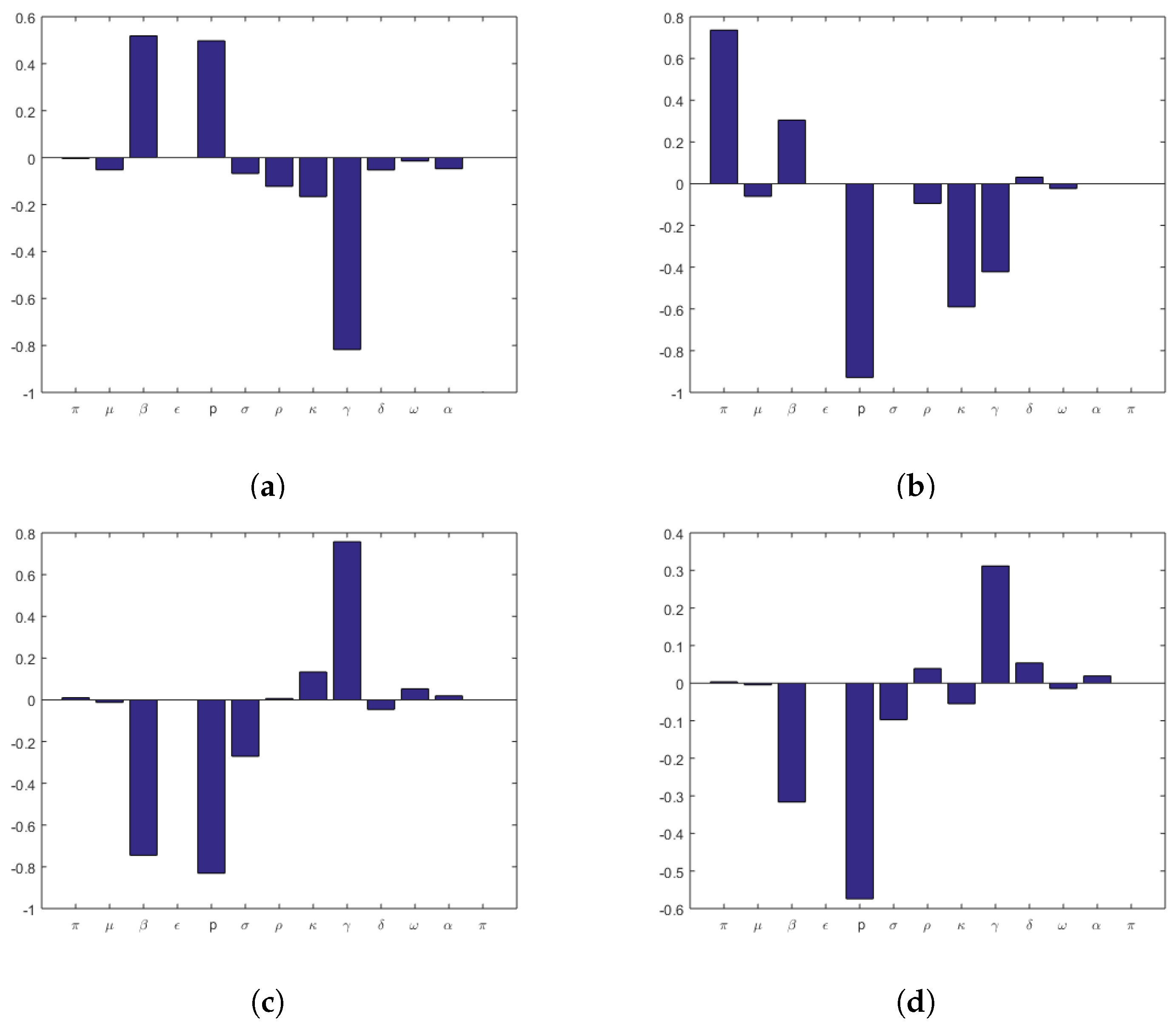
In this study, the parameters with a significant influence on the stigmatised population $I_s$ are shown in Figure 3 for all four waves of COVID-19. Figure 3a shows the PRCC analysis for COVID-19 first wave. Parameters $\beta$, p, and $\gamma$ show PRCC values of more than $0.5$ in the first wave of COVID-19. From Figure 3a, we observe that the most influential LHS parameters for the outcome measure in the $I_s$ are as follows:

• Increasing the effective transmission rate $\beta$, which drives the infection in the total population, and also increases stigmatised infections.
• An increase in the proportion p of stigmatised infections will also increase the stigma in the population
• The parameter $\gamma$ negatively correlates with $I_s,$ meaning the increase in unstigmatisation will decrease the COVID-19 stigmatised population.

On the other hand, in Figure 3b, for the second wave of COVID-19, we observe a strong correlation in parameters $\pi$, p, and $\kappa$. Increasing the recruitment rate $\pi$ will also impact the stigmatised population. The parameters p and $\kappa$ are negatively correlated to $I_s$. In Figure 3c,d, for the third and fourth wave of COVID-19, we observe a strong correlation in parameters $\beta$, p, and $\gamma$.

The p-value of the PRCC shows the significance of the value. A state variable is sensitive to a parameter if the absolute value of the PRCC is more significant than $0.5$ (>0.5 or <−0.5) and the corresponding p-value is lower than $0.05$ [38]. The results showing the p-value for each parameter from the PRCC plots are summarized in

Table 3. Output from PRCC analysis.

		p-Value
Parameters	Wave 1	Wave 2	Wave 3	Wave 4
$\pi$	0.879990	2.401 × 10${}^{-2}$	0.71379	0.910930
$\mu$	0.091592	0.059767	0.72549	0.897160
$\beta$	1.4 × 10${}^{-7}$	4.7 × 10${}^{-2}$	1.6 × 10${}^{-2}$	1.2 × 10${}^{-2}$
$ϵ$	0.960410	0.633470	0.81915	0.975520
p	7.4 × 10${}^{-6}$	0.000000	3.205 × 10${}^{-3}$	1.3 × 10${}^{-9}$
$\sigma$	0.034164	0.779620	2.3 × 10${}^{-2}$	0.0020758
$\rho$	0.0001013	0.002839	0.84352	0.221730
$\kappa$	1.1 × 10${}^{-7}$	4.7 × 10${}^{-9}$	2.4 × 10${}^{-5}$	0.082288
$\gamma$	8.7 × 10${}^{-2}$	2.5 × 10${}^{-4}$	2.1 × 10${}^{-2}$	5.6 × 10${}^{-2}$
$\delta$	0.106480	0.306690	0.13593	0.089534
$\omega$	0.619720	0.454630	0.10030	0.653620
$\alpha$	0.126880	0.633470	0.55529	0.548380

. In this table, essential contributors to uncertainty have their p-values shown in dark bold.

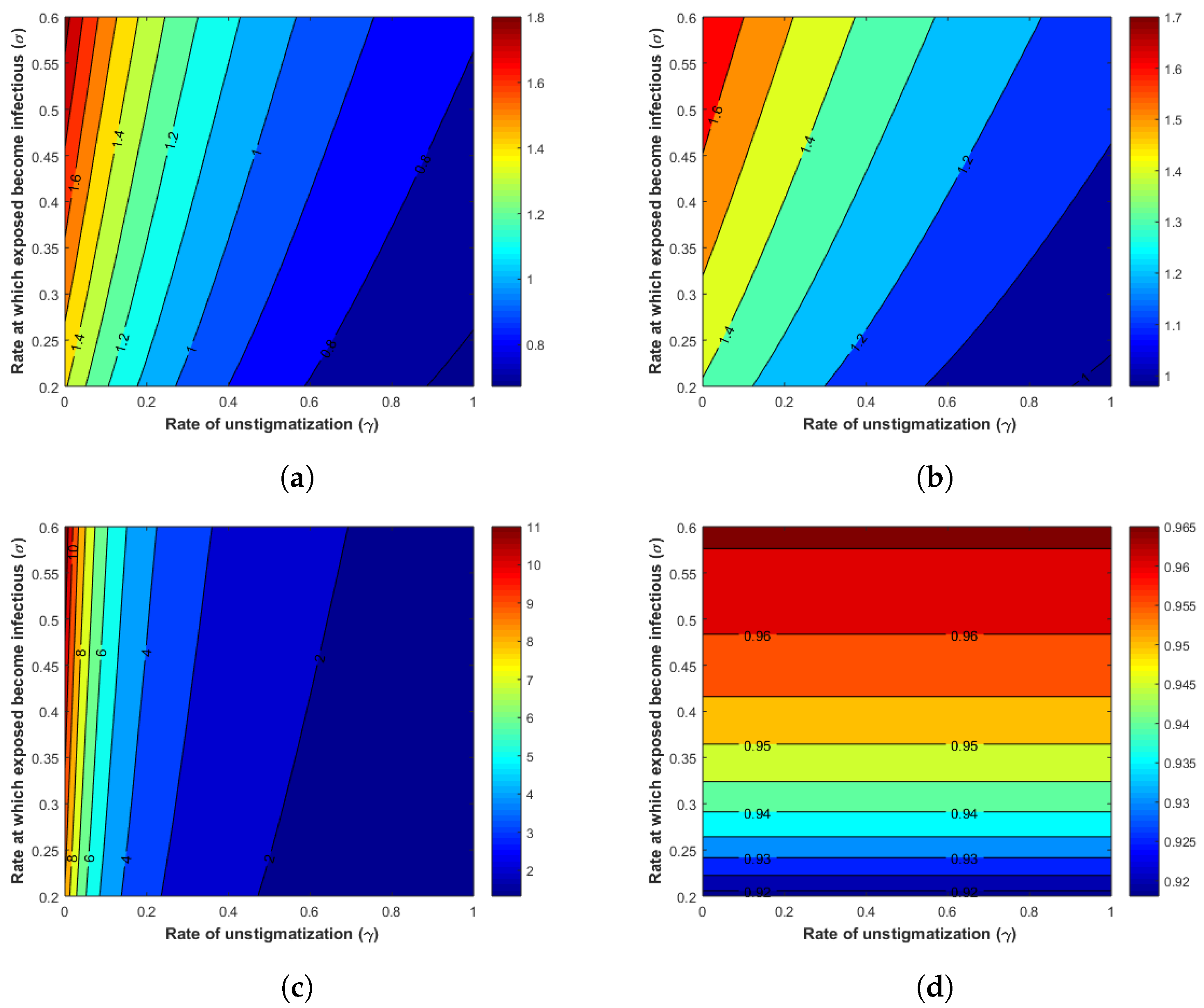
5.3. Effects of Parameters on the $R_0$

We analysed the effects of parameters on $R_0$ using the contour plots in all three COVID-19 waves. We chose two significant parameters, $\sigma$, and $\gamma$, and gave the contour plot as a function of $R_0$. Figure 4 shows that when $\sigma$ increases, $R_0$ also increases, and when $\gamma$ increases, $R_0$ decreases. This implies that new infections are produced when the exposed population becomes infectious, and when stigmatised individuals move to the unstigmatised population, new infections become less in the population.

5.4. Effects of Stigma

To assess and analyse the effects of stigma in COVID-19, we examined four regimes: high stigma, moderate stigma, low stigma, and stigma-free by focusing in the parameters $\gamma$ & p. We define the four categories in terms of parameter values as follows:

i

high stigma $\gamma =0,p=0.49,$

ii

moderate stigma $\gamma =0.4,p=0.49,$

iii

low stigma $\gamma =0.8,p=0.49,$ and

iv

stigma-free $\gamma =0,p=0.$

We varied the impact of stigma using the rate at which stigmatised become non-stigmatised individuals $\gamma$ to assess mild versus high stigma regimes and turned off the proportion p of individuals in E class entering the stigma compartment for the no-stigma case.

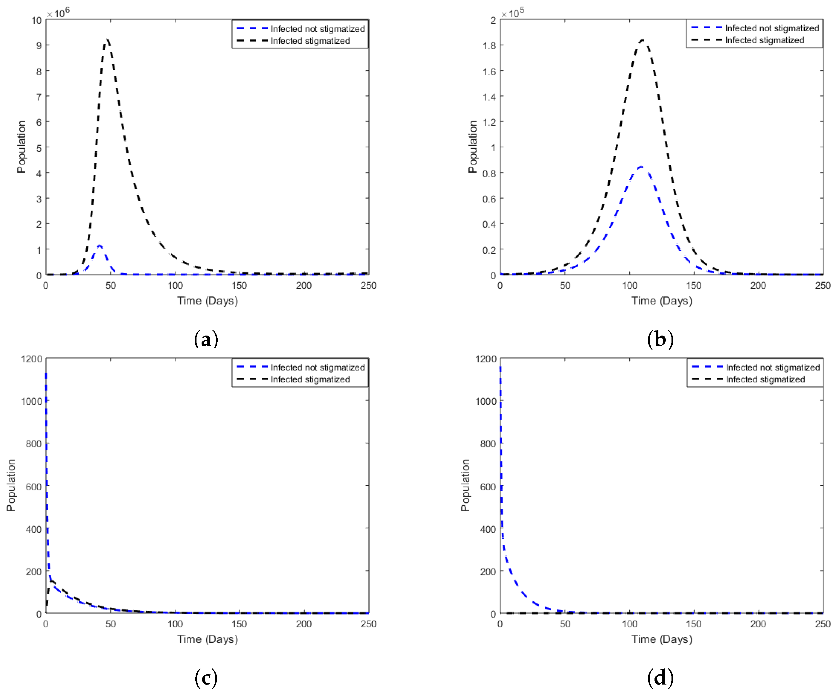
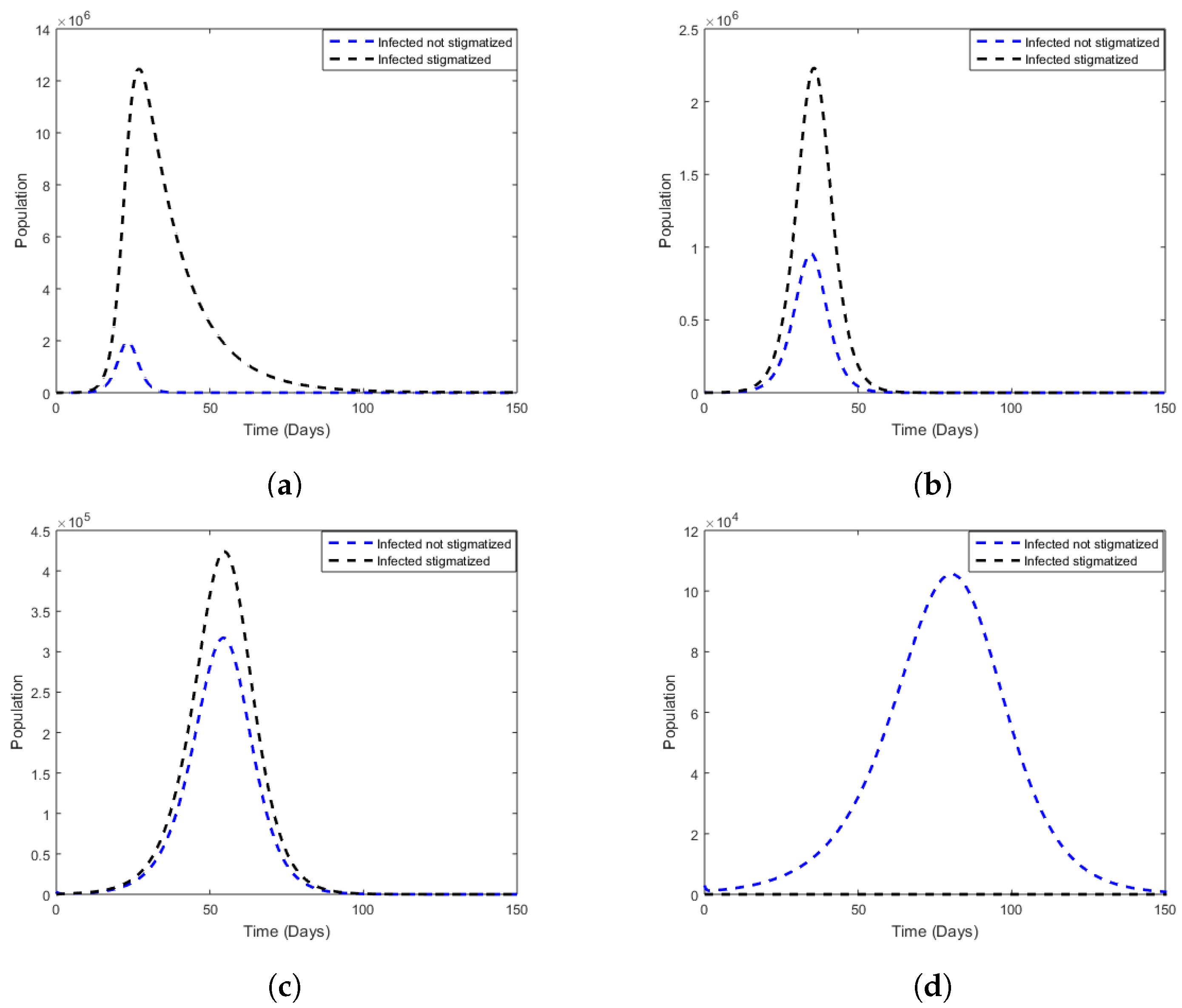
Figure 5a, Figure 6a, Figure 7a and Figure 8a used the parameter values from Table 1, except that we changed the rate at which stigmatised become non-stigmatised to $\gamma =0.1$. This shows a situation where the population has a high stigma. Most of the individuals remain in the stigmatised population for a while. In this case, the number of stigmatised individuals exceeds that of non-stigmatised individuals, sustaining a high level of infected individuals.

Figure 5b, Figure 6b, Figure 7b and Figure 8b show a moderate stigma in the population, where $\gamma =0.4$. These plots indicate a slow progression from stigmatised individuals to a non-stigmatised population.

Figure 5c, Figure 6c, Figure 7c and Figure 8c show a low stigma in the population, where $\gamma =0.8$. These plots indicate that stigmatised individuals move to a non-stigmatised population.

Figure 5d, Figure 6d, Figure 7d and Figure 8d show a case where there is no stigma in the population $(\gamma =0$ and $p=0)$. This indicates that all infected individuals are not stigmatised.

• Wave 1

  Figure 5. Comparison between non-stigmatised and stigmatised populations, varying $\gamma$ for fixed values of p for the cases where there is stigma. (a) High stigma, $\gamma =0$ and $p=0.49$. (b) Moderate stigma, $\gamma =0.4$ and $p=0.49$. (c) Low stigma, $\gamma =0.8$ and $p=0.49$. (d) Stigma-free, $\gamma =0$ and $p=0$.

  Figure 5. Comparison between non-stigmatised and stigmatised populations, varying $\gamma$ for fixed values of p for the cases where there is stigma. (a) High stigma, $\gamma =0$ and $p=0.49$. (b) Moderate stigma, $\gamma =0.4$ and $p=0.49$. (c) Low stigma, $\gamma =0.8$ and $p=0.49$. (d) Stigma-free, $\gamma =0$ and $p=0$.
• Wave 2

  Figure 6. Comparison between non-stigmatised and stigmatised populations, varying $\gamma$ for fixed values of p for the cases where there is stigma. (a) High stigma, $\gamma =0$ and $p=0.49$. (b) Moderate stigma, $\gamma =0.4$ and $p=0.49$. (c) Low stigma, $\gamma =0.8$ and $p=0.49$. (d) Stigma-free, $\gamma =0$ and $p=0$.

  Figure 6. Comparison between non-stigmatised and stigmatised populations, varying $\gamma$ for fixed values of p for the cases where there is stigma. (a) High stigma, $\gamma =0$ and $p=0.49$. (b) Moderate stigma, $\gamma =0.4$ and $p=0.49$. (c) Low stigma, $\gamma =0.8$ and $p=0.49$. (d) Stigma-free, $\gamma =0$ and $p=0$.
• Wave 3

  Figure 7. Comparison between non-stigmatised and stigmatised populations, varying $\gamma$ for fixed values of p for the cases where there is stigma. (a) High stigma, $\gamma =0$ and $p=0.49$. (b) Moderate stigma, $\gamma =0.4$ and $p=0.49$. (c) Low stigma, $\gamma =0.8$ and $p=0.49$. (d) Stigma-free, $\gamma =0$ and $p=0$.

  Figure 7. Comparison between non-stigmatised and stigmatised populations, varying $\gamma$ for fixed values of p for the cases where there is stigma. (a) High stigma, $\gamma =0$ and $p=0.49$. (b) Moderate stigma, $\gamma =0.4$ and $p=0.49$. (c) Low stigma, $\gamma =0.8$ and $p=0.49$. (d) Stigma-free, $\gamma =0$ and $p=0$.
• Wave 4

  Figure 8. Comparison between non-stigmatised and stigmatised populations, varying $\gamma$ for fixed values of p for the cases where there is stigma. (a) High stigma, $\gamma =0$ and $p=0.49$. (b) Moderate stigma, $\gamma =0.4$ and $p=0.49$. (c) Low stigma, $\gamma =0.8$ and $p=0.49$. (d) Stigma-free, $\gamma =0$ and $p=0$.

  Figure 8. Comparison between non-stigmatised and stigmatised populations, varying $\gamma$ for fixed values of p for the cases where there is stigma. (a) High stigma, $\gamma =0$ and $p=0.49$. (b) Moderate stigma, $\gamma =0.4$ and $p=0.49$. (c) Low stigma, $\gamma =0.8$ and $p=0.49$. (d) Stigma-free, $\gamma =0$ and $p=0$.

5.5. Cumulative Cases

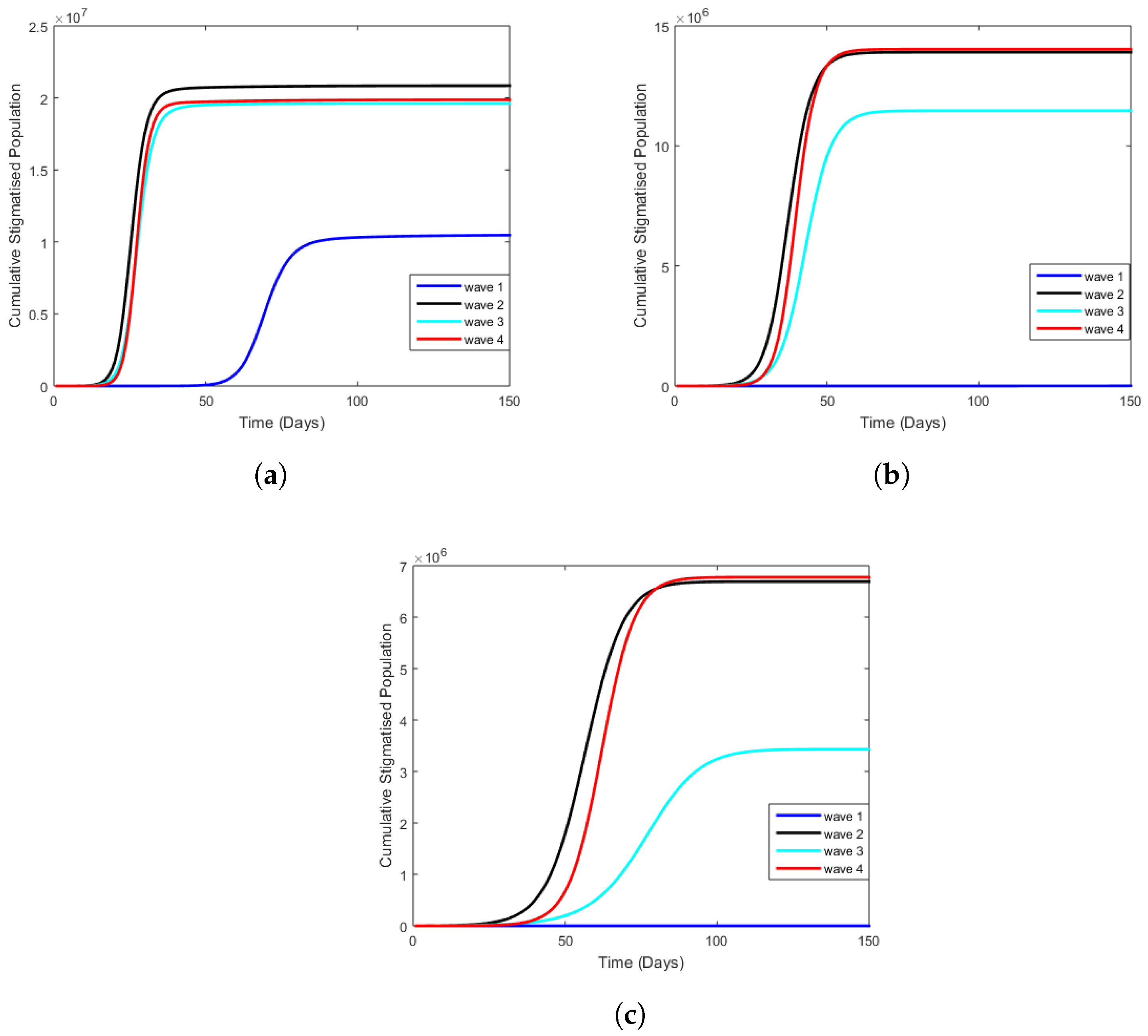
In the figures below, we analyze cumulative cases for each wave and per regime using the same stigma regimes, parameters, and initial conditions as in previous figures. In Figure 9a, we observe that the first wave of COVID-19 had the lowest number of stigmatised individuals when the stigma was high. In contrast, the second wave had the highest number of cumulative cases. The reason could be that the second wave was associated with a higher incidence of COVID-19, more rapid hospital admissions, and increased in-hospital mortality [39]. Figure 9b,c show that when stigma is moderate and low, there are no stigmatised individuals during the first wave, and the fourth wave has higher stigmatised individuals.

5.6. Estimated Reproduction Number

Table 4. The estimated basic reproduction number for COVID-19 waves in South Africa.

Wave 1
	High	Moderate	Low	Stigma-free
$R_1$	7.2258	0.8804	0.4688	0
$R_2$	3.8768	0.8249	0.6270	0.7873
$R_0$	11.1025	1.7054	1.0957	0.7873
Wave 2
	High	Moderate	Low	Stigma-free
$R_1$	9.4060	1.5035	0.8170	0
$R_2$	5.2237	1.3468	1.0100	1.1944
$R_0$	14.6296	2.8502	1.8270	1.1944
Wave 3
	High	Moderate	Low	Stigma-free
$R_1$	7.4634	1.4457	0.8004	0
$R_2$	4.7434	1.4289	1.0734	1.2404
$R_0$	12.2069	2.8746	1.8738	1.2404
Wave 4
	High	Moderate	Low	Stigma-free
$R_1$	$12.5406$	$2.0045$	$1.08934$	0
$R_2$	$4.2248$	$1.0892$	$0.8169$	$0.9660$
$R_0$	$16.7655$	$3.0937$	$1.9062$	$0.9660$

shows the estimated reproduction numbers for each COVID-19 wave per stigma regime (high, moderate, low stigma, and stigma-free). The estimates in $R_1$ represent the number of new COVID-19 infections generated by the stigmatised infectious population, and $R_2$ represents the number of new COVID-19 infections provoked by the non-stigmatised contagious population. $R_0$ gives the total number of new infections caused by both infectious populations. Here, we observe that when stigma is high in the community, the basic reproduction number is also high, and the contribution from the stigmatised to $R_0$ is higher than that from the unstigmatised. Additionally, when stigma is moderate and low, $R_0$ is still greater than one, and the stigmatised population’s contribution is higher than the unstigmatised population. When there is no stigma in the community, $R_1=0$ since $R_1$ represents new infections generated by stigmatised individuals.

5.7. Contribution of Stigma

This section shows how stigma is contributed to the population based on stigma regimes.

Table 5. The area between two curves for COVID-19 waves.

	High	Moderate	Low
Wave 1	2.9844 × ${10}^8$	3.9118 × 10${}^6$	2.5920 × 10${}^4$
Wave 2	3.6056 × ${10}^8$	2.7355 × 10${}^7$	2.9714 × 10${}^6$
Wave 3	2.7919 × ${10}^8$	2.2650 × 10${}^7$	2.1844 × 10${}^6$
Wave 4	4.3391 × ${10}^8$	4.3665 × 10${}^7$	8.2119 × 10${}^6$

shows the calculated area between stigmatised and non-stigmatised populations. The area is also significant when stigma is in a high state regime.

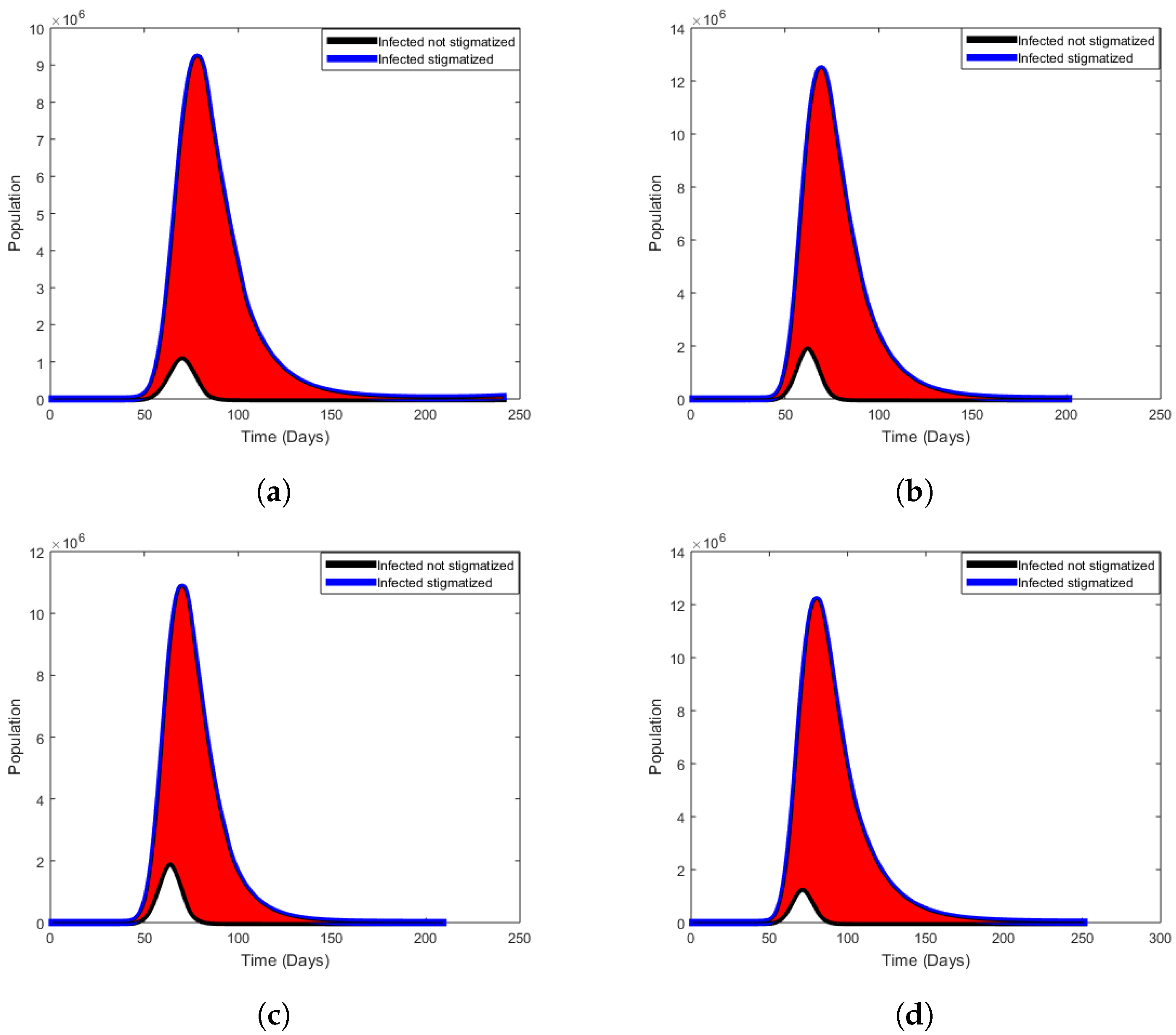
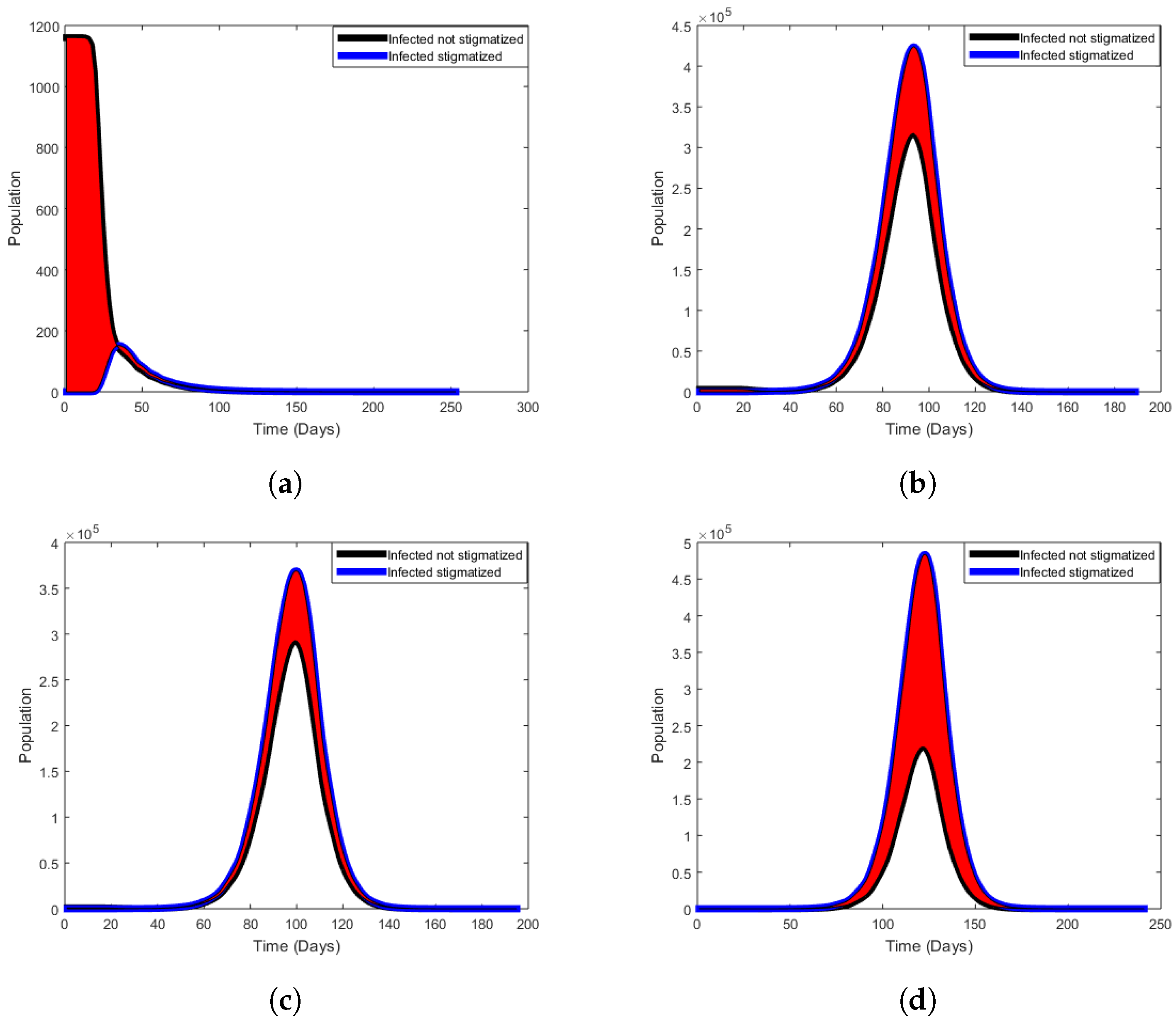
Figure 10, Figure 11 and Figure 12 show the contribution of stigma in the population. The area shaded with red indicates how COVID-19 stigma affects the people in the community per stigma regimes.

5.7.1. High Stigma Regime

Figure 10 shows that high stigma in all four waves increases the stigmatised infectious population, $I_s$, and decreases the non-stigmatised infectious population, $I_n$. This results from more people concealing their statuses to avoid being discriminated against by the community.

5.7.2. Moderate Stigma Regime

Figure 11 shows that even though stigma is moderate, there is an increase in the stigmatised infectious population, $I_s$, and a decrease in the non-stigmatised infectious population, $I_n$.

5.7.3. Low Stigma Regime

Figure 12 shows that low stigma in all four waves decreases the stigmatised infectious population, $I_s$, and increases the non-stigmatised infectious population, $I_n$. More people are disclosing their COVID-19 status, and less stigma exists in the population.

6. Conclusions

Our motivation in undertaking the work presented here was to understand the potential impact of stigma on the transmission dynamics of COVID-19 in South Africa. We classified the stigma as either low, moderate, or high. We presented a deterministic model to assess the impact of stigma on the transmission dynamics of COVID-19 in South Africa. The model considers the susceptible, exposed, non-stigmatised, stigmatised, hospitalized, and recovered humans. The model reproduction number $R_0$ was determined by using the next-generation matrix method. Mathematical analysis for the model showed that the equilibrium points are locally asymptotically stable if $R_0$ is more than one and if $R_0$ is less than one is unstable. The Lyapunov functions were used in the establishment of global stability for both disease-free and endemic equilibria. Furthermore, the sensitivity analysis of the model equations was performed, p-values for parameters were obtained, and numerical simulations based on the highly sensitive model parameters on $R_0,$ as shown in Figure 3. We also analysed the effects of parameters on $R_0$ using the contour plots in all four COVID-19 waves. We thus see that low, moderate, or high stigma plays a significant role in sustaining COVID-19 in the population. In Table 4, our analysis demonstrated that $R_0$ tends to range from $0.7489$ to $14.6296$ depending on stigma regimes.

The COVID-19 pandemic has continued to spread, causing many deaths, and stigma is an essential factor in the spread of COVID-19. In practice, COVID-19 eradication strategies should focus on reducing COVID-19-related stigma through educating individuals about the disease. Our model has some limitations, which should be acknowledged. We combined ‘disclosure’ and ‘stigma’, whereas, in practice, the social phenomenon of COVID-19-related stigma is more complex. We represent stigma by way of parameter choices, which simplifies this case. Thus, further refinement for this study would be to model the stigma parameters as randomly time-varying functions. Aspects of delays in the stigmatised accessing help can also be modelled by delay differential equations.

References

- SA Coronavirus. About COVID-19 (Coronavirus). Available online: https://sacoronavirus.co.za/information-about-the-virus-2/ (accessed on 27 February 2021).
- Sotgiu, G.; Dobler, C.C. Social stigma in the time of Coronavirus. Eur. Respir. J. 2020, 56, 2002461. [Google Scholar] [CrossRef]
- Donthu, N.; Gustafsson, A. Effects of COVID-19 on business and research. J. Bus. Res. 2020, 117, 284–289. [Google Scholar] [CrossRef] [PubMed]
- Chu, D.K.; Akl, E.A.; Duda, S.; Solo, K.; Yaacoub, S.; Schünemann, H.J. Physical distancing, face masks, and eye protection to prevent person-to-person transmission of SARS-CoV-2 and COVID-19: A systematic review and meta-analysis. Lancet 2020, 395, 1973–1987. [Google Scholar] [CrossRef]
- MacIntyre, C.R.; Wang, Q. Physical distancing, face masks, and eye protection for prevention of COVID-19. Lancet 2020, 395, 1972. [Google Scholar] [CrossRef]
- Goffman, E. Stigma: Notes on the Management of Spoiled Identity; Simon and Schuster: New York, NY, USA, 2009; p. 1. Available online: https://archive.org/details/stigmanotesonman00goff_0/page/1/mode/2up (accessed on 1 March 2021).
- Pescosolido, B.A. The public stigma of mental illness: What do we think; what do we know; what can we prove? J. Health Soc. Behav. 2013, 54, 1–21. [Google Scholar] [CrossRef]
- Caddell, J. What Is Stigma. Social Psychology. 2020. Available online: https://www.verywellmind.com/mental-illness-and-stigma-2337677 (accessed on 1 March 2021).
- Campbell, C.; Deacon, H. Unraveling the contexts of stigma: From internalisation to resistance to change. J. Community Appl. Soc. Psychol. 2006, 16, 411–417. [Google Scholar] [CrossRef]
- Gray, A.J. Stigma in psychiatric. J. R. Soc. Med. 2002, 95, 72–76. [Google Scholar] [CrossRef] [PubMed]
- Schnyder, N.; Panczak, R.; Groth, N.; Schultze-Lutter, F. Association between mental health-related stigma and active help-seeking: Systematic review and meta-analysis. Br. J. Psychiatry 2017, 210, 261–268. [Google Scholar] [CrossRef] [PubMed]
- Centers for Disease Control and Prevention. Reducing Stigma. 2020. Available online: https://www.cdc.gov/coronavirus/2019-ncov/daily-life-coping/reducing-stigma.html#:~:text=Stigma%20is%20associated%20with%20a,others%20to%20spread%20COVID%2D19 (accessed on 18 September 2021).
- World Health Organization. Social Stigma Associated with COVID-19; World Health Organization: Geneva, Switzerland, 2020. [Google Scholar]
- Sintunavarat, W.; Turab, A. Mathematical analysis of an extended SEIR model of COVID-19 using the ABC-fractional operator. Math. Comput. Simul. 2022, 198, 65–84. [Google Scholar] [CrossRef]
- Rezapour, S.; Souid, M.S.; Bouazza, Z.; Hussain, A.; Etemad, S. On the fractional variable order thermostat model: Existence theory on cones via wiece-wise constant functions. J. Funct. Spaces 2022, 2022, 8053620. [Google Scholar] [CrossRef]
- Rezapour, S.; Abbas, M.I.; Etemad, S.; Dien, N.M. On a multi-point p-Laplacian fractional differential equation with generalized fractional derivatives. Math. Methods Appl. Sci. 2022, 1–18. [Google Scholar] [CrossRef]
- Mukandavire, Z.; Nyabadza, F.; Malunguza, N.J.; Cuadros, D.F.; Shiri, T.; Musuka, G. Quantifying early COVID-19 outbreak transmission in South Africa and exploring vaccine efficacy scenarios. PLoS ONE 2020, 15, e0236003. [Google Scholar] [CrossRef]
- Nyabadza, F.; Chirove, F.; Chukwu, W.C.; Visaya, M.V. Modelling the potential impact of social distancing on the COVID-19 epidemic in South Africa. Comput. Math. Methods Med. 2020, 2020, 5379278. [Google Scholar] [CrossRef] [PubMed]
- Gatyeni, S.P.; Chukwu, C.W.; Chirove, F.; Fatmawati; Nyabadza, F. Application of Optimal Control to the Dynamics of COVID-19 Disease in South Africa. Sci. J. 2022, 16, e01268. [Google Scholar] [CrossRef]
- Mosher, S.G.; Costris-Vas, C.; Smith, R. Modelling the Effects of Stigma on Leprosy; Springer Nature: Singapore, 2020; Available online: https://link.springer.com/chapter/10.1007%2F978-981-15-0422-8_5 (accessed on 5 April 2021).
- Lengiteng’i, L.; Kajunguri, D.; Nkansah-Gyekye, Y. Modeling the effect of stress and stigma on the transmission and control of Tuberculosis infection. Am. Sci. Res. J. Eng. Technol. Sci. 2018, 24, 26–50. [Google Scholar]
- Accord. Stigma and Discrimination: Consequences of the Fear of COVID-19. 2020. Available online: https://www.accord.org.za/analysis/stigma-and-discrimination-consequences-of-the-fear-of-covid-19/ (accessed on 8 December 2021).
- Diekmann, O.; Heesterbeek, J.A.P.; Metz, J.A.J. On the definition and the computation of the basic reproduction ratio R0 in models for infectious diseases in heterogeneous populations. Math. Biol. 1990, 28, 365–382. [Google Scholar] [CrossRef] [PubMed]
- van den Driessche, P.; Watmough, J. Reproduction numbers and sub-threshold endemic equilibria for compartmental models of disease transmission. Math. Biol. 2002, 180, 29–48. [Google Scholar] [CrossRef]
- LaSalle, J.; Lefschetz, S.; Alverson, R.C. Stability by Liapunov’s Direct Method with Applications; Academic Press: New York, NY, USA, 1962. [Google Scholar]
- LaSalle, J. The Stability of Dynamical System; SIAM: Philadelphia, PA, USA, 1976. [Google Scholar]
- Guo, H.; Li, M.Y. Global stability of tuberculosis model with immigration and treatment. Can. Appl. Math. Quaterly 2006, 14, 185–197. [Google Scholar]
- Statistics. March 2020. Available online: https://www.airports.co.za/news/statistics (accessed on 30 November 2021.).
- Stats SA. COVID-19 Epidemic Reduces Life Expectancy in 2021. Available online: http://www.statssa.gov.za/?p=14519 (accessed on 30 November 2021).
- Ki, M. Task force for 2019-nCoV. Epidemiologic characteristics off early cases with 2019 novel coronavirus (2019-nCoV) disease in Korea. Epidemiol. Health 2020, 42, e2020007. [Google Scholar] [CrossRef]
- Ullah, S.; Khan, M.A. Modeling the impact of non-pharmaceutical interventions on the dynamics of novel coronavirus with optimal control analysis with a case study. Chaos Solitons Fractals 2020, 139, 110075. [Google Scholar] [CrossRef]
- Li, Q.; Guan, X.; Wu, P.; Wang, X.; Zhou, L.; Tong, Y.; Ren, R.; Leung, K.S.M.; Lau, E.H.Y.; Wong, J.Y.; et al. Early transmission dynamics in Wuhan, China, of novel coronavirus-infected pneumonia. N. Engl. J. Med. 2020, 382, 1199–1207. [Google Scholar] [CrossRef] [PubMed]
- Daily Maverick. Research Data Indicates Deaths from COVID-19 Are More Than Double the Official Count in South Africa. Available online: https://www.dailymaverick.co.za/article/2021-08-12-research-data-indicates-deaths-from-covid-19-are-more-than-double-the-official-count-in-south-africa/ (accessed on 2 December 2021).
- Saltelli, A.; Ratto, M.; Andries, T.; Campolongo, F.; Cariboni, J.; Gatelli, D.; Saisana, M.; Tarantola, S. Global Sensitivity Analysis: The Primer; John Wiley and Sons: Hoboken, NJ, USA, 2008. [Google Scholar]
- Blower, S.M.; Hartel, D.; Dowlatabadi, H.; Anderson, R.M.; May, R.M. Drugs, sex and HIV: A mathematical model for New York city. Philos. Trans. Biol. Sci. 1991, 331, 171–187. [Google Scholar]
- Taylor, R. Interpretation of the Correlation Coefficient: A Basic Review. J. Diagn. Med. Sonogr. 1990, 1, 35–39. [Google Scholar] [CrossRef]
- Gomero, B. Latin Hypercube Sampling and Partial Rank Correlation Coefficient Analysis Applied to an Optimal Control Problem, University of Tennessee. 2012. Available online: https://trace.tennessee.edu/utk_gradthes/1278 (accessed on 20 May 2022).
- Pennington, H.M. Applications of Latin Hypercube Sampling Scheme and Partial Rank Correlation Coefficient Analysis to Mathematical Models on Wound Healing, Honors College Capstone Experience/Thesis Projects. Paper 581. 2015. Available online: http://digitalcommons.wku.edu/stu_hon_theses/581 (accessed on 20 May 2022).
- Jassat, W.; Mudara, C.; Ozougwu, L.; Tempia, S.; Blumberg, L.; Davies, M.; Pillay, Y.; Carter, T.; Morewane, R.; Wolmarans, M.; et al. DATCOV author group, Difference in mortality among individuals admitted to hospital with COVID-19 during the first and second waves in South Africa: A cohort study. Lancet Glob. Health 2021, 9, e1216-25. [Google Scholar] [CrossRef]
Figure 1.
A model flow diagram for COVID-19 infection dynamics. The diagram shows the flow of individuals from one compartment to the other as their infection status with respect to the disease changes.
Figure 2.
Model fit to data for COVID-19 waves in South Africa. (a) Wave 1 model fit. (b) Wave 2 model fit. (c) Wave 3 model fit. (d) Wave 4 model fit.
Figure 3.
PRCCs for during the COVID-19 waves. (a) Wave 1. (b) Wave 2. (c) Wave 3. (d) Wave 4.
Figure 4.
Contour plots of . (a) Wave 1. (b) Wave 2. (c) Wave 3. (d) Wave 4.
Figure 9.
Comparison between cumulative stigmatised populations. (a) High stigma cumulative cases. (b) Moderate stigma cumulative cases. (c) Low stigma cumulative cases.
Figure 10.
High regime state. (a) Wave 1. (b) Wave 2. (c) Wave 3. (d) Wave 4.
Figure 11.
Moderate regime state. (a) Wave 1. (b) Wave 2. (c) Wave 3. (d) Wave 4.
Figure 12.
Low regime state. (a) Wave 1. (b) Wave 2. (c) Wave 3. (d) Wave 4.