1. Introduction
Ambient air pollution places a large burden on human health and welfare, as it is estimated to cause millions of premature deaths worldwide [
1]. More specifically, the years of life lost from ambient particulate matter pollution causes enormous social and economic stress [
1]. Recently, the concentrations of various primary and secondary air pollutants in Europe have shown a downward trend [
2]. Nevertheless, air pollution is, according to the European Environmental Agency (EEA), still “the biggest environmental health risk” in Europe [
2]. In urban areas, air pollution is caused by local road traffic, industry, and household emissions, but it also comes from the advection of pollutants from upwind sources.
We have been studying the complex interplay between emissions, atmospheric transformation processes (e.g., heterogeneous reactions) and local transport and mesoscale meteorology for the city of Münster, Germany, since 2004 [
3,
4,
5,
6,
7,
8,
9,
10,
11]. Besides the transport patterns themselves [
12,
13], we have been primarily interested in the dynamics of particulate matter and of nitrogen compounds. Motorized street traffic is a major source of nitrogen oxides (NO
x) and aerosol particles. We found that the city is a net emission source of fine particles (aerodynamic diameters below about 200 nm), while it is a sink for larger particles that are advected from upwind sources [
6,
14,
15]. Reduced nitrogen emissions from agricultural sources interact with aerosol particles both upwind and within the city and, thus, impact the composition and size distribution of aerosol particles [
4,
5,
6,
9]. Generally, the concentrations of primary air pollutants are both higher in winter than in summer and during the night than in the daytime [
16]. This implies that the stability of the boundary layer should be an important driver of air pollution levels. However, statistical analysis on short-term datasets could not confirm a strong impact of stability on air pollutant concentrations in Münster; instead, the impact of temperature, humidity, and wind was much stronger [
5,
10].
As the interplay between meteorology and air pollution is complex, this represents a challenging field in environmental education at the undergraduate level. Within the relatively short time frame of an undergraduate education, students must gain a comprehensive understanding of the essential features of a multidimensional space. Once the basis of the theoretical principles has been laid, students can make the most efficient learning progress with hands-on, self-driven research. In one such promising project, students revisited the studies mentioned above on how traffic and meteorology affect urban, airborne particle concentrations in Münster. Yet, the students employed a newer approach in order to incorporate novel techniques and to allow for more advanced experimental designs than those used just a few years earlier.
In this project, a voluntary group of six undergraduate students (bachelor’s level) in environmental sciences performed a study in which a cargo bicycle platform was used to map the particle concentrations along urban routes. The cargo bicycle was largely identical to the bicycle that had been used not long before by [
11,
17], so the focus of the students’ project was on study design, realization of data acquisition, and scientific analysis. Shortly after termination of this initial project in November 2019, the COVID-19 pandemic led to a strict lockdown in Germany (see
Section 2 for details), and one of the students decided to make additional bicycle rides during conditions of very low traffic intensity. In November 2020, a different group of students (10 participants) performed a follow-up study using an identical experimental approach in order to complement the existing dataset with data from a less stringent lockdown period. Finally, another student made further measurement rides in March and April 2021 to collect data under “normal” circumstances, since at this time most of the pandemic restrictions had been lifted.
Overall, these data consist of measurements from 40 rides with the instrumented cargo bicycle that cover a time period of about 1.5 years (October 2019–April 2021) from before the pandemic lockdowns in Germany through to the time in which they were lifted. Meteorological and particle concentration measurements were made with rather high temporal resolution (1 Hz) along two routes (high traffic, low traffic) during each ride. However, the study design was not optimized in terms of covering various meteorological conditions and seasons of the year. Yet, because the measurements covered situations with both very high and very low urban traffic intensities, the patchwork database should be large enough to address the impact of traffic and meteorology on urban aerosol particle concentrations via a scientific approach. One of the focal points of the study was to separate the dynamics of particle number concentrations (PN) on the one hand and particle mass concentrations on the other. While the particle mass concentrations (PM10, PM2.5) are regulated by European threshold limits, particle number concentrations are believed to be of high toxicological relevance for humans [
18]. The concentration of ultrafine particles, which typically dominate the PN concentration, are closely related to emissions from motorized vehicles at urban traffic sites.
This analysis pursues the hypotheses (i) that motorized vehicle road traffic is a main driver of the aerosol particle concentrations at the urban street level, (ii) that this impact is expressed through a clearly higher level of particle concentrations on a route with high traffic intensity as compared to a route with low traffic intensity, (iii) that this impact also appears through a response of the general urban particle concentration levels as a function of traffic intensity, some of which are governed by enforced lockdowns, (iv) that the particle number concentrations (PN) respond to traffic more strongly than do the particle mass concentrations (PM1, PM2.5, PM10), and, finally, (v) that boundary layer exchange conditions, expressed through the stability of the boundary layer and wind speed, also play important roles in driving particle concentrations.
We will present the cargo bicycle, its instrumentation, and the measurement routes in
Section 2. In
Section 3, the lockdown periods are characterized and the results of the mobile measurements are shown. Focus is on the response of PN and PM10 to the traffic intensity. One ride is presented in detail, while the results of the other 39 rides are presented in condensed form: medians and interquartile ranges are shown as well as the results of a relative importance analysis.
Section 4 discusses the high variability of data along the traveled routes and the mixed response of PN and PM10 to traffic, date, and meteorological conditions. In the conclusions in
Section 5, the special features of this student-led study are summarized, the initial hypotheses are tested, and an outlook for further analyses and experiments is provided.
2. Materials and Methods
Münster is a city of about 312,000 inhabitants [
19] in western to north-western Germany. It lies in rather flat terrain and has a somewhat circular layout around the city center. It hosts only a few small to medium-sized industries while containing many green spaces. It is one of the most bicycle-friendly cities in Germany, which is expressed through many designated cycle paths, specifically a 4.4 km long bicycle and pedestrian path around the city center that follows the track of the former medieval city wall. This “Promenade” is the “low-traffic route” described below.
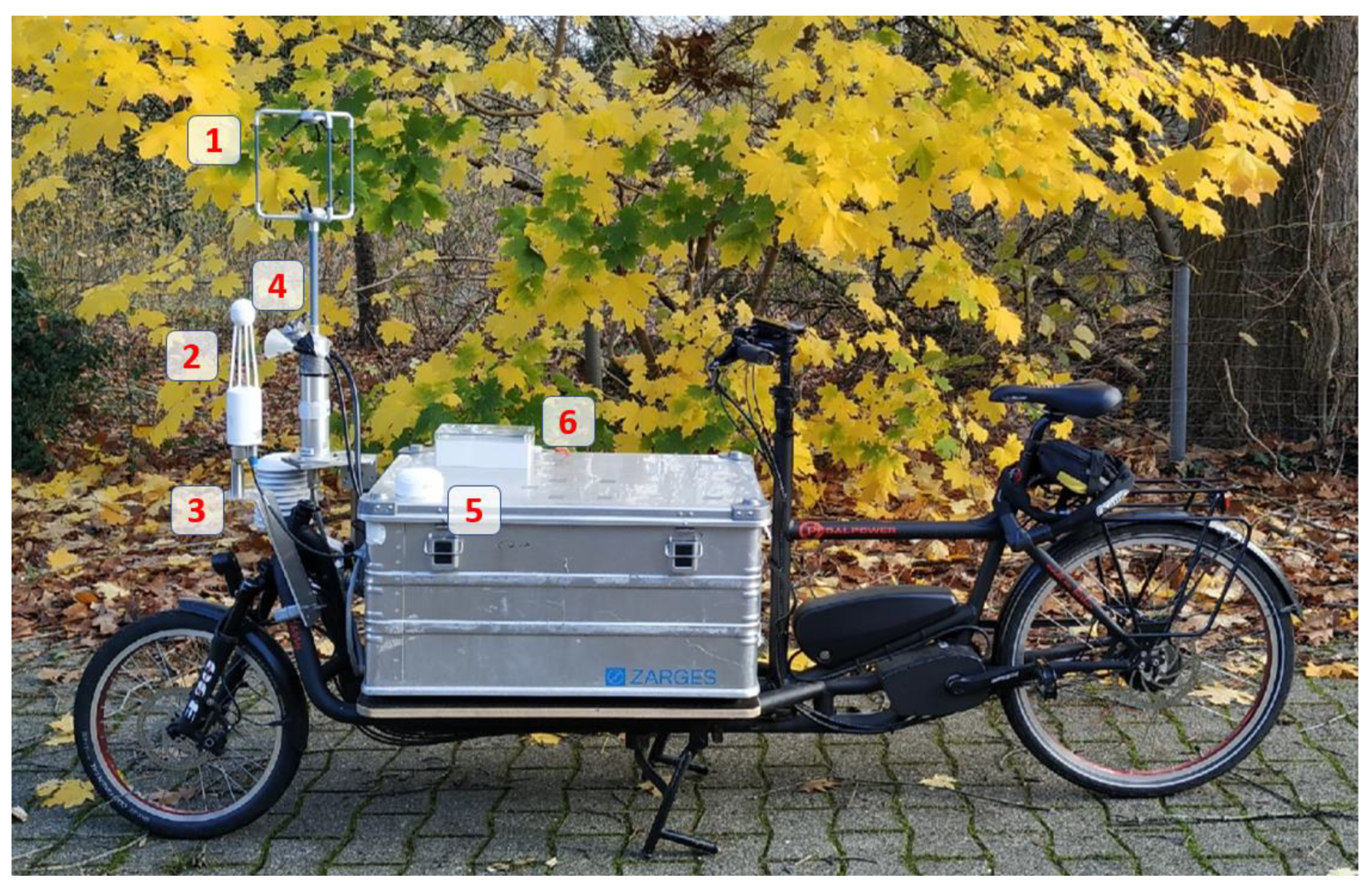
An instrumented cargo bicycle (
Figure 1) was employed to conduct meteorological and air chemistry measurements while cruising along predefined routes in town. The bicycle was equipped as described in [
11], such that its position was measured with a GPS receiver (type 19x HVS, Garmin Ltd., Olathe, KS, USA), the total aerosol particle number concentration PN with a condensation particle counter (CPC, type 3025A, TSI Inc., Shoreview, MN, USA), and the aerosol particle size spectrum with an optical particle spectrometer (OPS, type 3330, TSI Inc., Shoreview, MN, USA). The CPC had an upper detection limit of 53,000 cm
−3 for PN. The OPS measured the particle spectrum in 16 size classes, while only the data for PM1, PM2.5, and PM10 (mass concentrations for aerosol particles with diameters below 1.0, 2.5, and 10 µm, respectively, in µg m
−3) were used for further analysis. The OPS was manufacturer-calibrated before the onset of the experiments. The sample inlet funnels for CPC and OPC were mounted on the front of the bicycle at 1.1 m above street level and facing forward. Data collection was carried out at a 1 Hz time resolution. In addition, further instruments were mounted to measure wind (ultrasonic anemometer in combination with a compass), temperature, humidity, and the concentration of CO
2. These datasets were, however, not analyzed.
A total of 40 rides were made between October 2019 and April 2021. During each ride, two clockwise laps around city center were made while data were collected. The first lap followed the “high-traffic route” along busy roads, in which the route passes by the main gate of the main train station with the largest public bus stop in the city, goes through a two-lane roundabout with six exits, and finally returns to the start-and-stop position, which also was the junction position between the two laps. The high-traffic route was about 4.6 km long, and the average cruising time was 22 min. The second lap followed the “low-traffic route,” which went along the Promenade (described above). This route consists of an avenue with two lanes of large trees (predominantly Tilia cordata) on both sides and has no motorized traffic, yet it intersects several arterial roads with motorized traffic. This low-traffic route was about 4.4 km long, and the average cruising time was 18 min.
Further data on the general meteorology and air pollution conditions were retrieved from the University of Münster’s meteorological station (51.96930 N, 7.59588 E), located about 2 km to the WNW of the city center, from the two urban air pollution monitoring sites VMS2 (51.95328 N, 7.61938 E) and MSGE (51.93654 N, 7.61158 E) of the State Agency for Nature, Environment and Consumer Protection (LANUV), as retrieved from their homepage [
20], and from the closest radiosonde launch site Essen (EDZE, 51.40 N, 6.97 E) of the German Weather Service (DWD), as retrieved from the University of Wyoming’s homepage [
21]. The latter data were utilized to determine the stability of the atmospheric boundary layer from the gradient of the potential temperature within heights of up to about 100 m above ground.
The traffic intensity was measured at intersections containing “modern” traffic lights within the city. Data were provided by the municipality of Münster. Sensors at the intersections count every vehicle and aggregate these counts for each hour. These counts lead to absolute values which are only comparable for the purposes of this study, because they refer to an arbitrary number of intersections. We used all available data to analyze the city’s traffic intensity over the entire study period on the basis of daily averages, while we used the traffic counts of 23 intersections next to the bicycle routes and during riding times to compare these specific time periods with each other. We employed a “relative importance” (relaimpo) statistical model to quantify the (statistical) impact of drivers on the measured particle concentrations during individual laps. The linear model by [
22,
23] applies to explanatory variables that are correlated with each other, which we expect to be the case in our real-world datasets. We modeled the relative importance of 20 drivers representing the traffic intensity, route (high traffic vs. low traffic), season, day of the week, and meteorological and air pollution conditions in Münster during the individual rides. Target parameters were the 10th percentiles, 50th percentiles (medians), and the 90th percentiles as well as the interquartile ranges (25th and 75th percentiles) of the PN, PM1, PM2.5, and PM10 concentrations during each lap (route).
Unpaired Mann–Whitney U tests were used to test the differences between concentration datasets between routes because the data were not normally distributed and were not paired. Brantley et al. [
24] recommended this approach for analyzing data from mobile measurements because it is less prone to outliers and because it avoids bias in near-spatial trends. Analyses to test the differences between paired datasets (e.g., medians of high-traffic route data vs. medians of low-traffic route data) were performed with the Wilcoxon test. The level of confidence for statements of significance is always 0.95.
3. Results
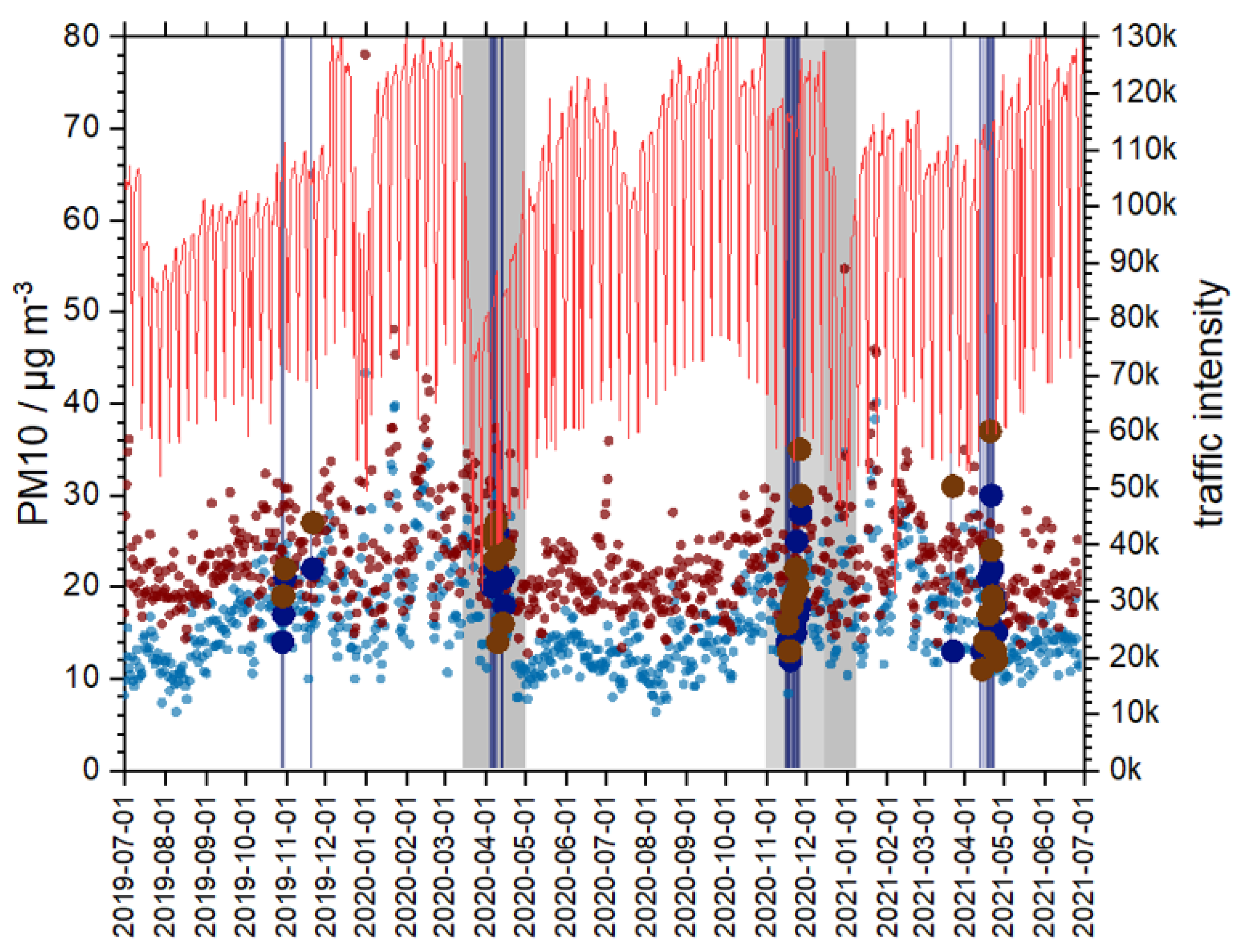
Figure 2 embeds the study period into a larger time frame. Bicycle measurement days are indicated by vertical blue lines. The traffic intensity (red line) is a good indicator for the activity of the city’s commercial and private sectors and of the impact of the German lockdown periods. Note the well-pronounced weekly cycle of the traffic intensity and its response to school holidays (e.g., from 13 July 2019 through 27 August 2019) and to school and business holidays during the Christmas and New Year period 2019/2020. The highest average PM10 concentration of 78 µg m
−3, representing the average of the New Year’s days of the past five years, occurred on 1 January 2020 at the VMS2 station and reflects the fireworks activity in town. The first general lockdown as a response to the COVID-19 pandemic was announced for the period from 23 March 2020 through 19 April 2020 [
25]. Contact restrictions were enforced; schools, restaurants, and non-essential shops were closed; people were strongly encouraged to work from home. This led to a drastic decrease in road traffic, as evident in
Figure 2, yet road traffic steadily increased right after the lockdown started. Good Friday 2020, a national holiday, was among the days with the lowest traffic intensity for the entire period, and it was the day with the lowest traffic intensity among the measurement days (ride 9). More days of low traffic intensity followed during the Easter holiday weekend. A total of nine rides were made during this lockdown period in spring 2020. For days directly after this first lockdown, the traffic only slowly recovered to its normal intensity because people acted carefully and reduced their general mobility amid the ongoing pandemic.
After the summer season of 2020, in which hardly any restrictions and containment measures were in place, the pandemic picked up again. This led to public restrictions being introduced again, this time in a stepwise fashion, starting on 2 November 2020. This period, lasting until 15 December 2020, is referred to here as “lockdown light”. During this period, which is hardly identifiable in the general traffic intensity data (
Figure 2), sixteen bicycle measurement rides were conducted. Later on, from 16 December 2020 through 10 January 2021, a second nationwide lockdown period was put in place over the Christmas and New Year holiday season 2020/2021. No bicycle measurements were made then (
Figure 2). Another eleven rides were made in March and April 2021. Numerous studies have shown that the COVID-19 containment measures led to air quality improvements in urban areas in Europe [
26,
27,
28,
29,
30,
31], Asia [
32,
33,
34,
35,
36,
37,
38], North and South America [
39,
40,
41], and virtually all other regions, including Oceania and Africa [
42]. Studies identified decreases in air pollutants’ concentrations of up to ~60%, where decreases were stronger for NO
x than for PM and stronger for PM2.5 than for PM10. In Germany, urban NO
x concentrations were ~30% lower during the first lockdown period than in the respective time periods of the preceding years [
43]. Besides the lockdowns themselves, the generally decreasing trend of NO
x emissions led to lower concentrations in 2020 than in previous years. However, the meteorological conditions in central Europe produced a counteracting effect: during the first lockdown, the wind speeds and, thus, the atmospheric exchange conditions were low, so the air pollutants’ concentrations did not decrease much.
A similar pattern to that observed for NO
x has also been identified for PM10, even though the trends are less well pronounced. In general, the PM10 concentrations in Germany’s western cities were rather low in 2020 as compared to the preceding years; due to rather low wind speeds during the first national lockdown period, a clear lockdown effect could not be proven [
44].
Figure 2 supports this observation: the daily PM10 concentrations in Münster during bicycle riding days (large dots) were within the range of the averages of the five preceding years. Thus, it is not evident that the general decrease in the PM10 concentrations resulted from the lockdown measures and the associated decrease in the traffic intensity. For metrics other than the PM10 concentrations (PM1, PM2.5, PN), no data are available for the city of Münster for a similar analysis.
As outlined above, we made sporadic measurements of aerosol concentrations yielding high-resolution data. We present all data in the
Supplementary Material, Table S1, and descriptive statistics in
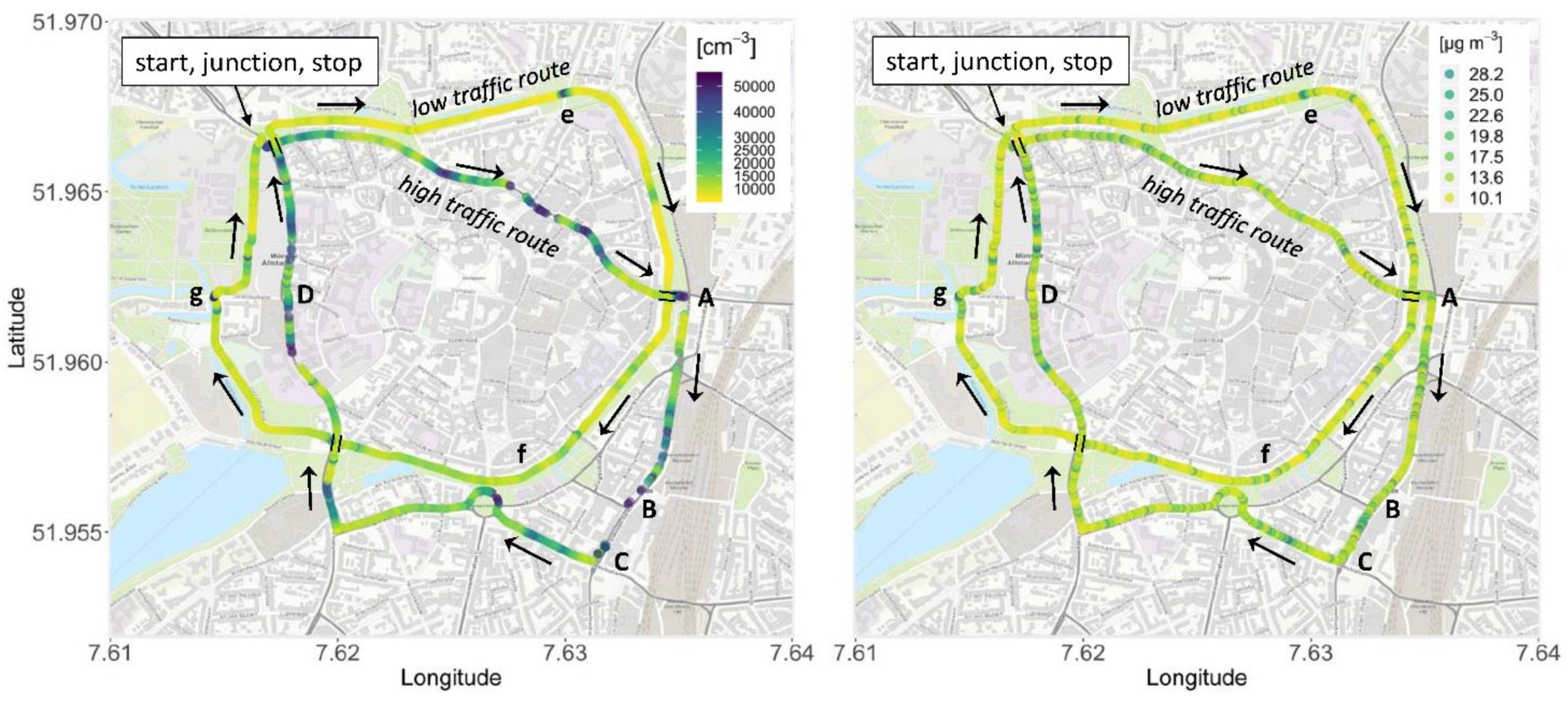
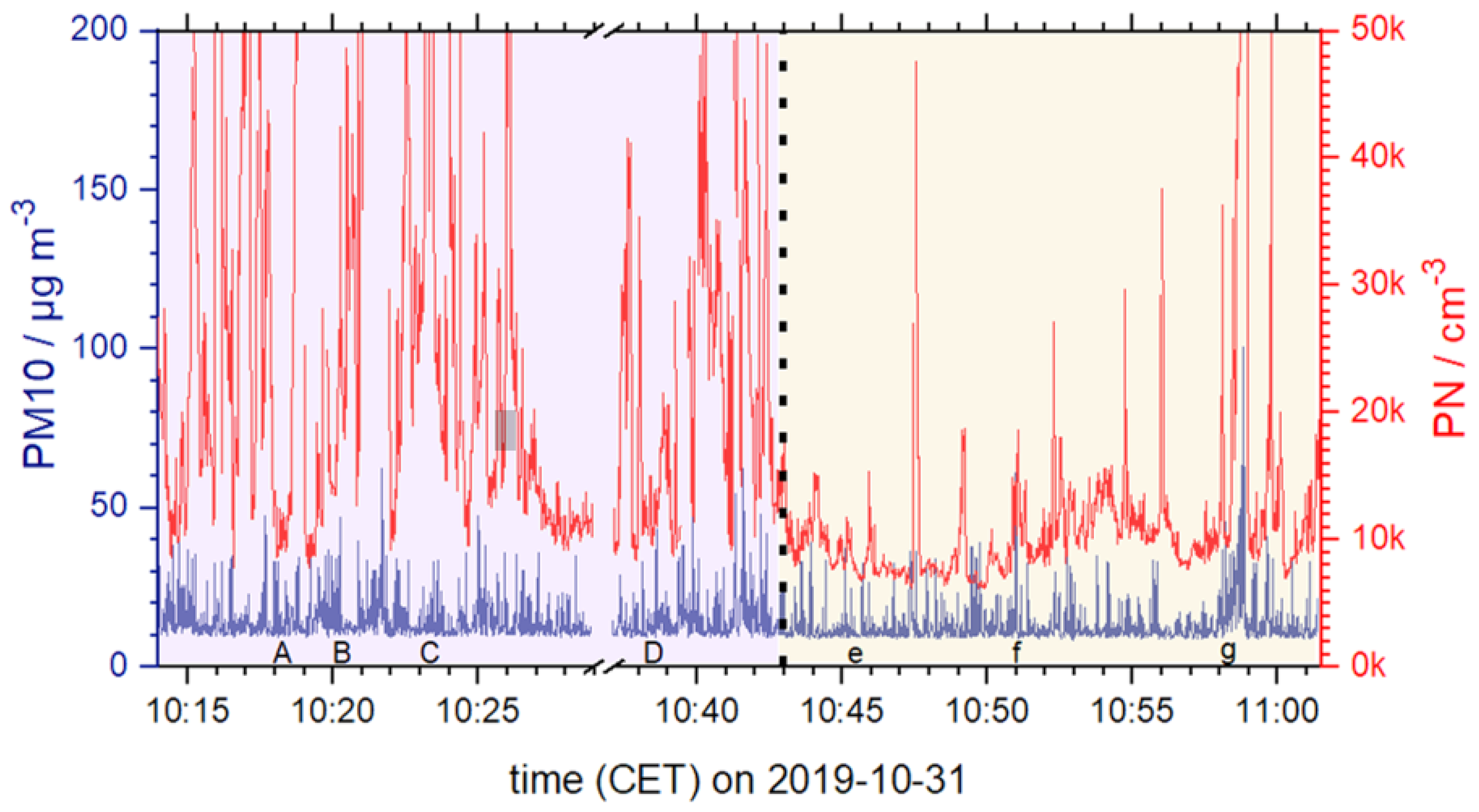
Table S2. As an example, the data for ride 3 on 31 October 2019 are shown in
Figure 3 and
Figure 4 for PN and PM10, respectively. The high-traffic route, which was the first lap of the ride, produced a large variability in PN concentrations. High spikes (>50,000 cm
−3) and phases of rather low concentrations (~10,000 cm
−3) occurred next to each other along the bike route. The maximum difference between neighboring data points—that is, from one second to the next and within about a 4 m horizontal distance—was 38,900 cm
−3. Clearly, the exhaust from motorized vehicles caused high variability whenever the instrumented bicycle came close to or within such plumes. Note that rather low concentrations also existed during this lap; the 10th percentile of PN concentrations was 10,400 cm
−3. The PN concentrations along the low-traffic route were generally much lower.
Here, the median (9600 cm
−3) was lower than the 10th percentile of the high-traffic route and concentrations above 15,000 cm
−3 were rare. However, episodes of high concentrations up to 17,700 cm
−3 also occurred when the low-traffic route passed arterial roads of the city, see point e in
Figure 3 (left panel) and
Figure 4 as an example. Overall, the differences in PN concentrations between the high-traffic route and the low-traffic route were large.
The PM10 concentrations between the high-traffic route and the low-traffic route during the same ride (
Figure 3, right panel,
Figure 4) also varied. The impact of road traffic on the PM10 concentrations is clearly recognizable for data points along the high-traffic route and from data points at intersections between the low-traffic route and arterial roads (e.g., point e in
Figure 3, right panel, and
Figure 4). The medians between the routes varied (11.4 vs. 9.9 µg m
−3) as did the interquartile ranges (9.87–14.9 µg m
−3 for the high-traffic route, 8.95–12.2 µg m
−3 for the low-traffic route), yet the differences between the routes were less pronounced than they were for the PN concentrations as discussed above, and they are non-significant. The spikes along the low-traffic route when intersecting arterial roads were recognizable yet quite small. The PM10 concentrations at the two urban air pollution monitoring sites during the time periods of bike rides were on average 23.6 µg m
−3 at MSGE and 23.9 µg m
−3 at VMS2, which is higher than the median concentrations of the cargo bicycle measurements, even larger than the respective third quartiles.
Figure 5 shows the ranges of the PN concentrations on the high-traffic route and the low-traffic route during all 40 rides. The differences between the PN concentration ranges were significant during all rides except rides 6 and 17. In most cases, the concentrations were higher on the high-traffic route than on the low-traffic route. Additionally, the overall PN concentrations were significantly higher on the high-traffic route as compared to the low-traffic route. Some exceptions were found for single rides: during ride 10 (on 10 April 2020), the PN concentrations were generally very high, often at or even above the upper detection limit of the CPC analyzer. This applied to both the high-traffic and the low-traffic route. Note that the latter showed even higher concentrations than the former.
For the PM10 and PM2.5 concentrations, some small differences were identified between the high-traffic routes and the low-traffic routes. For example, the PM10 medians were 10.0 and 9.2 µg m−3, respectively. For PM2.5, these medians were 4.7 and 4.3 µg m−3. The respective datasets are not significantly different from each other.
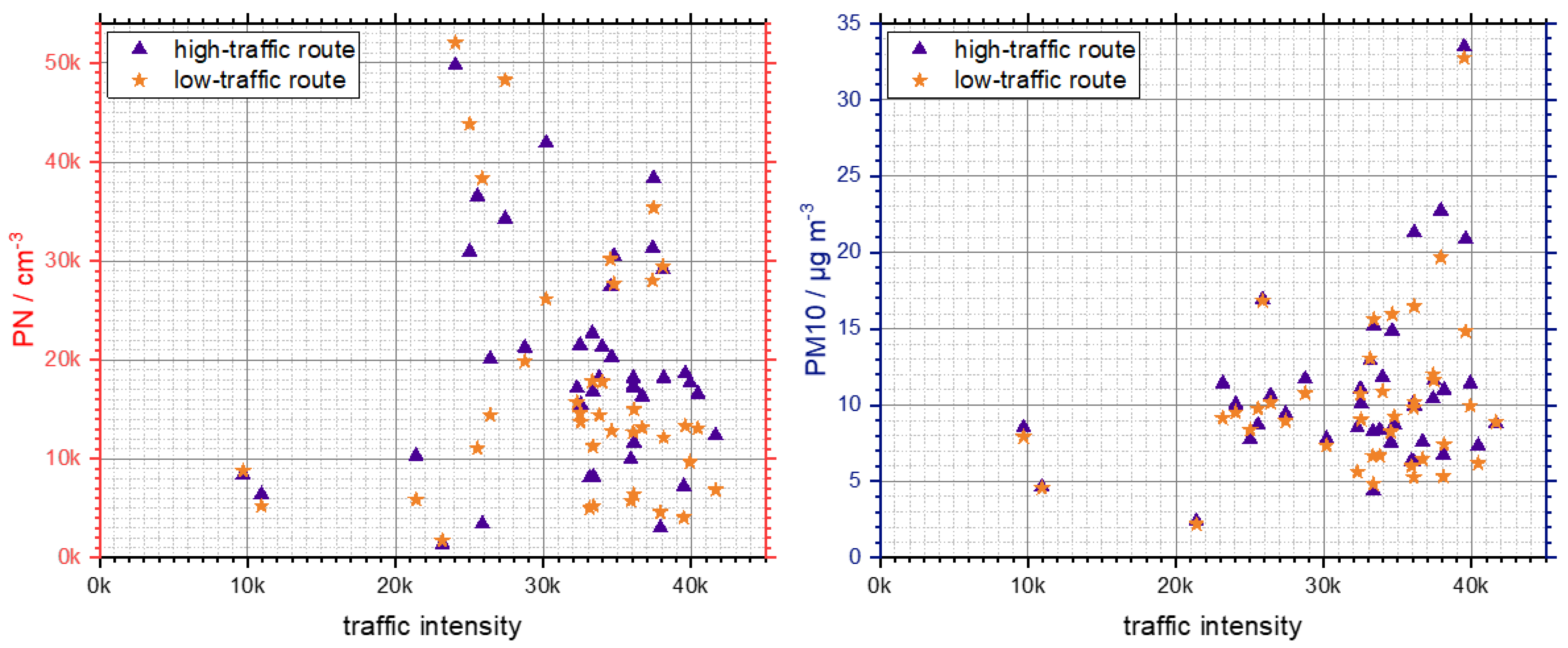
The medians of PN and PM10 during individual routes are shown aligned along the traffic intensity during the respective rides (x-axes) in
Figure 6. In both cases, no correlation between the parameters was found (likewise in the respective plots of PM2.5 and PM1, as well as in the 90th percentiles of all of these parameters, not shown). On the one hand, it seems convincing that low traffic intensities (below 24,500 for PN; below 22,500 for PM10) are strictly associated with low concentrations (<10,000 cm
−3 and <10 µg m
−3, respectively). On the other hand, such low concentrations also occurred all the way through the highest traffic intensities of over 40,000. Further, even medium traffic intensities (above the mentioned limits, up to ~35,000) yielded the highest (PN) or at least some of the higher (PM10) concentrations. For PM10, the highest concentrations occurred together with high traffic intensities, although these high traffic intensities also co-occurred with low PM10 (e.g., traffic intensity of 41,600 during ride 38 on 23 April 2021 together with 8.8 µg m
−3 on the high-traffic route and 8.9 µg m
−3 on the low-traffic route).
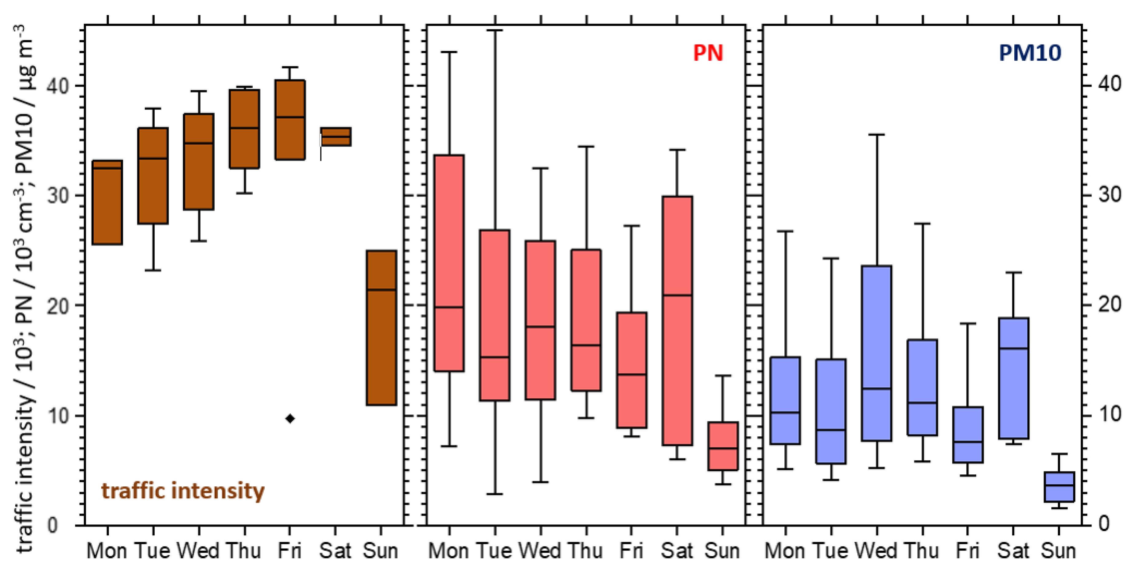
The weekly course of traffic intensity was very pronounced, with increasing traffic from Mondays through Fridays, while the weekends, especially Sundays, exhibited a drastic drop in traffic intensity (
Figure 7, left panel). Note that the statistical coverage of individual weekdays differs. There were only two rides on Saturdays and three rides on Sundays and Mondays each, while Tuesdays were represented by 10 rides. The PN and PM10 concentrations followed the weekly pattern in that the Sunday data were by far the lowest. Other than that, the interquartile ranges overlapped widely between all days (Mondays through Saturdays) and a systematic pattern was not apparent in the PN nor the PM10 data. The same applies for PM1 and PM2.5 (not shown).
The results of the relaimpo analysis (
Table 1) helped us integrate all findings into an overall picture. The explained variances of the medians and 90th percentiles of PN and PM10 were between 64% and 79%, which we consider a high percentage of explained variance within our real-world dataset. The PM1 and PM2.5 quantiles were predicted within the same range (not shown). The strongest predictor was the day of the week, explaining 26% of the variance of the 90th percentile of PM10 and 16% of its median. The very strong decrease in concentrations on Sundays (
Figure 6) impressively underlines this result.
The second single most important predictor was the choice of route for the 90th percentiles of PN (17%).
Figure 3 and
Figure 4 show large spikes of the PN concentrations along the high-traffic route, which apparently originated from a multitude of exhaust plumes from single motorized vehicles.
Some meteorological drivers also played important roles in the PN and PM concentrations. Specifically, the impact of the relative humidity (rH) on PN was strong (11.2% on the PN median; 9.2% on the 90th percentile). On average, PN concentrations decreased with increasing rH (details not shown). Another rather strong driver was the wind direction, affecting both the PN concentrations and the PM median. This was a surprising result considering the circular pattern of the travel routes. Moreover, the wind speed and the boundary layer stability had only minor impacts, which contradicts the general hypothesis of increasing air pollution levels with decreasing exchange conditions of the urban boundary layer.
Of the general air pollution data collected at the two state-operated sites VMS2 (a traffic site) and MSGE (an urban background site), the O3 concentration exerted the highest (statistical) impact on the particle concentrations measured with the instrumented bicycle. This indicates that superordinate, mesoscale processes may play important roles in establishing urban, street-level PN and PM concentrations.
Finally,
Table 1 also shows that the calendar day (day of the year) was not an important predictor of the measured PN and PM data. We address this rather non-intuitive result in the discussion section below.
4. Discussion
This contribution is a summary analysis of four student-led projects that analyzed the dynamics of aerosol particles in an urban setting. Initially, the study arose out of a course aiming to teach students about the impact of traffic and meteorology on air pollution by using a mobile platform. The course started in October/November 2019 as a practical class in urban meteorology at the undergraduate level with six participating students. After the course had ended, a nationwide lockdown led to a drastic reduction of public life in Germany. Under these circumstances, one of the participating students decided to add further measurements in April 2020 in order to broaden the variability of driving factors, specifically the traffic intensity, and aimed to describe the results in his bachelor’s thesis. The next-generation course (10 students, November 2020) decided to further expand the database because another, yet less efficient, lockdown, here called “lockdown light,” was enforced in late fall 2020. Although the subsequent full lockdown period during the Christmas and New Year holiday season of 2020/2021 was not covered by further data collection, another experimental period was added in April 2021 in order to complement the dataset with measurements from after-lockdown rides, thus allowing for a more extensive statistical analysis. This led to another bachelor’s thesis finalized in September 2021.
The 40 rides produced datasets including situations from very low to very high traffic intensities in the city (
Figure 2 and
Figure 6). In contrast to our initial assumptions, the general traffic intensity in town, which was derived from automatic traffic counts at traffic lights, was not of high importance for the PM10 nor the PN concentrations (
Table 1). Although very low traffic intensities yielded low PN and PM10 concentrations, such low particle concentrations also occurred at medium and high traffic intensities (
Figure 6). In summary, the choice of route (high traffic vs. low traffic) was important for the PN concentrations, especially for the occurrence of peaks with high concentrations, but it was of negligible importance for PM. Many diesel vehicles on the road still lack particle filters, thereby emitting large amounts of nano-sized particles [
10]; we presume these vehicles caused the observed pattern. These small particles contribute only a negligible fraction to the particle mass, specifically to the PM10 concentration, due to the cubic relationship between mass and number concentrations: With a spherical shape and identical densities, one particle with a 5 µm diameter has the same mass as a million particles each having a 50 nm diameter. This reasoning explains why the choice of the route has a much smaller impact on the PM10 concentrations (6.0% on the median, 3.1% on the 90th percentile). Data from ride 3, presented in
Figure 3 and
Figure 4, underline the large impact that the choice of route had on the PN concentrations, but the impact of route on the PM10 concentrations (as well as PM2.5 and PM1, not shown) was small.
Interestingly, the PM10 concentrations responded most to the day of the week (
Table 1), exhibiting by far the lowest concentrations on Sundays (
Figure 7). The traffic intensity was also low on Sundays. However, due to the reasoning provided above, it seems that the traffic intensity did not lead to the decreased PM10 on Sundays. We see two possible causes for the observed PM10 pattern, which may have acted alone or in combination: on the one hand, the PM10 concentration responds to non-exhaust traffic emissions, especially abrasion of brakes and tires [
10]. These emissions are closely related to heavy truck traffic, which is reduced to almost zero on Sundays. On the other hand, PM10 may respond to general commercial activity, specifically construction, which is also near zero on Sundays. The high percentiles of PM10 are associated with the background PM10 level in town (MSGE site,
Table 1), which provides some support for this argument.
The PN concentrations also responded to the weekday (low on Sundays,
Figure 7), yet we consider this to be a response to the absence of light-duty vehicles mainly from delivery companies, which emit very large numbers of nano-sized particles [
10].
A clear, general response of particle concentration (either PN or PM) to the traffic reduction during lockdown could not be proven (
Figure 6,
Table 1). Other studies showed for Germany and other sites in central Europe that the lockdown period in April/May 2020 exhibited a generally rather stable boundary layer with low wind speeds, which hindered very low air pollutant levels from being established [
43]. Although our results appear to be in good agreement with such more general findings, the fact that stability did not impact our PN concentrations and that the wind speed had relatively little influence on the 90th percentile of PM10 appears to be controversial.
The relative air humidity (rH) had a rather strong impact on the PN concentrations. High rH fosters the growth of nano-sized particles, which leads to faster coagulation and eventually to an efficient decrease in the particle number concentration [
45].
In addition to the general findings presented so far, here we also highlight some of the special observations we made. Ride 10 showed very high PN concentrations on both routes, the highest of all rides. The ride took place on Saturday, 10 April 2020, in which the traffic intensity was in a middle range of 24,000. This ride occurred within a very warm and sunny period after a rather cold spring season; except for a single day in February, the air temperature did not exceed 16 °C until four consecutive days just before 10 April, during which the daily maximum reached well above 18 °C, and it had reached over 22 °C on 6 and 8 April. These sudden warm spring conditions triggered many plant species to sprout. Although we did not observe the sprouting of Tilia cordata before 14 April 2020, we presume that the emission of volatile organic compounds (VOCs) from this and other species eventually led to intense secondary particle formation, which showed in the very high PN concentrations on both the high-traffic and the low-traffic routes.
We employed a 1 Hz time resolution of data acquisition during the bicycle rides. Some of the highest differences of concentrations happened for neighboring data points. For example, the PN concentrations jumped by over 40,000 cm−3 within 1 s (corresponding to about a 5 m distance) while cruising through the traffic circle in the south of the high-traffic route on 8 August 2020 at about 10:26 CET. In another case, the PM10 concentration jumped by over 600 µg m−3 within the same temporal and spatial frame when the bicycle passed a leaf blower on the low-traffic route on 14 April 2020, at 15:07 CET. Urban aerosol particle concentrations are extremely variable on short temporal and spatial scales, which should be considered in any future air pollution studies.
Finally, note that the day of the year only played a minor role in the relative importance analysis. We consider this finding to be counterintuitive because the seasons do play an important role in air pollution levels (see, for example,
Figure 2); particle concentrations in winter should be larger than those in summer. When re-inspecting the overall schedule of our four campaigns (
Figure 2), we found that neither the winter nor the summer seasons were covered. All our measurements were made either in late fall (2019 and 2020) or in spring (2020 and 2021), so only these transitional seasons were covered. Therefore, the absence of seasonal trends in our results is not a surprise.
5. Conclusions
The COVID-19 pandemic led to national lockdowns in Germany and other places in 2020 and 2021. As a result, the traffic intensity decreased significantly during these periods. We expected that these conditions as well as our specific experimental design (choice of routes of varying traffic intensity) would lead to clearly pronounced aerosol particle patterns. Yet, our hypotheses were only partly supported by the results. Motor traffic was not proven to be the main driver of particle concentrations (hypothesis i). The choice of route had some impact on aerosol concentrations (hypothesis ii), although its impact was stronger on the PN concentrations than on the PM concentrations (hypothesis iv). A general response to the urban traffic intensity could not be confirmed (hypothesis iii). The impact of boundary layer conditions and wind remains vague amid the incomplete coverage of seasons and the non-negligible response of PM10 to the wind speed.
While we found some rather clear responses to our hypotheses, we also found that the dynamics of aerosol particles in the urban space were established and driven within a multidimensional space, which cannot be analyzed with simple or even multiple linear regressions in a satisfactory fashion. We suggest improvements and extensions of both the measurement strategies and the data analysis tools to further improve our understanding. First, in order to improve the understanding of the role of motorized street traffic, the concentrations of nitrogen oxides need to be incorporated in future similar experiments; suitable analytical instruments for use on cargo bicycles are available today [
46]. Second, the data analysis needs to focus more on further available data such as the CO
2 concentrations. Third, a much larger dataset needs to be created that better covers the seasons of the year, the human activity (weekdays, holidays, etc.), time of day, etc. Fourth, researchers should consider excluding data from arterial road intersections on the low-traffic-route in order to exclude from this dataset the influence of motorized street traffic. Finally, we believe that an identification of individual motorized vehicles near the bicycle through video observation and license plate identification would be very useful in order to quantify the share of gasoline, diesel, and electric vehicles and the types of vehicles (e.g., car, bus, low-duty vehicle). This information would be very helpful in understanding the measured peak concentrations [
10]. It is, however, difficult to obtain appropriate permits for video surveillance in public spaces under current general data protection regulations in the European Union.
Last, but not least, we believe that the dynamics of aerosol particles in urban areas of Germany will undergo rapid changes within the next few years as the share of electro-mobility increases in response to air pollution control and climate adaptation efforts. Nevertheless, air pollution is, as mentioned above, still “the biggest environmental health risk” in Europe [
2], and we need well-educated and well-trained university graduates to meet these challenges in the medium and long term.


 ,
, 


