
Global Dynamics of a Discrete-Time MERS-Cov Model


1
Department of Basic Sciences, Princess Sumaya University for Technology, Amman 11941, Jordan
2
Department of Mathematics, The Hashemite University, Zarqa 13133, Jordan
3
Department of Mathematics, University of Jordan, Amman 11942, Jordan
*
Author to whom correspondence should be addressed.
†
These authors contributed equally to this work.
Mathematics 2021, 9(5), 563; https://doi.org/10.3390/math9050563
Submission received: 26 January 2021
/
Revised: 28 February 2021
/
Accepted: 4 March 2021
/
Published: 6 March 2021
Abstract
:In this paper, we have investigated the global dynamics of a discrete-time middle east respiratory syndrome (MERS-Cov) model. The proposed discrete model was analyzed and the threshold conditions for the global attractivity of the disease-free equilibrium (DFE) and the endemic equilibrium are established. We proved that the DFE is globally asymptotically stable when . Whenever , the proposed model has a unique endemic equilibrium that is globally asymptotically stable. The theoretical results are illustrated by a numerical simulation.
1. Introduction
Mankind has been suffering from several epidemic diseases during every age of human being history. In the past century, many disease outbreaks have occurred, such as influenza, malaria, dengue fever, SARS, H1N1, H7N1, pestilence, AIDS, MERS and Covid-19. Recently, most of the viruses that affect the mankind life are the coronaviruses, which are a single standard RNA virus that were firstly reported in 1960s [1].
Severe acute respiratory syndrome (SARS) is an airborne virus which was firstly found in Foshan, China on 16 November 2002 [2]. The spread of the SARS virus was through small droplets of saliva, similar to influenza with an incubation period of 2–7 days. The SARS virus transmission was from bats to humans. The number of reported cases was 8098 and the number of death cases was 774 [3]. The middle east respiratory syndrome (MERS) is a viral respiratory disease caused by novel coronavirus MERS-Cov, that was first reported in Saudi Arabia in 2012 [4]. The infection of MERS may occur through both animals, such as camels and bats, and humans by a direct or indirect contact [5]. The incubation period of MERS is 2 to 14 days [6]. Since 2012, the reported infected cases of MERS are 2494 with a death rate of 34% [7]. In early December 2019, the first case of Covid-19 was reported in Wuhan, China [8]. The symptoms of Covid-19 are similar to the other coronaviruses SARS and MERS, such as colds and high temperature, which lead to pneumonia and hence respiratory system failure and death [9].
A vast number of mathematical models have been proposed to understand the dynamics of the coronaviruses. The SIS, SIR and SEIR models are studied by many researchers to investigate the dynamics of the coronaviruses [10,11,12,13,14,15,16,17,18,19,20,21,21]. The model we have proposed in this paper is investigating the dynamics of the middle east respiratory syndrome coronavirus. We have studied the asymptomatic, symptomatic and hospitalized individuals’ effects on the spread of the virus.
Yong and Owen [22] have discussed the dynamical transmission model of MERS-Cov in two areas. They proved that the model has two equilibrium points, a disease-free equilibrium point and an endemic equilibrium point. Moreover, the disease dies out whenever the basic reproductive number is less than unity. Usaini et al. [17] proposed a new deterministic mathematical model for the transmission dynamics of MERS-Cov. They found that there is a unique endemic equilibrium point and there is no infection free equilibrium point due to the constant influx of latent immigrants. Lee et al. [16] have designed a dynamic transmission model to analyze the MERS-Cov outbreak in the Republic of Korea. This model incorporates the time-dependent parameters and the pulse of infections. Moreover, they estimated the basic reproductive number, , and showed that it is decreased which indicates that the MERS-Cov outbreak in the Republic of Korea had a low transmissibility.
Scientists have studied several types of dynamical epidemic models such as continuous-time type models that are described by differential equations and discrete-time type models that are described by difference equations. Currently, the scientists have paid more attention to the investigation of bigdata, which have made the discrete-time type epidemic models more interesting. In addition, discrete-time models have more dynamical behaviors [23].
Numerous studies have been done to explore the discrete-time epidemic models. L. Wang et al. [23] have studied a class of discrete SIRS epidemic models with disease courses. The authors have computed the basic reproduction number . In addition, they have proved that the disease-free equilibrium is globally attractive when and the disease is permanent whenever . Y. Wang et al. [24] have introduced Lyapunov functions for a class of discrete SIRS epidemic models with nonlinear incidence rate and varying population size. The authors have established the sufficient and necessary conditions on the global asymptotic stability of the disease-free equilibrium and endemic equilibrium with general nonlinear incidence rate and different death rates. X. Fan et al. [25] have investigated a class of SEIRS epidemic models with a general nonlinear incidence function. In addition, they considered a discrete SEIRS model with standard incidence function. Moreover, the authors have shown that the model has a disease-free equilibrium, is globally attractive when the basic reproduction number and the disease is permanent whenever . Batarfi et al. [18] have proposed a nonlinear mathematical model for MERS-Cov with two discrete-time delays. They computed the reproduction number, , and proved that there exists a disease-free equilibrium point when and there is an endemic equilibrium point whenever . M. Khan et al. [26] have investigated a discrete-time TB model which is parameterized by the cases in the Pakistani of Khyber Pakhtunkhwa between 2002 and 2017. The authors have computed the reproduction number which showed that the discrete-time TB model is stable at the disease-free equilibrium point when and the model is globally asymptotically stable for the endemic equilibrium point whenever . Moreover, the authors have compared the discrete-time model with the continuous-time model. M. Safi et al. [27] have considered a discrete-time mathematical model that is obtained from the continuous-time model in [28]. The authors investigated the stability of the model and they proved that the model is globally asymptotically stable when .
This paper is organized as follows: A discrete MERS-Cov epidemic model is considered in Section 2. In Section 3, we present the fundamental properties of the discrete model. The stability analysis of the disease-free equilibrium is carried out in Section 4. The existence and stability analysis of endemic equilibrium point is conducted in Section 5. In Section 6, numerical simulations are provided to illustrate the obtained results and the results are concluded.
2. Model Formulation
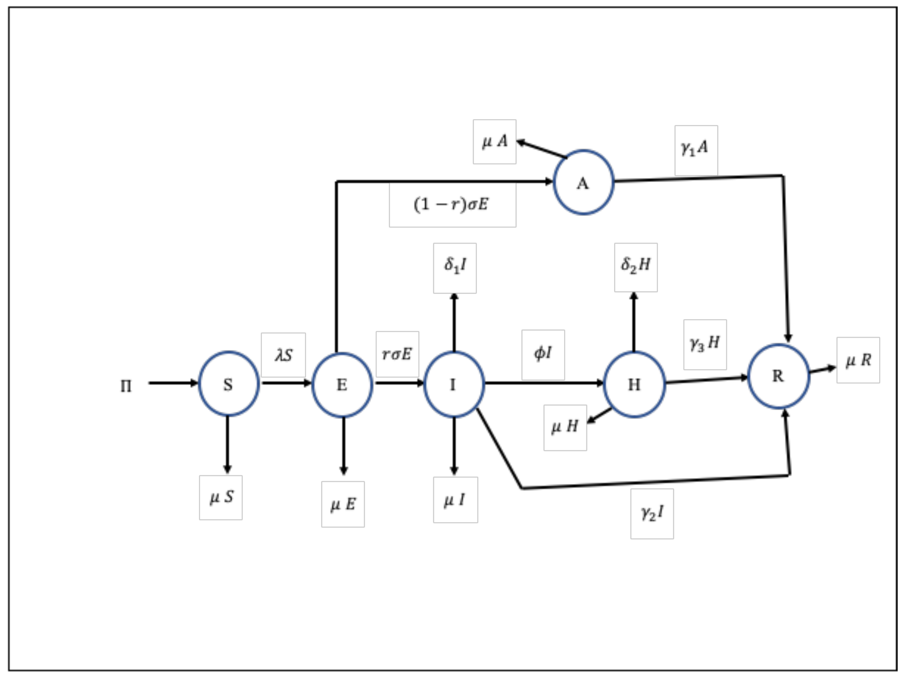
The backward difference scheme is applied to propose the following discrete epidemic MERS-Cov coronavirus model. This model is called SEAIHR model. The population is divided into the following compartments: is the susceptible individuals, is the exposed individuals, is the asymptomatic individuals, is the symptomatic individuals, is the hospitalized individuals and is the recovered individuals. Hence, . Susceptible people (S) is increased by the recruitment of individuals into the population, at a rate of . This class is decreased by infection (with the rate of ). Furthermore, this population is decreased by natural death (at a rate of ; populations in all classes are assumed to have the same natural death rate). Exposed individuals (E) are generated with the rate of and reduced by progression to the asymptomatic individuals (A) at rate of and to the symptomatic individuals (I) at rate of (r). The class of asymptomatic individuals (A) increased to the exposed individuals at a rate of and it is reduced by progression to the exposed at rate of (r) and to the recovered individuals (R) at rate of . The symptomatic class (I) is increased by the exposed people at a rate of () and decreased to the hospitalized individuals (isolation) (H) at rate of , to the recovered people at rate of and disease-induced death (at a rate ). The hospitalized (isolated) class is increased by the symptomatic individuals (I) at rate of and decreased to recovery at rate of and disease-induced death (at a rate ). Figure 1 illustrates the model (1) by a schematic diagram. Therefore, the SEAIHR model is governed by the following difference equations:
where , , , , , is the recruitment rate of susceptible people corresponding to births and immigration, is the natural death rate, is the contact rate, is the mean time of incubation period, is the mean time from data of symptoms onset to data of hospitalization, r is the clinical outbreak rate in all the infected cases, is the mean infections period of asymptomatic infected person for survivors, is the mean duration of infected person for survivors, is the mean duration for hospitalized cases for survivors and is the disease-induced death rate of infectious. Subject to the following initial conditions:
It is worthy to mention that such models are potentially analytically solvable by using the Lie algebra method through matrix exponentials [29]. Based on the Kolmogorov equation and the Wei–Norman method, the analytical solution for the proposed model can be obtained in terms of matrix exponentials (for more details about Lie algebra method, see [30,31]).
3. Fundamental Properties
To prove Lemma 1, we will apply the mathematical induction as follows:
Proof.
Let . Hence, we define
Let , , , , and . Then, Equation (5) can be written as follows:
Which is simplified to
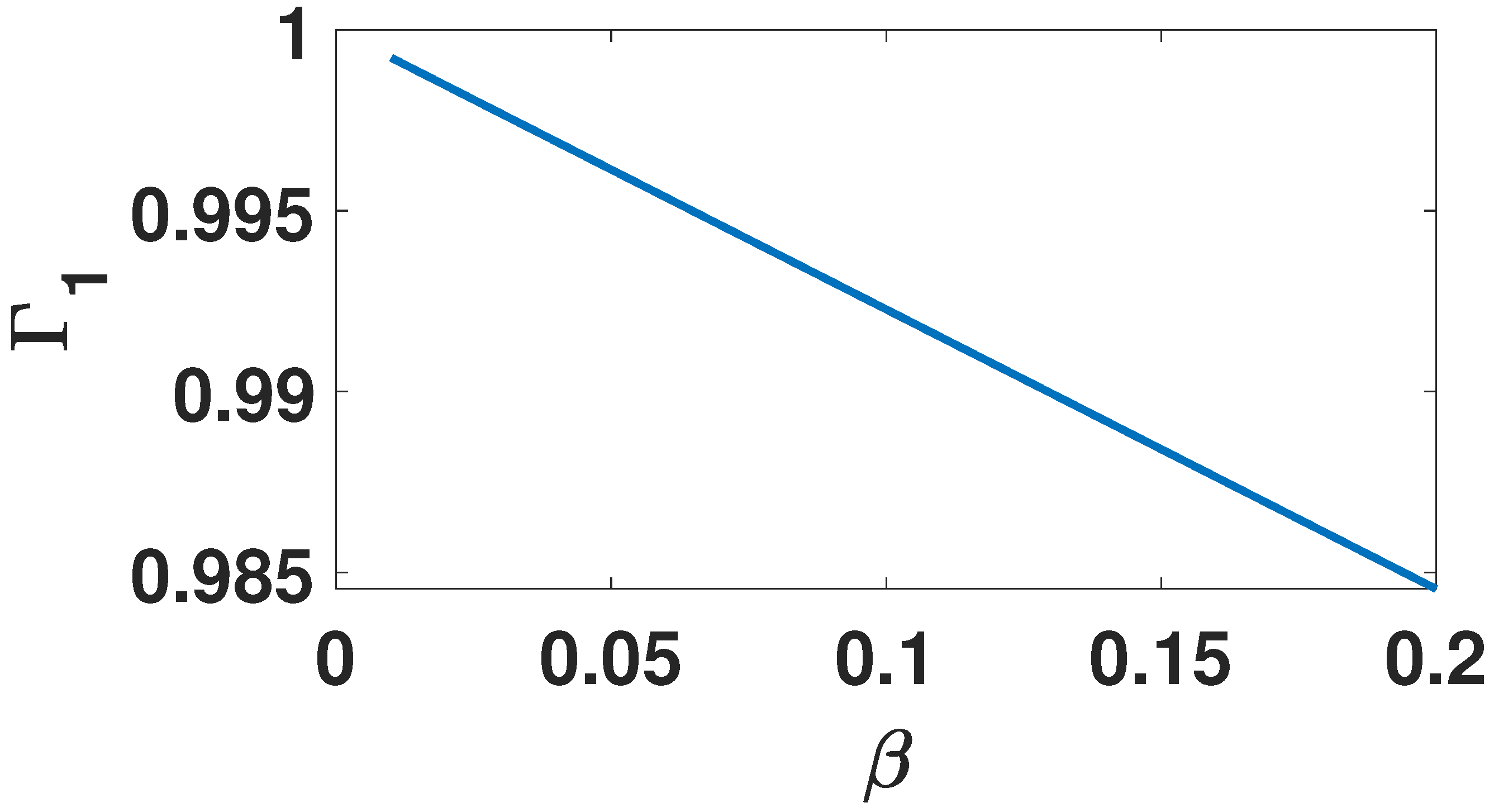
where , and . Since , see Figure 2, then . Moreover, and hence, , then is an increasing function and , then has a unique positive solution and therefore, Equation (4) has a unique solution which implies that a unique , , and exist with , , and .
Let . Thus, from the first equation in model (1), we define
where . Since is continuous and , then is an increasing function with . Thus, by the intermediate value theorem has a unique positive solution and therefore, there exists a unique which completes the proof. □
Proof.
Since,
Hence,
□
Therefore, the region
is positively invariant.
4. Disease-Free Equilibrium (DFE)
4.1. Local Stability of DFE
The unique disease-free equilibrium (DFE) of the system (1) is given by
To compute the basic reproduction number of model (1), we will apply the next generation operator method [32,33,34,35,36]. The matrix of the new infection terms, F, and the matrix of the transition terms, V, that are associated with the model (1) are given by:
Following [34], the basic reproduction number is denoted by and is given by
The proof of following lemma can be deduced from the proof of Theorem 2 in [34], which is the following “Consider the disease transmission model given by (1). If is a disease-free equilibrium of the model, then is locally asymptotically stable if , but unstable if , where .”
Lemma 3.
The DFE point of model (1) is locally asymptotically stable (LAS) when and unstable when .
4.2. Global Stability of DFE
In this section, the global attractivity of the disease-free equilibrium of model (1) is investigated and we can obtain the following result.
Theorem 1.
The DFE of the model (1) is globally-asymptotically stable (GAS) in whenever
Proof.
Consider the following Lyapunov function
where
The backward difference of is denoted by and is given by
This implies that and if and only if . Hence, as . Upon setting in the first and last equations in model (1), we get and as . Thus, the maximum invariable set in is a disease-free equilibrium . Following the theorems of stability of difference equations (Theorem 6.3 in [36]), every solution of the equations in model (1) with the initial conditions in approaches as . Thus, the disease-free equilibrium of model (1) is globally attractive. Hence, the proof is completed. □
It is worthy to remark that similar techniques have been used in the proof of stability with feedback (for more details see [37]).
5. Endemic Equilibria
5.1. Existence of the Endemic Equilibrium Point EEP
Let be and endemic equilibrium point for the model (1). Hence, we can conclude the following lemma.
Lemma 4.
The model (1) has a unique endemic equilibrium point , whenever .
5.2. Stability of the Endemic Equilibrium
Although no global asymptotic stability result is given here for the endemic equilibrium point , extensive numerical simulations suggest that is a GAS in , whenever . Hence, we add the following conjecture.
Conjecture 1.
The unique endemic equilibrium point (EEP) of the model (1) is globally asymptotically stable (GAS) in if .
For mathematical convenience, we provide the proof of the conjecture (1) for the special case when the associated disease-induced mortality is neglected, i.e, . Therefore, we define
which is the basin of attraction of the disease-free equilibrium point , to conduct the global stability of the unique endemic equilibrium point for this case. Hence, the following result is obtained.
Theorem 2.
The unique endemic equilibrium point (EEP) of the model (1) with is globally asymptotically stable (GAS) in if
6. Discussion and Conclusions
In this section, we will investigate the numerical simulation of the proposed model (1). The values of the model (1) parameters are listed in Table 1 below.
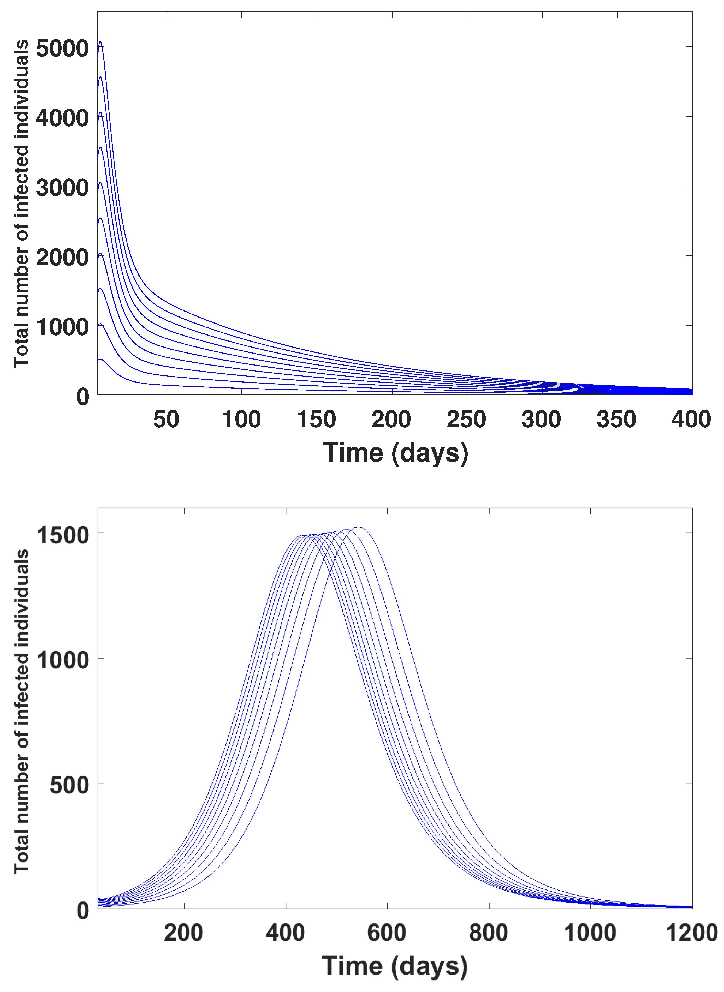
Figure 3 (Up) shows that the disease dies out which means that the disease-free equilibrium point of model (1) is globally attractive and Figure 3 (Down) shows that the disease is permanent.
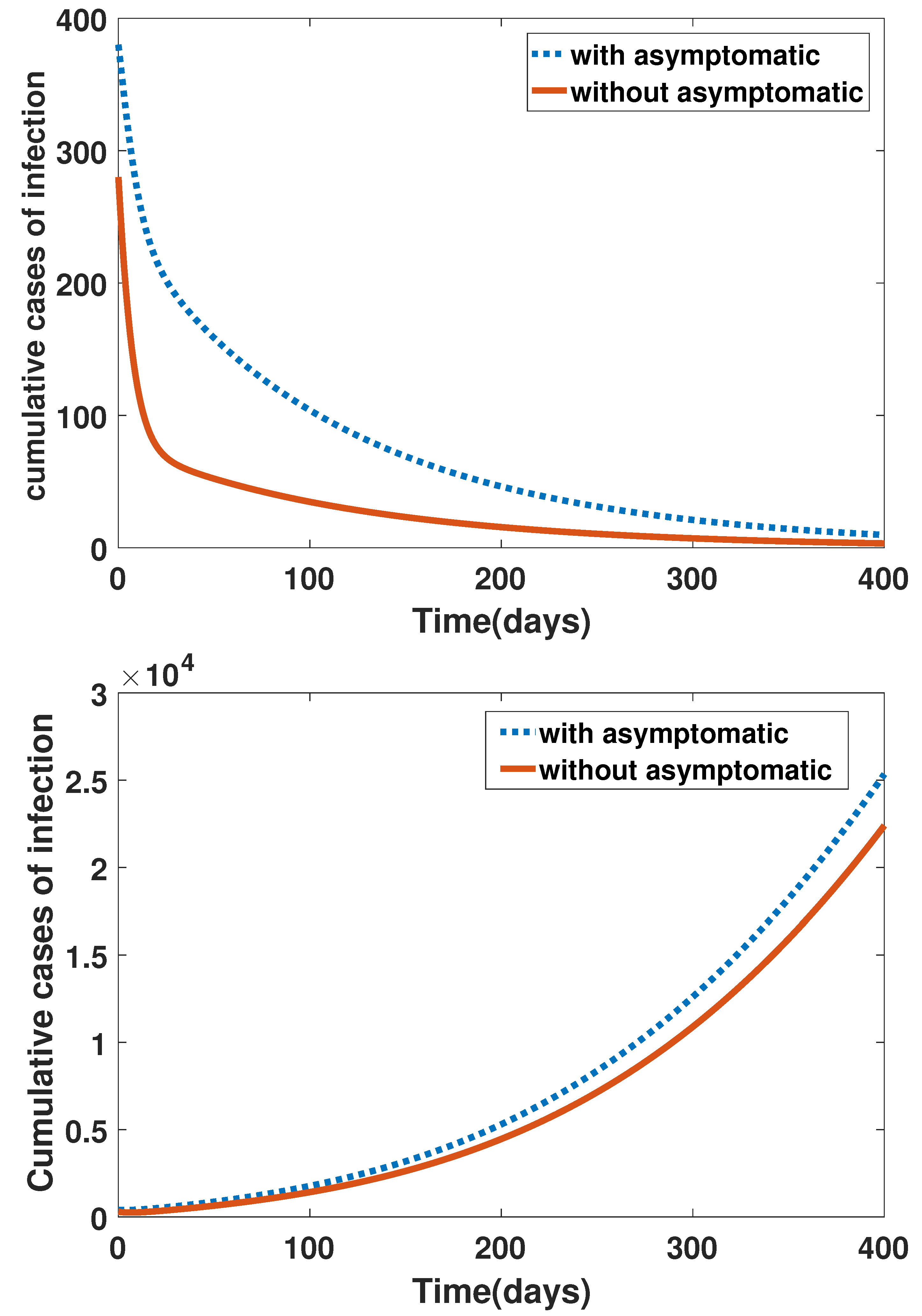
Figure 4 displays that the number of cumulative cases of infection with treatment is larger than cumulative cases of infection without treatment.
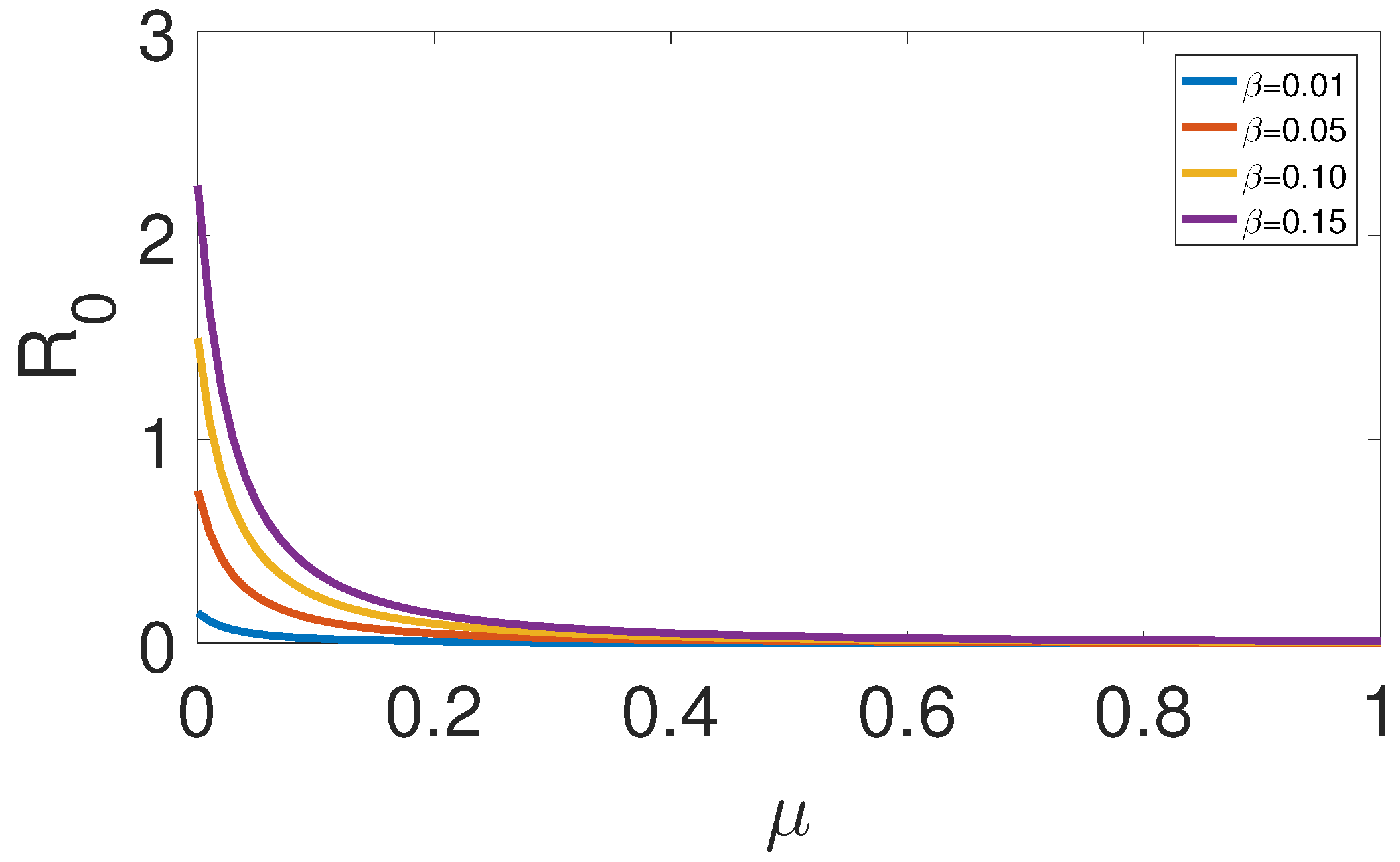
Figure 5 depicts the relation between the basic reproduction number and the natural death rate for several values of the contact rate . It shows that decreases as increases and increases as increases.
Author Contributions
Conceptualization, M.H.D. and M.A.S.; methodology, M.H.D. and M.A.S.; software, M.A. and M.H.D.; validation, M.H.D., M.A.S. and M.A.; formal analysis, M.H.D. and M.A.S.; writing—original draft preparation, M.H.D.; writing—review and editing, M.H.D.; visualization, M.H.D.; supervision, M.H.D.; project administration, M.H.D. All authors have read and agreed to the published version of the manuscript.
Funding
This research received no external funding.
Institutional Review Board Statement
Not applicable.
Informed Consent Statement
Not applicable.
Data Availability Statement
The data used to support the findings of this study are included in the references within the article.
Acknowledgments
The authors are grateful to the anonymous reviewers for their constructive comments.
Conflicts of Interest
The authors declare no conflict of interest.
Abbreviations
The following abbreviations are description of variables and parameters of the model (1).
| Variable | Description |
| Population of susceptible individuals | |
| Population of exposed individuals | |
| Population of asymptotic individuals | |
| Population of symptotic individuals | |
| Population of hospitalized individuals | |
| Population of recovered individuals | |
| Parameter | Description |
| Recruitment rate | |
| Natural death rate | |
| r | The clinical outbreak rate |
| Contact rate | |
| The mean time of incubation period | |
| The mean time from symptoms to hospitalization | |
| The reduction factor in transmission rate by symptomated per day | |
| The reduction factor in transmission rate by hospitalized per day | |
| The mean infections period of asymptomatic infected person for survivors | |
| The mean duration of infected person for survivors | |
| The mean duration for hospitalized cases for survivors | |
| Disease-induced death rate of infectious individuals | |
| Disease-induced death rate of treated individuals |
References
- Khan, J.S.; Mclntosh, K. History and recent advances in coronavirus discovery. Pediatr. Infect. Dis. J. 2005, 24, 16378050. [Google Scholar] [CrossRef] [PubMed]
- A chronicle on the SARS epidemic. Chin. Law Gov. 2003, 36, 12–15. [CrossRef]
- Chan-Yeung, M.; Xu, R. SARS epidemiology. Respirology 2003, 8, 9–14. [Google Scholar] [CrossRef] [PubMed]
- Al-Tawfiq, J.; Smallwood, C.; Arbuthnott, K.; Malik, M.S.; Barbeschi, M.; Memish, Z. Emerging respiratory and novel coronavirus 2012 infections and mass gatherings. East. Mediterr. Health J. 2012, 19, 48–54. [Google Scholar] [CrossRef]
- World Health Organization. Middle East Respiratory Syndrome Coronavirus (MERS-Cov); World Health Organization: Geneva, Switzerland, 2019. [Google Scholar]
- Mackay, T.M.; Arden, K.E. MERS coronavirius: Diagnostics epidemology and transmissions. Proc. R Soc. Lond. B 2015, 12, 222. [Google Scholar]
- The Kingdome of Saudi Arabia. Middle East Respiratory Syndrome Coronavirus (MERS-Cov); The Kingdome of Saudi Arabia: Riyadh, Saudi Arabia, 2019. [Google Scholar]
- World Health Organization. World Health Organization Coronavirus; World Health Organization: Geneva, Switzerland, 2020. [Google Scholar]
- Zhu, Z.; Lian, X.; Su, X.; Wu, W.; Marearo, G.; Zeng, Y. From SARS and MERS to Covid-19: A brief summary and comparison of severe acute respiratory infections caused by three highly pathogenic human coronaviruses. Respir. Res. 2020, 21, 224. [Google Scholar] [CrossRef]
- He, S.; Peng, Y.; Sun, K. SEIR modeling of the covid-19 and its dynamics. Nonlinear Dyn. 2020, 101, 1667–1680. [Google Scholar] [CrossRef]
- Ellison, G. Implications of the Heterogeneous SIR Models for Analyses of Covid-19; NBER Working Papers 27373; National Bureau of Economic Research, Inc.: Cambridge, MA, USA, 2020. [Google Scholar]
- Law, K.B.; Peariasamy, K.M.; Gill, B.S. Tracking the early depleting transmission dynamics of Covid-19 with a time-varying SIR model. Sci. Rep. 2020, 10, 21721. [Google Scholar]
- Ng, T.W.; Turinic, G.; Danchin, A. A double epidemic model for the SARS propagation. BMC Infect. Dis. 2003, 3, 19. [Google Scholar] [CrossRef] [PubMed]
- Yu, J.; Jiang, D.; Shi, N. Global stability of two-group SIR model with random perturbation. J. Math. Anal. Appl. 2009, 360, 235–244. [Google Scholar] [CrossRef] [Green Version]
- Hu, Z.; Ma, W.; Ruan, S. Analysis of SIR epidemic models with nonlinear incidence rate and treatment. Math. Biosci. 2012, 238, 12–20. [Google Scholar] [CrossRef]
- Lee, J.; Chowell, G.; Jung, J. A dynamic compartmental model for the Middle East respiratory syndrome outbreak in the Republic of Korea: A retrospective analysis on control interventions and superspreading events. J. Theor. Biol. 2018, 408, 118–126. [Google Scholar] [CrossRef] [Green Version]
- Usaini, S.; Hassan, A.S.; Garba, S.M.; Lubuma, J.M.-S. Modeling the transmission dynamics of the Middle East Respiratory Syndrome Coronavirus (MERS-CoV) with latent immigrants. J. Interdiscip. Math. 2019, 22, 903–930. [Google Scholar] [CrossRef] [Green Version]
- Batarfi, H.; Elaiw, A.; Alshareef, A. Dynamical behavior of MERS-COV model with discrete delays. J. Comput. Anal. Appl. 2019, 26, 37–49. [Google Scholar]
- Alshareef, A.; Elaiw, A. Dynamical behavior of MERS-COV model with distributed delays. Appl. Math. Sci. 2019, 13, 283–298. [Google Scholar] [CrossRef] [Green Version]
- Chowell, G.; Blumberg, S.; Simonsen, L.; Miller, M.; Viboud, C. Synthesizing data and models for the spread of MERS-COV, 2013: Key role of index cases and hospital transmission. Epidemics 2014, 9, 40–57. [Google Scholar] [CrossRef] [PubMed] [Green Version]
- DarAssi, M.H.; Safi, M.A.; Al-Hdaibat, B. A delayed SEIR epidemic model with pulse vaccination and treatment. Nonlinear Stud. 2018, 25, 1–16. [Google Scholar]
- Yong, B.; Owen, L. Dynamical transmission model of MERS-Cov in two areas. AIP Conf. Proc. 2016, 1716, 020010. [Google Scholar] [PubMed]
- Wang, L.; Cui, Q.; Teng, Z. Global dynamics in a class of discrete-time epidemic models with disease courses. Adv. Differ. Equ. 2013, 2013, 57. [Google Scholar] [CrossRef] [Green Version]
- Wang, Y.; Teng, Z.; Rehim, M. Lyapunov functions for a class of discrete SIRS models with nonlinear incidence rate and varying population sizes. Discret. Dyn. Nat. Soc. 2014, 2014, 1–10. [Google Scholar] [CrossRef]
- Fan, X.; Wang, L.; Teng, Z. Global dynamics for a class of discrete SEIRS epidemic models with general nonlinear incidence. Adv. Differ. Equ. 2016, 2016, 123. [Google Scholar] [CrossRef] [Green Version]
- Khan, M.A.; Khan, K.; Safi, M.A.; DarAssi, M.H. A Discrete Model of TB Dynamics in Khyber Pakhtunkhwa-Pakistan. Comput. Model. Eng. Sci. 2020, 123, 777–795. [Google Scholar]
- Safi, M.A.; Al-Hdaibat, B.; DarAssi, M.H.; Khan, M.A. Global dynamics for a discrete quarantine/isolation model. Rersults Phys. 2021, 21, 103788. [Google Scholar]
- Safi, M.A.; Gumel, A.B. Global asymptotic dynamics of a model for quarantine and isolation. Discret. Contin. Dyn. Syst. B 2010, 14, 209–231. [Google Scholar]
- Shang, Y. Lie algebra method for solving biological population model. J. Theor. Appl. Phys. 2013, 7, 67. [Google Scholar] [CrossRef] [Green Version]
- Shang, Y. Analytical solution for an in-host viral infection model with time-inhomogeneous rates. Acta Phys. Pol. B 2015, 46, 1567–1577. [Google Scholar] [CrossRef] [Green Version]
- Shang, Y. Lie algebraic discussion for affinity based information diffusion in social networks. Open Phys. 2017, 15, 705–711. [Google Scholar] [CrossRef]
- Anderson, R.M.; May, R.M. Population Biology of Infectious Diseases; Springer-Verlag: Berlin/Heidelrberg, Germany; New York, NY, USA, 1982. [Google Scholar]
- Diekmann, O.; Heesterbeek, J.A.P.; Metz, J.A.J. On the definition and computation of the basic reproduction ratio R0 in models for infectious disease in heterogeneous population. J. Math. Biol. 1990, 28, 365–382. [Google Scholar]
- van den Driessche, P.; Watmough, J. Reproduction numbers and subthreshold endemic equilibria for compartmental models of disease transmission. Math. Biosci. 2002, 180, 29–48. [Google Scholar] [CrossRef]
- Hethcote, H.W. The mathematics of infectious diseases. SIAM Rev. 2000, 42, 599–653. [Google Scholar] [CrossRef] [Green Version]
- LaSalle, J.P. The Stability of Dynamical Systems; SIAM: Philadelphia, PA, USA, 1976. [Google Scholar]
- Shang, Y. Global stability of disease-free equilibria in a two-group SI model with feedback control. Nonlinear Anal. Model. Control. 2015, 20, 501–508. [Google Scholar] [CrossRef] [Green Version]
Figure 1.
Model (1) schematic diagram.
Figure 1.
Model (1) schematic diagram.

Figure 2.
The plot of the the cofactor as a function of .

Figure 3.
The infected compartments as functions of time when (Up). The infected compartments as functions of time when (Down).
Figure 3.
The infected compartments as functions of time when (Up). The infected compartments as functions of time when (Down).

Figure 4.
The plot of the cumulative cases of infection verses time in days with treatment (dotted line) and without treatment (solid line) when (Up). The plot of the cumulative cases of infection verses time in days with treatment (dotted line) and without treatment (solid line) when (Down).
Figure 4.
The plot of the cumulative cases of infection verses time in days with treatment (dotted line) and without treatment (solid line) when (Up). The plot of the cumulative cases of infection verses time in days with treatment (dotted line) and without treatment (solid line) when (Down).

Figure 5.
The plot of the basic reproduction number as a function of the birth–death rate for several values of the contact rate.
Figure 5.
The plot of the basic reproduction number as a function of the birth–death rate for several values of the contact rate.


Table 1.
The values of the parameters of model (1) when and when .
Table 1.
The values of the parameters of model (1) when and when .
| Parameter | Parameter | ||||
|---|---|---|---|---|---|
| 136 | 136 | 0.0337 | 0.0337 | ||
| 0.000035 | 0.000035 | 0.0486 | 0.0486 | ||
| r | 0.5 | 0.5 | 0.0535 | 0.0535 | |
| 0.05 | 0.10 | 0.1 | 0.1 | ||
| 0.157 | 0.157 | 0.1 | 0.1 | ||
| 0.2 | 0.2 | 0.03 | 0.03 | ||
| 0.04 | 0.04 |
Publisher’s Note: MDPI stays neutral with regard to jurisdictional claims in published maps and institutional affiliations. |
© 2021 by the authors. Licensee MDPI, Basel, Switzerland. This article is an open access article distributed under the terms and conditions of the Creative Commons Attribution (CC BY) license (http://creativecommons.org/licenses/by/4.0/).
Share and Cite
MDPI and ACS Style
DarAssi, M.H.; Safi, M.A.; Ahmad, M. Global Dynamics of a Discrete-Time MERS-Cov Model. Mathematics 2021, 9, 563. https://doi.org/10.3390/math9050563
AMA Style
DarAssi MH, Safi MA, Ahmad M. Global Dynamics of a Discrete-Time MERS-Cov Model. Mathematics. 2021; 9(5):563. https://doi.org/10.3390/math9050563
Chicago/Turabian StyleDarAssi, Mahmoud H., Mohammad A. Safi, and Morad Ahmad. 2021. "Global Dynamics of a Discrete-Time MERS-Cov Model" Mathematics 9, no. 5: 563. https://doi.org/10.3390/math9050563
Note that from the first issue of 2016, this journal uses article numbers instead of page numbers. See further details here.