


Introduction
In December 2019, a disease that appeared in central China precisely in the city of Wuhan (Hubei Province) started to take its toll. On 7 January 2020, Chinese authorities admitted that the country was facing an epidemic caused by a new virus from the coronavirus family. First named ‘2019-nCOV’, this virus and disease was named COVID-19 or SARS-CoV-2 by the World Health Organization (WHO) [1]. COVID-19 disease has passed in a few weeks from a localised epidemic to a pandemic. This disease is now a public health emergency at the international level and is currently affecting more than 200 countries with more than 350 000 deaths and nearly 6 million people infected according to the WHO. It is contagious with human-to-human transmission via respiratory droplets or by touching contaminated surfaces and then touching one's face. The most common symptoms are fever, cough and difficulty breathing, but it can cause acute respiratory distress, which is often fatal.
The spread of the disease has enormous consequences for all sectors of society, endangering economics of almost all countries in the world. In the current state of knowledge, there is no preventive vaccine, biomedical means of prevention or specific therapeutic means. International, national and local control strategies are essentially based on barrier measures, social distancing, wearing masks, confinement, screening and diagnosis according to various methods and symptomatic treatment. Today in different countries, research in all its dimensions has become an absolute priority. In particular any research which can help to understand, prevent and treat COVID-19 is encouraged at the highest political level of many countries. Following this urgency, models have already been proposed in order to study the dynamics and to control the pandemic [Reference Arino and Portet2–Reference Volpert, Banerjee and Petrovskii9]. In this paper, we propose a new model which could help to understand the effectiveness of the containment measures adopted across countries. The model will be used to predict different scenarios of the possible resurgences of the new waves of epidemic in France.
The paper is organised as follows. The next section presents the model. The basic reproduction ratio is established in Section ‘Basic reproduction number’. Section ‘Construction of the containment rate’ is devoted to the formulation of the function which regulates the containment measures. In section ‘Model parameters’, we identified the values of model parameters. Section ‘Simulation experiments: application to data from France’ presents the simulation experiments for which five scenarios will be implemented: validation of model by comparison with the actual available data in France, testing the effectiveness of containment measures and longer-term forecasting of epidemic, study of the effectiveness of the large-scale testing, study of social distancing measures and the combined study of the large-scale testing and social distancing and/or wearing masks measures. Concluding remarks will follow in Section ‘Discussion and conclusion’.
Model formulation
To model the COVID-19 transmission, we divide the human population into seven classes. Susceptible unconfined S u(t), susceptible confined S c(t), exposed E(t), reported infectious I r(t), unreported infectious or silent carriers, I u(t), quarantined Q(t), recovered R(t) at any time t, see in Figure 1.
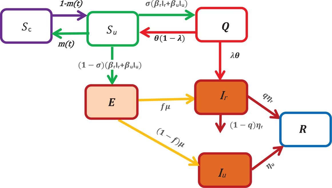
Fig. 1. A schematic of the model for COVID-19 transmission. In this figure, S u represents the number of unconfined susceptible, S c denotes the number of confined susceptible, E depicts the number of exposed, I r denotes the number of reported infectious, I u represents the number of unreported infectious or silent carriers, R denotes the number of recovered and Q denotes the number of quarantined. The arrow shows the people moving between the compartments.
In this paper, the unreported infectious individuals depict mainly the individuals with no clinical symptoms (asymptomatic or silent carriers) during their infectious period. They also include some infectious individuals with mild symptoms who thus often go unrecognised.
In what follows, we assume that these individuals don't die of the disease, while the reported infectious can die of disease at a rate (1 − q)η r where 1 − q is the fraction of reported individuals that die, q is the fraction of reported individuals that recover and 1/η r is the average length of infectious period of reported individuals (see Fig. 1).
An individual moves to the susceptible unconfined class, S u, either from the confined class at a rate 1 − m(t) or from the quarantined class at a constant rate θ(1 − λ). The fundamental parameter that we have introduced in our model to study the containment measures is the parameter m(t), it can be interpreted as the fraction of confined susceptible individuals at any time t. When the susceptible individuals are exposed to the virus, then the exposition provides either the reported class, I r or the unreported class, I u. Without making any distinction about the origin of the infection, we assume that a fraction σ of susceptible unconfined individuals which has been in contact with an infectious individual is quarantined with contact tracing while the other fraction (1 − σ) who was not detected by the contact tracing move to the exposed class E once effectively infected or stay in compartment S u otherwise. Then, the quantities (1 − σ)(β rI r + β uI u)S and σ(β rI r + β uI u)S represent the inflow of new individuals into the exposed class E and quarantined class Q respectively. The parameters β r and β u are the transmission rate of reported and unreported cases, respectively. We assume that reported individuals will participate in the infections with a lower rate than those unreported because they are generally isolated at the hospital or at home. However, they can transmit the infection to caregivers or their entourage. Moreover, they may have first been asymptomatic carriers contributing to the transmission of the virus. To simplify the notation, we set β u = β and β r = ñβ u = ñβ where ñ ∈ [0, 1]. The parameter ñ represents the infectivity of the reported cases and for ñ = 1, the reported and unreported have the same level of infectivity. Among the quarantined individuals, a fraction λ of individuals are effectively infected and moves in the reported infectious class, I r, after an average duration of isolation, 1/θ, and a fraction 1 − λ returns to the susceptible class without being reported infectious. We assume that only a fraction f of the individuals of exposed class becomes reported infectious and enters to the class I r at a rate μ where 1/μ represents the average length of the exposed period while the other fraction (1 − f) moves to the infectious unreported infectious class I u at a rate μ.
With the above considerations, the model describing the spread of COVID-19 takes the form:
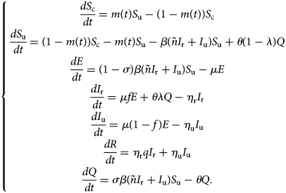
This model (1) is supplemented together with initial data S c(τ 0), S u(τ 0), E(τ 0), I r(τ 0), I u(τ 0), R(τ 0) and Q(τ 0).
Let DIr(t), DIu(t), CIr(t) and CIu(t) denote the daily number of reported cases, unreported one, the cumulative number of reported cases and unreported cases respectively at any time t. These quantities are obtained by solving the following equations:
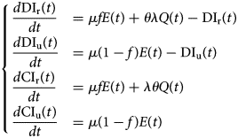
with initial conditions DIr(τ 0), DIu(τ 0), CIr(τ 0) and CIu(τ 0).
Basic reproduction number
The fundamental key concept in epidemiology is the basic reproduction number. Commonly denoted by ${\cal R}_0\comma \;$ it is the expected number of secondary cases produced by a typical infective individual introduced into a completely susceptible population, in the absence of any control measure [Reference Diekmann, Heesterbeek and Metz10, Reference van den Driessche and Watmough11]. Mathematically, ${\cal R}_0$
 is the spectral radius of the next-generation matrix. The next-generation matrix can be obtained by construction (cf. for instance [Reference Arino, Ducrot and Zongo12–Reference Hyman and Li14]). Using the method developed in [Reference van den Driessche and Watmough11], we obtain explicit formula for ${\cal R}_0$
 as follows:
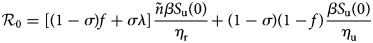
where β u = β and β r = ñβ. In the Appendix we give some details about the derivation of ${\cal R}_0.$
The quantity ${\cal R}_{\rm r}: = \lsqb {\lpar {1-\sigma } \rpar f + \sigma \lambda } \rsqb ñ \beta S_{\rm u}\lpar 0 \rpar /\eta _{\rm r}$ represents the average number of secondary infections produced by one reported infective individual during its infectious period, 1/η r; ${\cal R}_{\rm u}: = \lpar {1-\sigma } \rpar \lpar {1-f} \rpar \beta S_{\rm u}\lpar 0 \rpar /\eta _{\rm u}$
 represents the average number of secondary infections produced by one unreported infective individual during its infectious period, 1/η u.
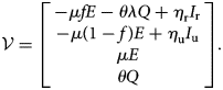
To take into account the containment measures, the large-scale testing, the social distancing and wearing masks measures, some constant parameters such as f, σ, β and S u(0) will be replaced in Equation (3) with the aforementioned time-dependent parameters. In this case, we can define the effective daily reproduction number, ${\cal R}_0\lpar t \rpar$ which measures the number of new infections produced by a single infected individual per day. This quantity is obtained by solving the following equation:
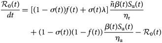
with initial condition ${\cal R}_0\lpar 0 \rpar = {\cal R}_0$ defined in Equation (3).
Construction of the containment rate
To analyse the effectiveness of containment measures, we assume that a fraction m(t) of susceptible individuals in the population is confined at any time t. Furthermore, we introduce a parameter p which indicates the maximum percentage of the population that the government confines. This fraction should be greater than the quantity $1-1/{\cal R}_0$ to be sure of its effectiveness [Reference Ducrot13, Reference Zongo, Dorville and Gouba15]. This parameter varies from country to country and can be set in advance for a given country. Let τ 0 denotes the starting date of epidemic, τ 1 represents the date at which a government decides to apply the containment measures, τ 2 denotes the date at which a fraction p of the population is confined, τ 3 stands for the date at which the government decides to exit progressively the containment measures because either the restrictions take effect or there are budget or social limitations and τ f denotes the date for the end of the containment measures. Now, we divide the containment rate m(t) into four phases:
Phase 0: period without containment measures (from date τ 0 to τ 1), then m(t) = 0.
Phase 1: period when containment is taking place until the government reaches its maximum containment effort (from date τ 1 to τ 2). In this phase we assume that the function m increases exponentially and reach the value p at date τ 2. It follows that m takes the form m(t) = 1 − exp ( − a(t − τ 1)) where a = −ln(1 − p)/(τ 2 − τ 1).
Phase 2: period where the maximum effort is maintained (from date τ 3 to τ 4) and m(t) = p.
Phase 3: period at which the government decides to relax the containment measures (from date τ 3 to τ f). This drop is linearly depending on the time so that the value of m at date τ f equals to 0. Then m is described as follows: m(t) = p + b(t − τ 3), where b = −p/(τ f − τ 3).
Model parameters
Before to go further, let us point out that in our paper, the values of the parameters f, σ, μ, θ, τ 0, τ 3, τ f, as well as the initial values S u(τ 0), S c(τ 0) and I r(τ 0) were chosen from expert opinions. The values of the parameters τ 2, λ, ñ, p, β, σ, η r, η u as well as the initial values CI u(τ 0), Q(τ 0) and E(τ 0) were unknown. However, it is possible to identify them from specific time data. The value of the parameter q can be easily computed from current data. By setting x = (τ 2, λ, ñ, p, β, σ, η r, η u, I u(τ 0), Q(τ 0), E(τ 0), τ 2), we estimated an optimal value of x that fit with the data from France by minimising the following error function:
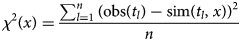
where n is the number of observed data, obs(t l) and sim(t l, x) are the observed and calculated data at time t l respectively.
Chosen values: f, σ, μ, θ, τ0, τ3, τf, Su(τ0), Sc(τ0) and Ir(τ0)
Initial conditions: We started the simulations at the moment where in France, the number of reported cases were identified with 12 individuals, i.e. precisely on the date τ 0 = 25 February. Then I r(τ 0) = 12. The population of France is around 66 999 000 inhabitants [16], thus, we set S c(τ 0) =66 999 000. At that date, there were no confined individuals, thus S c(τ 0) = 0.
Value of parameter f: Recall that, (1 − f) stands for the fraction of exposed individuals that becomes unreported infectious and corresponds to the proportion of asymptomatic or silent carriers or mild infectious. (1 − f) ranges from 17.9% to 86% [1, Reference Daniel17–Reference Kenji20] and some reviews therein [Reference Zhao21]. The fractions of unreported individuals in these previous studies are derived from the number of tests performed. Therefore, the current fraction may be seriously underestimated. During the onset of COVID-19 in France, there were very little screening tests. That's why, we estimated that 1 − f = 0.8 (i.e. f = 0.2). Furthermore, we make it vary in the scenario 3 (effectiveness of the large-scale testing), as soon as the number of tests increases.
Value of parameter σ: The value of parameter σ was calibrated to 0.2 so that σ = f. In scenario 3, we assume that f increases in the same order as σ when the time evolves (see Fig. 2(c)), because when the number of tests increases, the fraction of reported cases increases and thus the fraction σ of susceptible unconfined individuals that is quarantined increases with contact tracing.
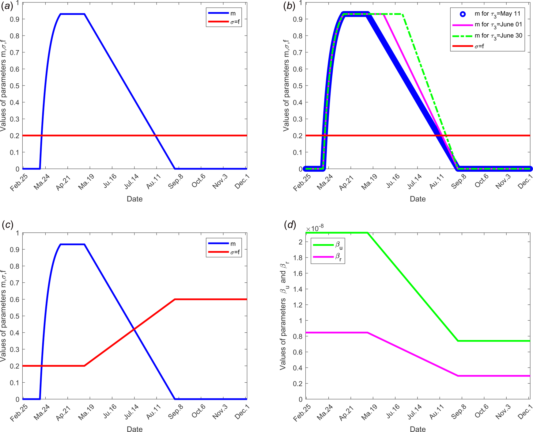
Fig. 2. Evolution over time of parameters m, σ, f, β r, β u and τ 3 according to each scenario; the other parameters of the model are fixed as shown in Table 1: (a) for scenario 1, only the parameter m is time dependent, f = σ = 0.2, β r = 0.846 × 10⁻⁸, β u = 2.115 × 10⁻⁸ and τ 3 = 11 May for all time. (b) For scenario 2, f = σ = 0.2, β r = 0.846 × 10⁻⁸, β u = 2.115 × 10⁻⁸ for all time, only the parameter m is time dependent for three different values of the date at which the containment measures are relaxed, τ 3, more precisely when τ 3 takes the values 11 May, 01 and 30 June. (c) For scenario 3, we set τ 3 =May 11, m, f and σ evolve over time, β r = 0.846 × 10⁻⁸, β u = 2.115 × 10⁻⁸. (d) For scenario 4, τ 3 =11 May, f = σ = 0.2, m evolves as in (a), in addition, the transmission rate β r and β u evolve. (e) For scenario 5, τ 3 = 11 May, f, σ, m evolve as in (c), moreover β r and β u evolve as in (d).
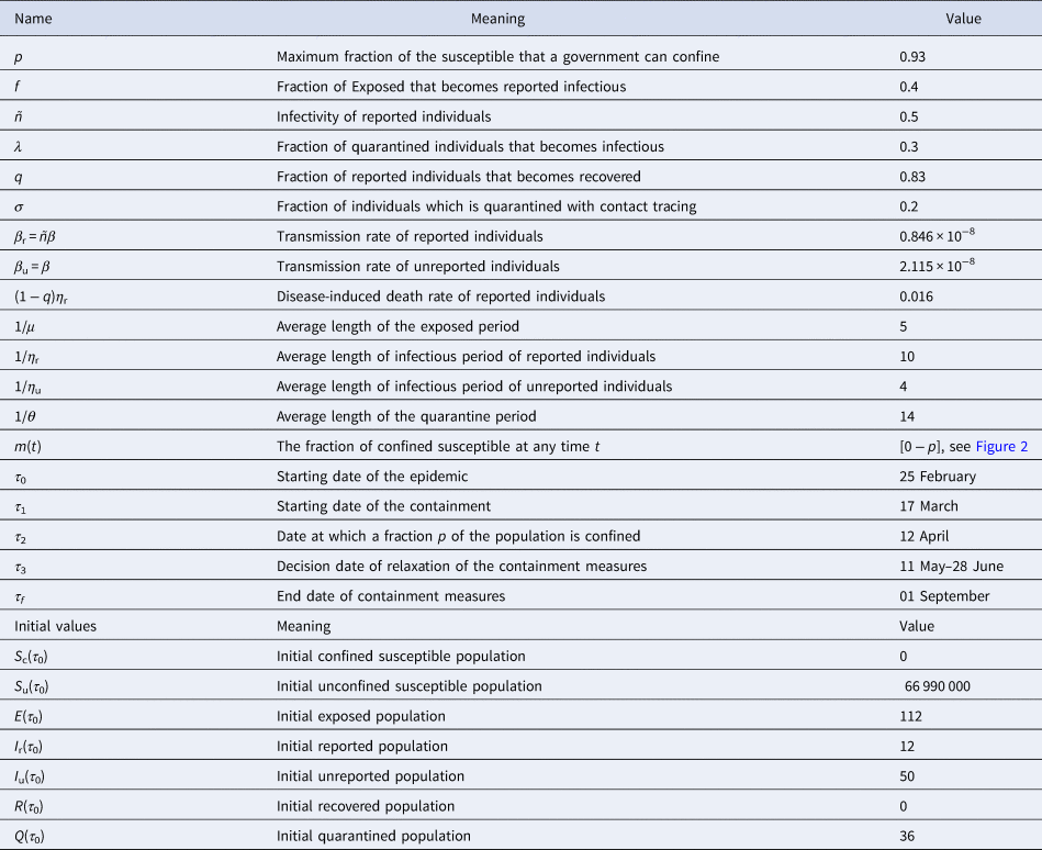
Table 1. List of parameters and their meaning and the parameter ranges for which the model was solved
Value of parameter τ 1: The starting date of the containment was fixed on 17 March, then τ 1 = 17 March.
Value of parameter τ 3: According to the announcement of French government of 13 April, a gradual deconfinement started on 11 May. So for model validation, we fixed τ 3 = 11 May.
Value of parameter τ f: We fixed the end date of containment measures on 1 September.
Value of parameter μ: The mean incubation period 1/μ was fixed to 5 days see [1, Reference Lessler22, Reference Backer, Klinkenberg and Wallinga23].
Value of parameter θ: We considered 14 days to isolate the quarantined individuals, therefore, 1/θ = 14 days.
Estimated values: τ2, λ, ñ, p, β, σ, ηr, ηu, Iu(τ0), Q(τ0), E(τ0), τ2 and q
By calibrating the model with the data corresponding to the cumulated reported cases for France, we identified some values of model parameters giving a good fit of the observed data obtained in [24]. The parameter values and initial conditions estimated are listed in Table 1.
Value of parameters τ 2and p: We estimate that the government has successfully confined 93% of the population on the date 12 April, thus, τ 2 = 12 April and p = 0.93. This value means that 93% of the population was confined on date τ 2 equals to 12 April, thus S c(τ 2) = 62 300 700. In this case, 7% of the population that remained active and we set S u(τ 2) = 4 689 300. Note that this number corresponds to approximately 15.78% of active population in France which was 29 700 000 according to INSEE in 2017 [25].
Value of parameters η rand η u: By fitting with data from France, we estimate that the mean duration of infectious period for unreported individuals, 1/η u = 4 days and for reported ones, 1/η r = 10 days.
Value of parameters β r, β uand ñ: We estimated that the infectivity of reported cases ñ equals to 0.40 compared to infectivity of unreported which is 1. The transmission rate β u = β of unreported individuals is estimated to 2.115 × 10⁻⁸/day, then the transmission rate of reported individuals equals to β r = βñ = 0.846 × 10⁻⁸/day.
Value of parameter q: Since 1 − q represents the fraction of reported individuals that dies, thus ${{1-q} = {{{\rm Cumulative\;number\;of\;death\;among\;the\;reported\;individuals}} \over {{\rm Cumulative\;number\;of\;reported\;individuals}}}.}$
From current data (31 July), we find 1 − q = 30 254/186 573 = 0.1622. It follows that the disease-induced death rate of reported individuals, (1 − q)η r, equals to 0.1622 × 1/10 = 0.0162/day. Furthermore, the fraction of reported individuals that becomes recovered equals to q = 0.8378.
Value of parameters E(τ 0), Q(τ 0) and I u(τ 0): We estimate that at date τ 0, we have Q(τ 0) = 36, I u(τ 0) = 50 and E(τ 0) = 112.
Simulation experiments: application to data from France
Scenario 1: validation of model with data from France
We selected for model validation, the data obtained for daily reported (DRIr) and cumulative reported (CRIr) cases for France see [24]. Some constants and parameters involved in the model are listed in Table 1. The results of this scenario are illustrated in Figure 3.
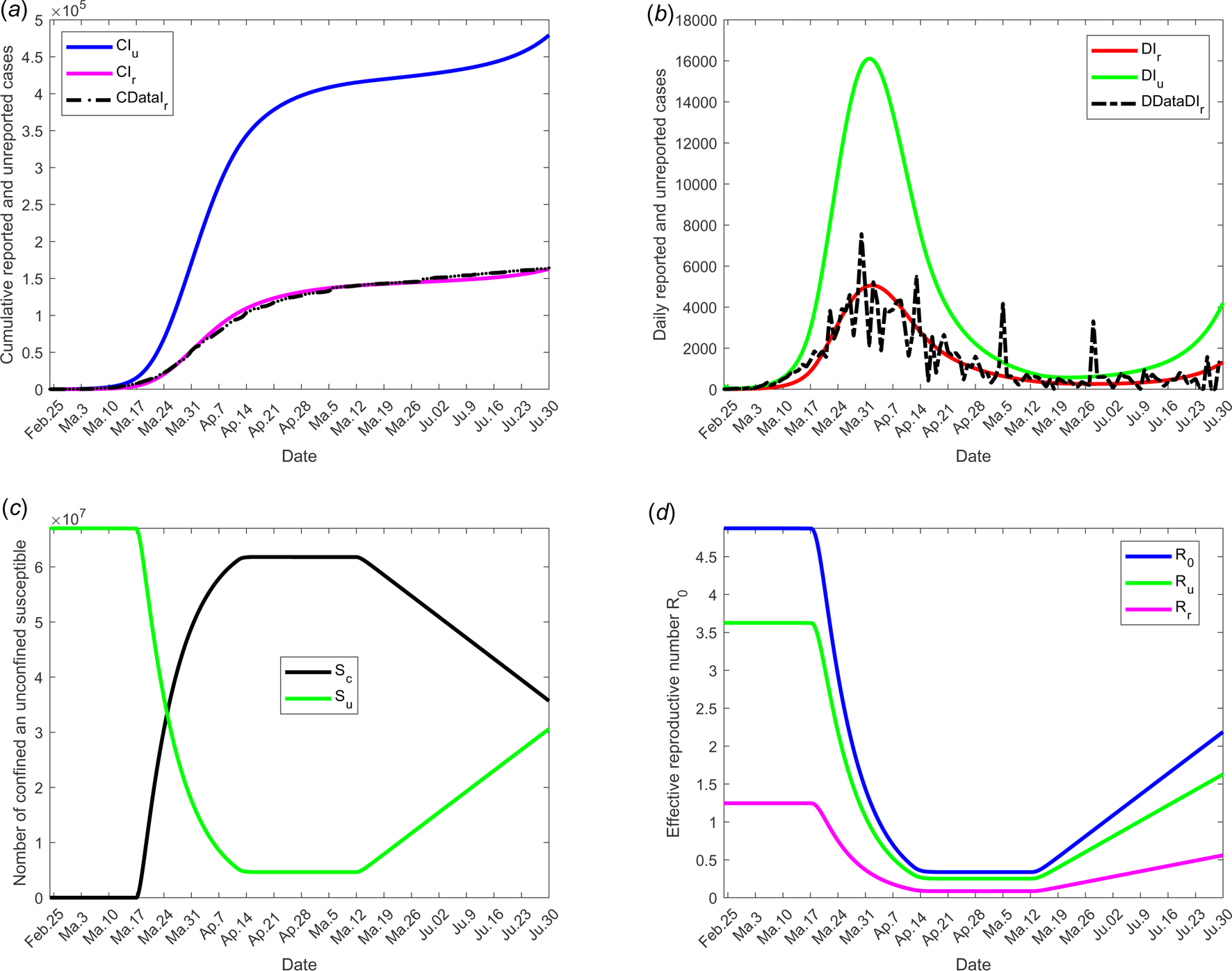
Fig. 3. Scenario 1: Validation of model with currently data from France. The date at which the containment measures are relaxed, τ 3, was fixed to 11 May; the end date of containment measures, τ f, was fixed to 1 September. (a) The cumulative number of reported CIr and unreported CIu cases simulated, and observed data CIrData. (b) The daily number of reported DIr and unreported DIu cases from the model and observed data DDataIr. (c) The confined and unconfined susceptible S c and S u. (d) The daily reproductive number ${\cal R}_0$ . In this scenario, the values of the parameters were estimated and listed in Table 1 except for the containment function m which varies between 0 and 1 (see Fig. 2(a)).
Scenario 2: effectiveness of containment measures
The objective of this scenario is to analyse if the outbreak might stop for different values of the date at which the containment measures are relaxed, namely τ 3. Then, the value of the latter is assumed varying from 11 May, 1 and 30 June. The end date of containment measures τ f, is fixed to 1 September. The values of the parameters used are listed in Table 1 except for the containment function m that varies (see Fig. 2(b)).
The results of this scenario are illustrated in Figure 4.
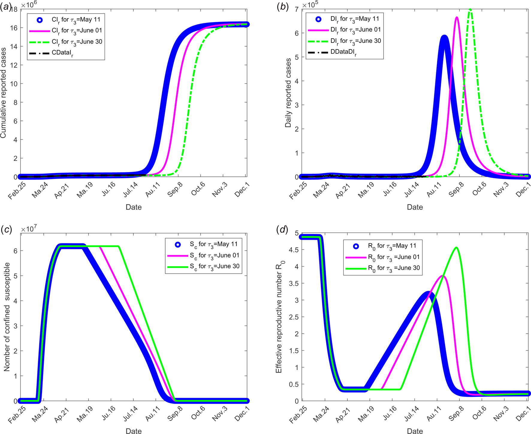
Fig. 4. Scenario 2: Longer-term forecasting of epidemic spreading according to different values of the date at which the containment measures are relaxed, τ 3 that varies between 11 May and 01 and 30 June. The end date of containment measures τ f was fixed to 1 September. (a) The cumulative number of reported CIr cases simulated. (b) The daily number of reported DIr cases from the model. (c) The number of confined susceptible S c. (d) The daily (effective) reproductive number ${\cal R}_0$ . In this scenario, the values of the parameters were estimated and listed in Table 1 except for the containment function m which varies between 0 and 1 for different values of τ 3 (see Fig. 2(b)).
Scenario 3: effectiveness of the large-scale testing
To investigate the effectiveness of the large-scale test of detection of infected individuals, the date at which the containment measures are relaxed, τ 3, is fixed to 11 May; the end date of containment measures, τ f, is fixed to 1 September. We assume that between the dates τ 3 and τ f, the fraction of reported cases f increases linearly and reach 200% of its initial value and the fraction of susceptible individuals which is quarantined σ is also increased linearly to reach 200% of its initial value (see Fig. 2(c)), the initial values is estimated in scenario 1. The values of the other parameters are listed in Table 1 except for the containment function m that varies (see Fig. 2(b)).
The results of this scenario are illustrated in Figure 5.
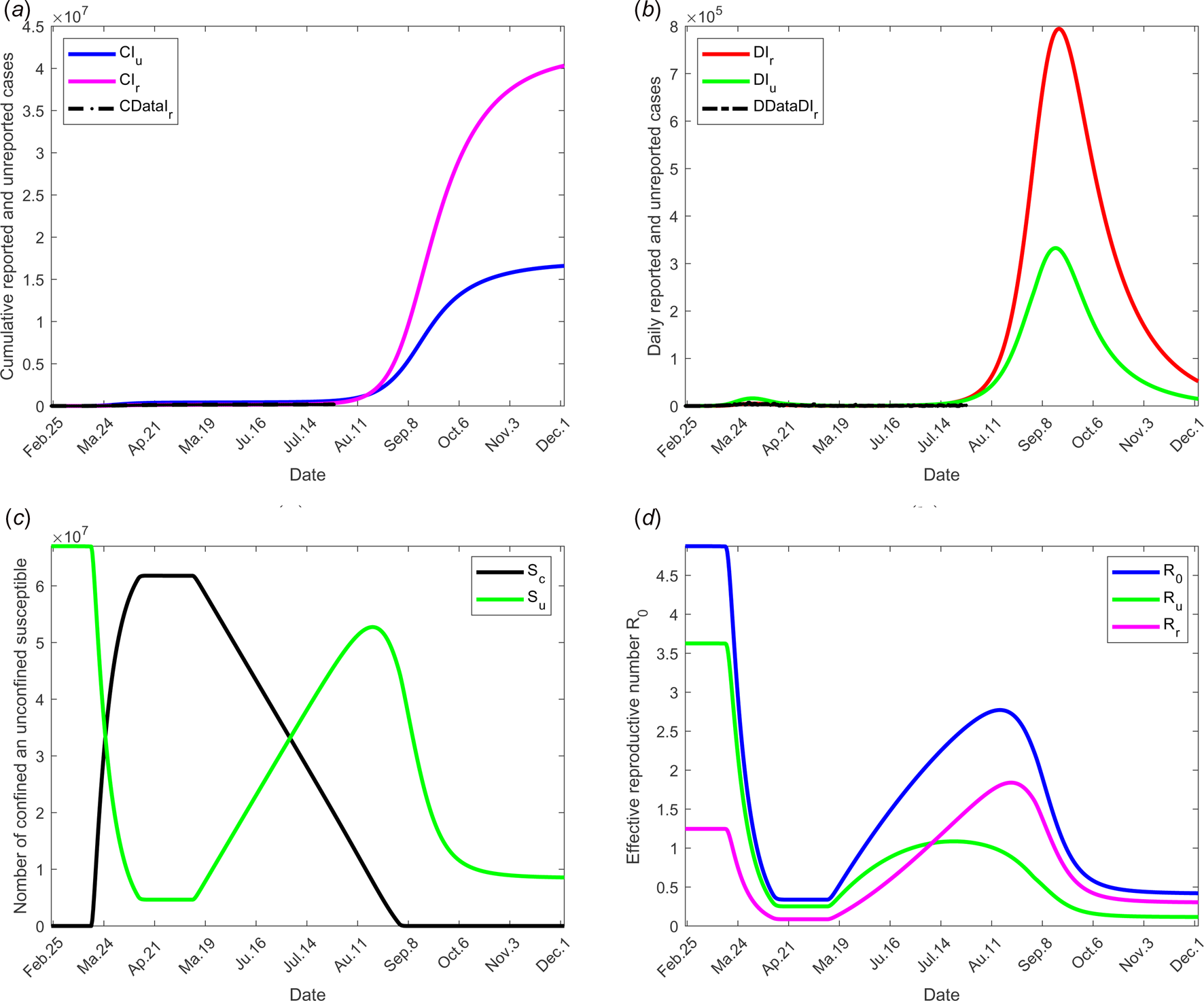
Fig. 5. Scenario 3: Longer-term forecasting of epidemic spreading in case of large-scale tests of detection on infected individuals. τ 3 was fixed to 11 May; τ f was fixed to 01 September. Between the dates τ 3 and τ f, the parameter f was assumed to increase linearly to reach 200% of its initial value, σ increased linearly to reach 200% of its initial value (see Fig. 2(c)). The values of the other parameters are listed in Table 1 except for m that varies (see Fig. 2(b)). (a) The cumulative number of simulated reported CIr and unreported CIu cases and observed data CIrData. (b) The daily number of simulated reported DIr and unreported DIu cases and observed data DDataIr. (c) The number of simulated confined and unconfined susceptible S c and S u. (d) The daily reproductive number ${\cal R}_0$ .
.
Scenario 4: social distancing and/or wearing masks measures
To study the social distancing and/or wearing masks measures, the date at which the containment measures are relaxed, τ 3, was fixed to 11 May; the end date of containment measures, τ f, is fixed to 1 September. We assume that between the dates τ 3, and τ f, the transmission rate β decreases linearly to reach 75% of its initial value (see Fig. 2(d)). The values of the other parameters are listed in Table 1 except for the containment function m that varies (see Fig. 2(b)).
The results of this scenario are illustrated in Figure 6.
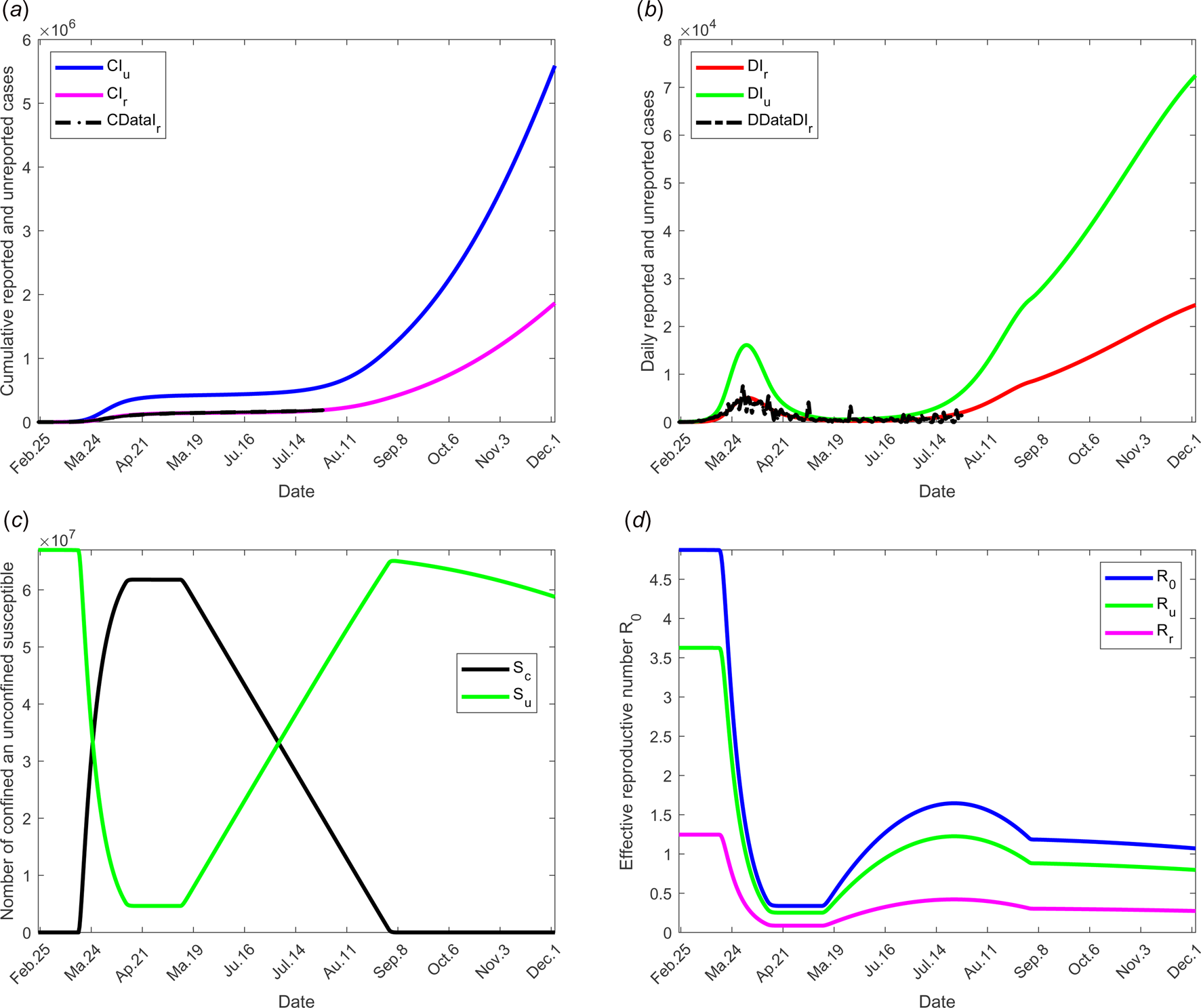
Fig. 6. Scenario 4: Longer-term forecasting of epidemic spreading in case of the social distancing and wearing masks measures. τ 3 was fixed to 11 May; τ f was fixed to 01 September. Between the dates τ 3 and τ f, the parameter β decreases of 75% of its initial value (see Fig. 2(d)). The values of the other parameters are listed in Table 1 except for m that varies (see Fig. 2(b)). (a) The cumulative number of simulated reported CIr and unreported CIu cases and observed data CIrData. (b) The daily number of simulated reported DIr and unreported DIu cases and observed data DDataIr. (c) The number of simulated confined and unconfined susceptible S c and S u. (d) The daily reproductive number ${\cal R}_0$ .
.
Scenario 5: combined effects of large-scale testing and social distancing measures
To test the combined effects of large-scale testing and social distancing social and/or wearing masks measures, we combine the conditions of scenarios 1 and 2. The date at which the containment measures are relaxed, τ 3, is fixed to 11 May; the end date of containment measures, τ f, is fixed to 1 September. Between the dates τ 3 and τ f, we assume that f increases linearly to reach 200% of its initial value, σ increases linearly to reach 200% of its initial value and β decreases of 75% of its initial value see Figure 2(d) for these different variations of parameter values.
The results of this scenario are illustrated in Figure 7.
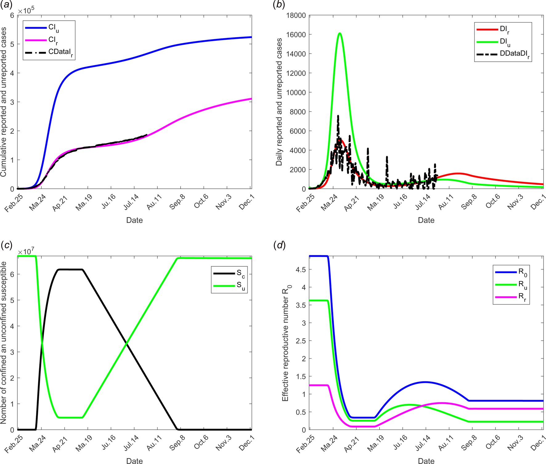
Fig. 7. Scenario 5: Longer-term forecasting of epidemic spreading in case of both social distancing and/or wearing masks and large-scale tests. τ 3 was fixed to 11 May; τ f was fixed to 1 September. Between the dates τ 3 and τ f, the parameter f increases linearly to reach 200% of its initial value, σ increases linearly to reach 200% of its initial value (see Fig. 2(c)). β decreases to 75% of its initial value (see Fig. 2(d)). The values of the other parameters are listed in Table 1 except for m that varies (see Fig. 2(b)). (a) The cumulative number of simulated reported CIr and unreported CIu cases and observed data CIrData. (b) The daily number of simulated reported DIr and unreported DIu cases and observed data DDataIr. (c) The number of simulated confined and unconfined susceptible S c and S u. (d) The daily reproductive number ${\cal R}_0$ .
.
Discussion and conclusion
This model takes into account the measures of confinement, distinguishing between confined individuals, quarantined individuals and isolated individuals. Many values were estimated to fit the beginning of expansion of disease in France, other were inferred from expert opinions, see Section ‘Model parameters’. The proportion (1 − f) ranges from 17.9% to 86% [1, Reference Daniel17–Reference Kenji20] and some reviews therein [Reference Zhao21]. The lower value was observed on board of the Diamond princess, i.e. in conditions which are not representative of large-scale populations living in larger surfaces. On the other hand, in [Reference Li26] and in a WHO report, it was estimated that between 80% and 86% of all infections were undocumented. Since this fraction is dependent on the number of tests performed and since during the onset of COVID-19 in France, there were fewer screening tests, we eventually chose f = 0.2.
As for f, the mean duration of infectious period is a debatable point. In [Reference Saurabh27], the authors estimate that the asymptomatic individuals had median virus persistence duration of 8.87 days (95% confidence interval 7.65–10.27). This duration varies also between asymptomatic and symptomatic individuals [Reference Zhang28], even when mildly affected. By contrast, all severe cases were still tested positive at or beyond day 10 post-onset [Reference Yang29]. This longer virus persistence in severe cases as compared to milder cases has been also demonstrated by [Reference Sun30] but not by all authors, see some reviews therein [Reference Zhao21]. Note also that in the literature, the estimate of the mean duration of infectious period of reported individuals is not always clear, since some authors include hospitalisation or isolation period, others do not. Results vary between 2 and 8 days [Reference Li26, Reference Chinazzi31, Reference Kucharski32]. Our model implicitly takes into account a combined effect of duration of infectivity and viral load, which results in risk of transmission. Indeed, the mean duration of infectious period estimated to be 10 days for reported individuals is coherent with the estimation in [Reference Ong33] based on clinical, microbiologic, epidemiologic and clinical data. Since we estimate the infectivity of the reported cases to be equal to 0.4, that of unreported cases in term of duration of infectious period, it means that reported individuals are infectious for 40% of their infectious period, i.e. 4 days. If the infectivity is interpreted in terms of viral load, it means that 40% of the viral load excreted by the infectious reported cases is infective. Such a link between duration of infectious period and infectivity (i.e. interpreted in terms of viral load) also holds in the literature except in [Reference Zou34] where the authors observed no difference in viral load between asymptomatic and symptomatic patients. In [Reference Long35] the virus level in the asymptomatic group was significantly lower than that in the symptomatic group in the acute phase.
Figure 3 shows the adequacy of the model for predicting the evolution of number of cases in the beginning of the crisis until end of June. It also shows that as soon as confinement is reduced or stopped, the daily reproduction number ${\cal R}_0(t)$ value increases again and a new wave of epidemics is to be expected as soon as its value is higher than 1. As observed in Figure 4 (for longer-term forecasting), such waves are expected to appear very shortly after reduction of confinement, once the incubation period is spent. These values will allow predicting the effectiveness of the containment measures as well as risk and the intensity of possible resurgences of the new waves of epidemic in France. Indeed, the measures of confinement have a strong impact on the value of the daily reproduction number ${\cal R}_0(t).$
 Figure 4 shows that, while it was equal to nearly 5 in the beginning of the disease, before confinement, it decreased to about 0.5 as long as confinement of most people takes place and increased to a lower value, between 2 and 2.5, that is about half its former value. But even if its value is reduced, it remains higher than 1. It is also to note that, unexpectedly, its value was lower when end of confinement was earlier. Figures 3 and 4 show that the current increase in the number of cases could be expected as soon as containment was relaxed from mid-May to September. However, the number of cases are expected to decrease if a higher proportion of infected people are detected and confined, which is currently the case. Delaying the very starting date of deconfinement to 30 June would have resulted in a later and higher wave but not as late as could be expected for a starting date to 11 May. All French people are expected to be either reported or unreported infected individuals at the end of 2020, i.e. before expected development of vaccines. However, some of those values may change with evolution of measures of prevention such as social distancing and/or wearing masks, large-scale testing, treatment of the disease.
Social distancing and wearing masks measures directly influence the transmission rate which is expected to dramatically decrease with the increasing tendency to wear masks. Its effect was investigated in scenario 3 where the transmission rate was assumed to decrease linearly to reach the value 75% of its initial one as shown in Figure 2(d). The results of this scenario are shown in Figure 5. The transmission rate may be dramatically decreased. But the results show that this measure alone is insufficient to eliminate the disease.
The effectiveness of the large-scale test of detection of infected individuals was analysed and shown in Figure 6. The fraction of reported cases, from date τ 3 to τ f, the fraction of reported cases f was assumed increase linearly to reach the value 200% of its initial one and the fraction of susceptible individuals which is quarantined σ was also increased linearly to reach the value 200% of its initial one (see Figs 2(b) and (c)). These values may be observed by tracking all former contacts of any newly reported case, and systematically testing them. As in the former scenario dates of relaxation and end of containment measures were fixed to 11 May and 1 September respectively. Results show that this measure without further action is also insufficient to control the outbreak.
The combined measures of large-scale testing and social distancing and/or wearing masks measures was studied in scenario 5. The transmission rates (reported and unreported individuals) were assumed to decrease from 75% to date τ 2 to τ f (see Fig. 2(d)). Figure 7 shows the effectiveness of these combined measures and the potential of such a strategy. In particular, it shows that predicted data are compatible with the current situation with no evidence yet of a second wave. This result also shows that protective measures must be maintained for a long term before the hypothesis of a second wave may be discarded.
In the absence of any control measure, the basic reproduction number ${\cal R}_0$ is equal to 4.8739. Most of this value is due to the weight of transmission by unreported individuals $\lpar {\cal R}_{\rm u} = 3.6271\rpar$
 and the weight of transmission by reported cases accounts for much less $\lpar {\cal R}_{\rm r} = 1.2468\rpar$
 . These values show that the major number of secondary infections is produced by the unreported individuals. With increasing use of appropriate tests, reported individuals will be more precisely diagnosed, thus the fraction of reported cases f will increase and thus the importance of ${\cal R}_{\rm r}$
 in the total value of ${\cal R}_0$
 . Since the infectivity of reported individuals was estimated at 0.4 compared to infectivity of unreported the increase in ${\cal R}_{\rm r}$
 will be very small showing the importance of detecting infectious individuals; the evolution over time of the effective reproductive number ${\cal R}_0\lpar t \rpar$
 and effective weight of transmission ${\cal R}_{\rm r}\lpar t \rpar$
 and ${\cal R}_{\rm u}\lpar t \rpar$
 are shown in Figure 7(d). Therefore, the reported individuals will have a lower propensity to transmit the virus. Through stronger measures of prevention, the probability of contaminating other people will be lower.
With the confinement measures, the minimal percentage (critical fraction) of susceptible individuals that should be confined to eliminate the COVID-19 equals to $1-1/{\cal R}_0$ (see for instance [Reference Ducrot13, Reference Zongo, Dorville and Gouba15]). By confining more susceptible individuals, we increase the kinetics of elimination of the disease. By fitting the model with the French data, we estimated this fraction to p = 93%. This value belongs to the critical interval, namely $\rsqb 1-1/{\cal R}_0\comma \;1\rsqb \simeq \rsqb 0.8\comma \;1\rsqb .$
By analysing the results of simulations, we can conclude that the containment measures appear to have slowed the growth of the COVID-19 outbreak. Our model predicts that a second big wave of the epidemic may not be avoided if the situation remains unchanged and if the French government does not maintain the current efforts on large-scale tests, obligation of wearing masks inside and in some cases outside and other prophylactic measures. However, it also shows that these measures are efficient to avoid such a risk, thus preserving public health and avoiding a new confinement and all its terrible consequences, see Figures 3 and 4. While if no measures were implemented, even only one infected individual in the population would result in a new wave of infections and a new period of confinement. Some obligations will succeed in avoiding a second wave of COVID-19.
In this paper, we formulated a new model to describe the spread of COVID-19 to understand the effectiveness of the containment and quarantine measures. It is able to reproduce observed data from France and probably other countries.
Acknowledgement
The authors would like to thank two anonymous referees for many helpful suggestions.
Conflict of interest
None.
Data availability statement
The datasets generated during the current study are graphical represented in the scenarios 1-5. The datasets from France used to fit the model during the current study are freely available via online public domains [25].
Appendix
Some details about the derivation of ${\cal R}_0$

In order to define ${\cal R}_0\comma \;$ for model (1), we begin to find the disease-free equilibrium point by letting the compartments S c, Q, E, I r, I u, and R be zero and S u = S u(0).
Let ${\cal F}\lpar {I_{\rm r}\comma \;I_{\rm u}\comma \;E\comma \;Q} \rpar$ denotes the inflow of new individuals into the infected classes I r, I u, E and Q

and ${\cal V}\lpar {I_{\rm r}\comma \;I_{\rm u}\comma \;E\comma \;Q} \rpar$ denotes all other flows within and out of the infected classes,
Let $F = D{\cal F}$ and $V = D{\cal V}$
 be the Jacobian matrices of the maps ${\cal V}$
 and ${\cal F}$
 , respectively, evaluated at the disease free equilibrium:
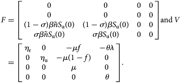
A straightforward computation shows that
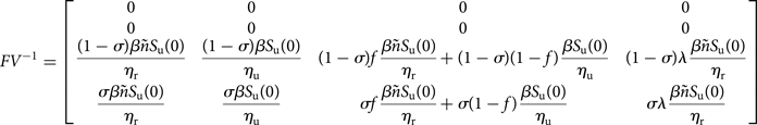
Following [Reference van den Driessche and Watmough11], the matrix FV −1 is well defined, and is the next-generation matrix and ${\cal R}_0$ is the spectral radius of FV −1.


 Open access