Article Information

Hiroshi Furutani^1*, Tomoyuki Hiroyasu^1,2

¹AI x Humanity Research Center, Doshisha University, Kyotanabe City, 6100394, Kyoto, Japan

²Department of Biomedical Information, Doshisha University, Kyotanabe City, 6100394, Kyoto, Japan

*Corresponding author: Hiroshi Furutani, AI x Humanity Research Center, Doshisha University, Kyotanabe City, 6100394, Kyoto, Japan.

Received: 08 September 2022; Accepted: 14 September 2022; Published: 20 September 2022

Citation: Hiroshi Furutani, Tomoyuki Hiroyasu. Estimation of COVID-19 Cases in Japanese Prefectures Using a Gumbel Distribution. Archives of Clinical and Biomedical Research 6 (2022): 756-763.

Abstract

Keywords

COVID-19; Extreme Value Theory; Estimation; Gumbel Model; Infection in Japan

Article Details

1. Introduction

Various mathematical models have been developed for capturing the spreading process of infectious diseases. Among these models, the basic Kermack- McKendrick model is a popular theory [1]. As a simple example, Kermack and McKendrick presented a compartment model, usually referred to as a susceptible, infected, recovered/removed (SIR) model [2, 3]. After some manipulation of the SIR model, we can derive the logistic growth model, which has been used in epidemiology as a standard method [4, 5]. In addition, many studies using an extended form of compartment models have been reported [6]. From the first wave of a pandemic in many regions, the daily plot of reported infections is single-peaked and skewed to the right. Time-series data in general have three phases:

• A. an exponential increase in the early stage,
• B. a change from increasing to decreasing in the intermediate stage, and
• C. a slowly decreasing final stage.

Although distributions of the exponential family have a simple form, many studies have suggested that the exponential distribution can reasonably reproduce the data in the decreasing phase [7]. Applications of the EVT are relatively new in the mathematical modeling of epidemiology and are used for forecasting the outbreak of pathogenic influenza [8] and for analyzing spreading of SARS and COVID-19 [9]. However, the EVT has been widely used to analyze rarely occurring events in many applications [10, 11] such as reliability engineering [12] and mortality analysis [13]. In the EVT, there are three classes of distributions, which are widely known as Gumbel, Fr´echet, and Weibull families [11, 14]. There are two types of Gumbel functions: the Gumbel function for maximum values and the Gum- bel function for minimum values. The present study uses the Gumbel function for maximum values, which is simply referred to as the Gumbel function. The Gumbel function has been used for analyzing COVID-19 time-series data in [15] and [16]. The Gumbel cumulative distribution function is given as

F_G(t) = exp{−e^−y(t)},                                             y(t) = a(t − b),                                 (1)

where a and b are parameters that decide the shape (a) and position (b), respectively, of the distribution [17]. The parameter b corresponds to the position of the node. We can find applications of the Gumbel distribution in the literature of evolutionary computation [18]. In some optimization problems, the number of steps necessary to obtain an optimum solution can be expressed by a Gumbel distribution [19], the mathematical derivation of which is given in [20]. As of March 31, 2022, Japan had recorded a total of 6, 565 k confirmed cases of COVID-19, including 28, 128 deaths. From January 1, 2022 to March 31, 2022, the numbers of confirmed cases and deaths were 4, 831 k and 9, 731, which are 73.5% and 34.6% of the respective totals. The surge of infections during this period is usually referred to as the sixth wave of the outbreak in Japan. Japan is divided into 47 administrative divisions, known as prefectures. Its population was estimated at 126, 476 k people in 2020. In most prefectures, time-series data of daily cases during the sixth wave have a single-peaked and right-skewed form. In the present paper, we report the estimation of the daily number of infections during the sixth-wave outbreak in Japan and its constituent prefectures using a Gumbel distribution. We also analyze the nation-level daily number of deaths in Japan.

2. Preliminaries

Among the 47 Japanese prefectures, we analyze 12 prefectures in three main cosmopolitan areas and four prefectures in other areas.

1. A.Tokyo metropolitan area: Tokyo, Saitama, Chiba, and Kanagawa
2. Osaka metropolitan area: Osaka, Kyoto, Hyogo, and Wakayama
3. Nagoya metropolitan area: Aichi, Gifu, Mie, and Shizuoka
4. Other areas: Hokkaido, Tochigi, Toyama, and Nagasaki

The total population of these prefectures is approximately 62.7% of the Japanese population. The present study uses the dataset of NHK, a Japanese government- owned public broadcaster. We downloaded two files from the website of NHK on April 4, 2022: nhk-news-covid19-domestic-daily-data.csv and nhk-news- covid19-prefectures-daily-data.csv. https://www3.nhk.or.jp/news/special/coronavirus/data-all and data.

The dataset contains daily numbers of COVID-19 infections and deaths from January, 2020 to April 3, 2022. Three daily numbers for April 2022 are used for the smoothing process of moving average.

3. Methods

The present paper uses the following notation: U_t indicates the cumulative numbers of infections or deaths on the t-th day, and u_t indicates the daily count of infections or deaths on the t-th day. Since reported data of daily counts usually fluctuate around trend curves, we use a seven-day moving average

m_t = {u_t−3 + . . . + u_t + . . . + u_t+3}/7.

Using the relation ln F_G(t) = −e^−y(t), the probability density function for the Gumbel distribution f_G(t) is given by

f_G(t) = ae^−y(t) F_G(t). (2)

In order to estimate U_t and m_t, it is necessary to know the total number N, and

U_t ≈ N F_G(t), m_t ≈ N f_G(t). (3)

This method uses the value M_t defined as

and M_t can be approximated by

Thus, we have

Mt ≈ ae−a(t−b)

We can obtain M_t from the reported daily numbers. The final task is to estimate the parameters in y(t) = a(t − b).

Applying a logarithmic transformation, we define L_t as

L_t = − ln M_t ≈ − ln a + a(t − b) = at + {− ln a − ab}. (6)

Thus, L_t may be approximated by a linear function of t as

L_t ≈ q₀ + q₁t,

and coefficients q₀ and q₁ can be obtained by the linear regression method. From these values, we have estimates of the Gumbel parameters,

a = q₁, b = −(ln q₁ + q₀)/q₁. (7)

The regression analysis uses two sets T and Y having 12 elements

T = {ts, ts + 1, . . . , te},

where ts and te denote the starting time and ending time, respectively, of the regression with te = ts + 11, and

Y = {L_ts, L_ts+1, . . . , L_te}.

The next step is an estimation of the total number N_e. We use the average of the ratio

Then, the estimate of U_t is given by

U_e(t) = N_e F_G(t);

and we use U_e(t) for the estimation of daily number n_e(t)

4. Results

This analysis uses daily numbers in Japan from September 1, 2021 to April 3, 2022, and presents estimated daily numbers from January 6, 2022 (t = -25) to March 31, 2022 (t = 59).

4.1 Infections and Deaths in Japan

First, we consider the number of daily infections and deaths of Japan during the sixth outbreak. Table 1 presents the time windows for the regression analysis and the obtained model parameters: Ne, a, and b. Theories 1 and 2 indicate infection numbers, and Theories 3 and 4 indicate deaths.

Table 1: Daily number of infections and deaths in Japan.

Window for regression analysis and estimated model parameters. Theories 1 and 2: infections. Theories 3 and 4: deaths.

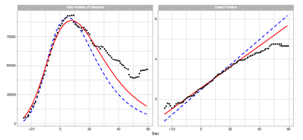
Figure 1 shows a comparison of the reported daily number of infections in Japan and the Gumbel model. Model estimations for the time course of the sixth outbreak are carried out with two different time windows for the regression analysis. The left-hand panel shows the estimated daily numbers for Theories 1 and 2. Theory 1 uses a 12-day time window of 7 ≤ t ≤ 18, and Theory 2 uses 1 ≤ t ≤ 12. Theory 1 calculates the regression coefficients using the dates for six days later than those of Theory 2. We note that Theory 2 underestimates the reported data of t ≥ 15 in the region of decreasing phase. In contrast, Theory 1 can satisfactorily fit the data for t ≤ 25, and deviation from reported data is smaller than that for Theory 2 for almost all dates. The right-hand panel shows L_t and estimated linear lines q₀ + q₁t of Theories 1 and 2.

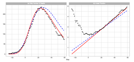
Figure 2 shows a comparison of the reported daily number of deaths and the Gumbel model estimation. The left-hand panel shows the estimated daily numbers for Theories 3 and 4, and right-hand panel shows L_t and two esti- mated linear lines q₀ + q₁t. As presented in right-hand panel, the window of [0, 12] cannot be used for the regression analysis. The estimation of Theory 3 almost perfectly reproduces the reported data.

4.2 Infections of 16 Prefectures

Table 2 presents the time windows for the regression analysis, and the three Gumbel model parameters obtained using the data for 16 prefectures. The time window is fixed at [1, 12] for three metropolitan areas.

Figure 1: Gumbel model estimation of the daily number of infections based on time-series data for Japan. Reported data are indicated by black points. The theoretical estimations are indicated by solid red lines (Theory 1) and blue dotted lines (Theory 2). Estimation are obtained using parameters presented in Table 1. Day 1 is February 1, 2022. Right-hand panel: The seven-day moving average of daily counts mt and theoretical estimations. The vertical axis shows the daily counts. Left-hand panel: Linear function Lt and theoretical estimations.

Figure 2: Gumbel model estimation of daily number of deaths based on the time-series data for Japan. The results of the reported data are indicated by black points. The theoretical estimations are indicated by solid red lines (Theory 3) and blue dotted lines (Theory 4). These estimations are obtained using the parameters presented in Table 1. Day 1 is February 1, 2022. Panel (a): The seven-day moving average of daily counts mt and theoretical estimations. The vertical axis shows the daily counts. Panel (b): Linear function Lt and theoretical estimations.

Table 2: Parameters of analysis of infections.

Window for regression analysis, and estimated model parameters.

We define the ratio R(t1, t2) of the cumulative number of infections to the estimated cumulative number in period t1 ≤ t ≤ t2. Table 3 presents the ratios for three periods: Ra = R(−25, 0), Rb = R(1, 12), and Rc = R(13, 59).

Table 3: Reported data and theoretical estimation.

Ratios between reported data and estimation in three periods [−25, 0], [1, 12] and [13, 59].

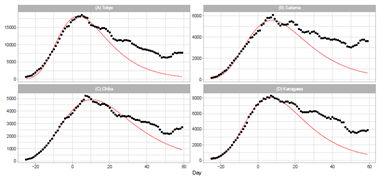
4.2.1 Tokyo Metropolitan Area: Ratings of population in Japan are Tokyo (1), Kanagawa (2), Saitama (5), and Chiba (6). The total population of these prefectures is approximately 29.3% of the Japanese population. A quasi-state of emergency began in these prefectures on January 21, 2022 (t = −10) as Japan tried to minimize the economic impact to specific areas where infections were again rising, and lifted this state on March 21,2022 (t = 49).

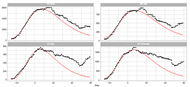
Figure 3: Gumbel model estimation of daily number of infections based on the data of pre- fectures in the Tokyo area: (A) Tokyo, (B) Saitama, (C) Chiba, and (D) Kanagawa. The results of the reported data are indicated by black points. The theoretical estimations are indicated by solid red lines. The vertical axis shows the daily counts, which were obtained using the parameters presented in Table 2.

Figure 3 demonstrates the daily number of infections for four prefectures in the Tokyo area. The theory provides a lower estimation than reported data for Tokyo, Saitama, and Kanagawa. In particular, the discrepancy is significant for Tokyo. As listed in Table 3, the ratio Rc of Tokyo is the second largest among 16 prefectures. In contrast, the calculated time-series data for Chiba approximately follow the trend of the reported data, and Pc for Chiba is very small compared with Pc for the three other prefectures.

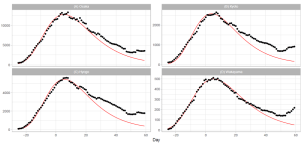
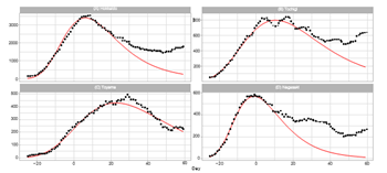
4.2.2 Osaka Metropolitan Area: Ratings of population in Japan are Osaka (3), Hyogo (7), Kyoto (13), and Wakayama (40). The total population of these prefectures is approximately 14.1% of the Japanese In Osaka, Kyoto, and Hyogo, a quasi-state of emergency began on January 27, 2022 (t = -4) and was lifted on March 21, 2022 (t = 49). In Wakayama, this measure began on February 5, 2022 (t = 5) and was lifted on March 6, 2022 (t = 34). Figure 4 shows the daily number of infections for four prefectures in the Osaka area. The plots for Osaka and Wakayama demonstrate reasonable fitting of the model to the reported data. Although the fitting qualities of Kyoto and Hyogo are not so good as Osaka and Wakayama, the Gumbel model can fit the data at a reasonable level. Table 3 illustrates the goodness-of-fit with small values of Pc for Osaka and Wakayama and with relatively larger values for Kyoto and Hyogo. Overall, the quality of fitting to the reported data for the Osaka region is better than that for the Tokyo region.

Figure 4: Gumbel model estimation of daily number of infections based on the data for prefectures in the Osaka metropolitan area: (A) Osaka, (B) Kyoto, (C) Hyogo, and (D) Wakayama. The results for the reported data are indicated by black points. The theoretical estimations are indicated by solid red lines. The vertical axis shows the daily counts, which were obtained using the parameters presented in Table 2.

4.2.3 Nagoya Metropolitan Area:

Ratings of population in Japan are Aichi (4), Shizuoka (10), Gifu (17), and Mie (22). The total population of these prefectures is approximately 11.8% of the Japanese A quasi-state of emergency began in Aichi and Gifu on January 21, 2022 (t = -10) and was lifted on March 21, 2022 (t = 49). In Mie, this measure began on January 21 (t = -10) and was lifted on March 6 (t = 34). In Shizuoka, this measure began on January 27 (t = -4) and was lifted on March 21 (t = 49). Figure 5 presents the results of the Gumbel model estimation for daily numbers for four prefectures in the Nagoya area. The Gumbel model can explain well the reported data for Aichi and Gifu. In contrast, the model gives poor results for Mie and Shizuoka. The Pc values for Aichi and Gifu are approximately the same as that for Osaka. Kanagawa is a neighboring prefecture of Shizuoka, and the Pc of both Kanagawa and Shizuoka prefectures are similar at 1.6 and 1.5.

4.2.4 Other Areas:

Ratings of population in Japan are Hokkaido (8), Tochigi (18), Nagasaki (27), and Toyama (37). The total population of these prefectures is approximately 7.5% of the Japanese A quasi-state of emergency began in Hokkaido and Tochigi on January 27, 2022 (t = -4) and was lifted on March 21, 2022 (t = 49). In Nagasaki, this measure began on January 21 (t = -10) and was lifted on March 6 (t = 34). Figure 6 reports the results of the analysis for prefectures in other areas. The model reproduces the data of Hokkaido in t ≤ 23 and then begins to underestimate the data in the decreasing phase. As shown in Fig.6 (B), the data for Tochigi shows a double-top shape, and we cannot use the window of [1, 12]. The estimate using the window of [-11, 0] well reproduces the reported data in t ≤ 35. For Toyama, the model well estimates almost all data points and has the smallest value of Pc. Although Nagasaki reports the largest value of Pc among 16 prefectures, the model can reproduces the data in t ≤ 10.

5. Discussion

The present method makes use of the Gumbel distribution as a model for the daily number of infections. In the model, there are three parameters: total

Figure 5: Gumbel model estimation of the daily number of infections based on the data for prefectures in the Nagoya area: (A) Aichi, (B) Gifu, (C) Mie, and (D) Shizuoka. The results of reported data are indicated by black points. The theoretical estimations are indicated by solid red lines. The vertical axis shows the daily counts, which are obtained using parameters presented in Table 2.

Figure 6: Gumbel model estimation of the daily number of infections based on the data for prefectures in other areas: (A) Hokkaido, (B) Tochigi, (C) Toyama, and (D) Nagasaki. The results for the reported data are indicated by black points. The theoretical estimations are indicated by solid red lines. The vertical axis shows the daily counts, which are obtained using the parameters presented in Table 2.

Figure 7: Probability density functions for Kyoto and Hyogo. The probability density for Kyoto is indicated by blue points, and that for Hyogo is indicated by red points. The vertical axis shows the probability. Day 1 is January 30 for Kyoto and February 1 for Hyogo.

Number N_e, shape parameter a, and position parameter b. For the estimation of the parameters, the present study applies two-step transformations to the sum of daily numbers U_t. The first step involves taking the ratio M_t of the seven-day moving average m_t to U_t as given in Eq. (4). By this step, the parameter N_e is eliminated from the equation. The second step is the logarithmic transformation L_t given by Eq. (6). Then, parameters a and b can be estimated by regression analysis.

The present research is inspired by the analysis of COVID-19 data by Nakano and Ikeda [21]. Nakano and Ikeda introduced a new indicator K_t as a measure of spread rate

Note that K_t does not have the parameter of total number. It is easy to show that K_t can be rewritten as

Which has similar form as M_t.

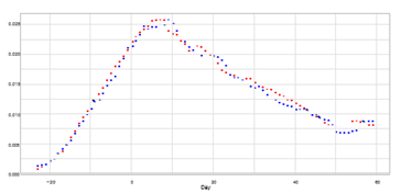
Table 2 reports that the shape parameters of Kyoto and Hyogo take almost equal values, and Fig. 4 shows the close resemblance of plots for both prefectures. Figure 7 shows the probability density functions for Kyoto and Hyogo. The estimation of the probability function is obtained by dividing the seven-day moving average m_t by the estimated total number Ne. Since the difference of position parameter b is 5:078 − 3:462 ≈ 2, we shift the data for Kyoto to a position two days later. The result meets our expectation, and the probability density functions for both prefectures match well. Kyoto and Hyogo are neighbouring prefectures, and a large amount of traffic volume is supported by railroads and highways spread throughout the Osaka area. However, the result may not be explained by this observation alone and requires more detailed analysis.

6. Conclusion

A mathematical model that captures the characteristic of infections is a key tool to support science-based decision-making and to provide a quantitative assessment of exit strategies. In the present study, we apply the Gumbel distribution function of the EVT for the analysis of time-series data of the sixth-wave COVID-19 outbreak in Japan. Selecting 16 prefectures out of the 47 prefectures in Japan, we estimate the growth rate of infection and the point of inflection for each prefecture. For seven prefectures, the daily numbers of infections are well described by the Gumbel distribution model. The value of Pc in Table 3 is less than 1.3 for Chiba, Osaka, Wakayama, Aichi, Gifu, Tochigi, and Toyama. This table also indicates lack-of-fit for several prefectures. The value of Pc is greater than 1.5 for Tokyo, Saitama, Kanagawa, Mie, Shizuoka, and Nagasaki. Thus, this fact suggests that more detailed modeling would be required. The present model assumes that future data can be estimated by extrapolation of a linear function. However, Fig. 1 indicates that the reported data for infection deviate significantly from the linear trend. We are now trying to develop a method to overcome this problem.

Author Contributions

The present study was conducted equally by the authors.

Competing Interests

The authors declare no competing interests.

References

1. Kermack WO, McKendrick AG. A contribution to the mathematical theory of epidemics. Proc. Roy. Soc. London A 115(1927): 700-721.
2. Li MY. An Introduction to Mathematical Modeling of Infectious Diseases. Springer (2018).
3. Brauer F. Compartmental models in epidemiology. In: Mathemat- ical Epidemiology. Lecture Notes in Mathematics 1945 (2008): 19-79.
4. Zou Y, Pan S, Zhao P, et al. Outbreak analysis with a logistic growth model shows COVID-19 suppression dynamics in China, PLoS ONE 15 (2020): e0235247.
5. Wieland T. A phenomenological approach to assessing the e?ectiveness of COVID-19 related nonpharmaceutical interventions in Germany. Saf. Sci 131 (2020): 104924.
6. Keeling MJ, Hill EM, Gorsich EE, et al. Predictions of COVID-19 dynamics in the UK: Short-term forecasting and analysis of potential exit strategies. PLoS. Comput. Biol 17 (2021): e1008619.
7. Chowell G, Sattenspiel L, Bansal S et al. Mathematical models to characterize early epidemic growth: A review. Phys. Life Rev 18 (2016): 66-97.
8. Chen J, Lei X, Zhang L, et al. Using extreme value theory approaches to forecast the probability of outbreak of highly pathogenic influenza in Zhejiang, China. PLoS ONE 10 (2015): e0118521.
9. Wong F, Collins JJ. Evidence that coronavirus superspread- ing is fat-tailed. PNAS 117 (2020): 29416-29418.
10. Gumbel J. Statistics of Extremes, Columbia University Press. New York (1958).
11. Coles S. An Introduction to Statistical Modeling of Extreme Values. Springer-Verlag, London (2001).
12. Asadi ZS, Melchers RE. Extreme value statistics for pitting corrosion of old underground cast iron pipes, Reli. Engneer. Sys. Safe 162 (2017): 64-71.
13. Medford A. Best-practice life expectancy: An extreme value approach. Demo. Res 36 (2017): 989-1014.
14. Fisher RA, Tippett LHC. Limiting forms of the fre- quency distribution of the largest or smallest members of a sample. Proc. Cambridge Philos. Soc 24 (1928): 180-190.
15. Ohnishi A, Namekawa Y, Fukui T. Universality in COVID- 19 spread in view of the Gompertz function. Prog. Theor. Exp. Phys (2020): 123J01.
16. Furutani H, Hiroyasu T, Okuhara Y. Method for estimating time series data of COVID-19 deaths using a Gumbel method, Arch. Clin. Biomed. Res 6 (2022): 50-64.
17. Carter JT, Challenor PG. Methods of fitting the Fisher- Tippett type 1 extreme value distribution. Ocean Engng. 10 (1983): 191-199.
18. Hwang HK, Panholzer A, Rolin N, et al. Probalistic analysis of the (1+1)-evolutionary algorithm. Evol. Comput 26 (2018): 299-345.
19. Ikeda S, Zhang Y, Furutani H, et al. Runtime analysis of linear functions using Markov chain method. Proc (2021): 4pages.
20. Zhang Y, Qin X, Ma Q, et al., Markov chain analysis of evolu- tionary algorithms on OneMax function: From coupon collector’s problem to (1+1) EA. Theo. Com. Sci 820 (2020): 26-44.
21. Nakano T, Ikeda Y. Novel indicator to ascertain the status and trend of COVID-19 spread: Modeling study. J. Med. Internet Res 22 (2020): e20144.