Analysis and Evaluation of Non-Pharmaceutical Interventions on Prevention and Control of COVID-19: A Case Study of Wuhan City

Abstract

As the threat of COVID-19 increases, many countries have carried out various non-pharmaceutical interventions. Although many studies have evaluated the impact of these interventions, there is a lack of mapping between model parameters and actual geographic areas. In this study, a non-pharmaceutical intervention model of COVID-19 based on a discrete grid is proposed from the perspective of geography. This model can provide more direct and effective information for the formulation of prevention and control policies. First, a multi-level grid was introduced to divide the geographical space, and the properties of the grid boundary were used to describe the quarantine status and intensity in these different spaces; this was also combined with the model of hospital isolation and self-protection. Then, a process for the spatiotemporal evolution of the early COVID-19 spread is proposed that integrated the characteristics of residents’ daily activities. Finally, the effect of the interventions was quantitatively analyzed by the dynamic transmission model of COVID-19. The results showed that quarantining is the most effective intervention, especially for infectious diseases with a high infectivity. The introduction of a quarantine could effectively reduce the number of infected humans, advance the peak of the maximum infected number of people, and shorten the duration of the pandemic. However, quarantines only function properly when employed at sufficient intensity; hospital isolation and self-protection measures can effectively slow the spread of COVID-19, thus providing more time for the relevant departments to prepare, but an outbreak will occur again when the hospital reaches full capacity. Moreover, medical resources should be concentrated in places where there is the most urgent need under a strict quarantine measure.

1. Introduction

In December 2019, the coronavirus disease 2019 (COVID-19) spread across the world. Due to its characteristics of a high infection rate, incubation period, and asymptomatic infection, the virus quickly spread among the population, coming as an unprecedented blow to human life, economic development, and social stability [1,2,3,4]. In the absence of an effective vaccine, countries had to implement effective interventions as soon as possible to alleviate the spread of COVID-19, such as strict quarantine measures, wearing facemasks, school closures, and large-scale testing [5]. However, the unknown and sudden nature of the virus made it difficult for countries to implement scientific and reasonable emergency policies as early as possible. Meanwhile, the large-scale personnel deployment and resource distribution, as well as the implementation of the policy plan, also require a long period of preparation. Therefore, the implementation scope, implementation scale, intervention time, and potential effect of prevention and control measures are key factors that need to be decided upon urgently for all countries suffering from different degrees of the spread of COVID-19. Making these decisions quickly will provide important support for the implementation of scientific and effective prevention and control measures.

Early studies carried out on COVID-19 mainly focused on epidemiology, which can be roughly divided into three aspects: the estimation of the epidemiology parameters, the forecasting of the epidemic situation, and the analysis of the effectiveness of intervention measures. In the early stages of the outbreak of COVID-19, the basic reproduction number, incubation period, and other epidemic parameters were estimated using the early reported case data and overseas export data, which was helpful for understanding the dynamic transmission mechanism of COVID-19 while preliminarily assessing the epidemic risk level [6,7,8,9,10]. Subsequently, the future epidemic situation was predicted by fitting the reported case data based on improved compartmental models. For example, the susceptible, exposed, infected, quarantined, recovered (SEIQR); the susceptible, infected, removed-X (SIR-X); and the susceptible, infectious, quarantined, recovered (SIQR) models were proposed [11,12,13]; a zonal susceptible, exposed, infected, recovered, deceased (SEIRD) model combining the spatial diffusion and heterogeneity of infectious diseases was proposed [14]; and the susceptible, exposed, infectious, recovered, susceptible (SEIRS) model with an exponential structure was proposed [15]. Similarly, new dynamic transmission models of infectious disease were developed by adding asymptomatic infectors and environmental infection to the susceptible, exposed, infectious, recovered (SEIR) model [16,17,18,19,20]. Some stochastic-based regression models were used to forecast the phenomena in as many as ten of the most affected states of Brazil [21]. A hybrid ARIMA-WBF model was considered for forecasting different COVID-19-infected countries worldwide [22] and a three-stage exposed, infected, susceptible, hospital, recovered (e-ISHR) model introducing the time delay mechanism was established [23]. A discrete multi-stage dynamics system with time delay based on the development process of China’s epidemic was established [24], while the evolution of the epidemic spread was simulated by introducing the statistical characteristics of complex network distribution into an epidemiological model [25,26]. However, most of these models focus on the time series analysis of the spread of COVID-19. Such model parameters have a clear epidemiological significance but lack a spatiotemporal description of practical significance. With the positive effects gained by epidemic prevention and control in some countries, the effect of implementing different epidemic prevention and control measures on the alleviation of the epidemic situation has been evaluated, such as quarantines [6,13,18,27,28,29], wearing face masks [16,30], social distancing [16,18,30,31], travel restrictions [32,33], the tracking and isolation of cases [16,34], school closures [18], the protection of the elderly over 70 years old [18], hospital isolation [23,35] and external factors (ventilation and hand washing) [36,37,38,39]. The effect of these interventions has been evaluated by performing statistical analyses of the trend of the epidemic data of some countries that implemented different interventions [40,41,42]. However, the main aim is to estimate the effectiveness of intervention measures by adjusting the mathematical parameters of the model to simulate the trend of the epidemic when different intervention measures are used based on the prediction model. However, there is no reasonable explanation for the mapping between the model parameter values and the practical significance of the application of special interventions—for example, what scale of the isolation measures is needed that would be equivalent to a 30% reduction in contact rate? At the same time, these studies seldom consider that the spatiotemporal evolution of COVID-19 may have different impacts on epidemic interventions. Moreover, most of these models are mainly based on the compartmental model and take the epidemic area as a whole; thus, they lack detailed spatial information. Therefore, it is difficult to obtain information about the spatial spread of COVID-19. Therefore, the question of how to use the quantitative method to integrate spatial information and the impact of interventions into the traditional classical compartmental model based on a time series process is the focus of our scientific research.

Geography is a subject that researches the spatial distribution rule, spatiotemporal evolution process, and regional features of the geographical elements and has been widely applied in various fields. The process of the spread and infection of COVID-19 is influenced by a series of complex natural and social factors. Its mode of transmission must usually be through close contact. Therefore, its most important feature is the process of spatiotemporal spread—that is, its transmission is regular in terms of time series and geospatial elements, which leads to understanding a phenomenon as geographical and potentially mappable [43,44]. Recently, there are many studies conducted in this field. For example, the mobile phone location data were used to forecast the epidemic situation in Wuhan from the perspective of spatial interaction [45]. The association between American nursing home-level metrics and place-based variables with COVID-19 confirmed that cases in nursing homes across the United States were established using spatial modeling technology [46]. The ecological niche model (ENM) was utilized to assemble the epidemic data and nine socioeconomic variables to identify the potential risk zones in Beijing, Shenzhen, and Guangdong [47]. However, the detailed observation data of crowds, such as the spatial interaction data of crowds and resident activity data, are difficult to obtain in a public health and safety emergency, usually resulting in the problem of missing or incomplete coverage. Although these studies have used multi-source data to analyze the epidemic situation, they still belonged to the categories of observation and reasoning with a small amount of sample data because of the precision and resolution of the data. Moreover, most of the current epidemic-related data only include the location where patients first showed symptoms, leaving the location where the patients were infected unknown. This indicates that current epidemic-related data also have a backtracking problem. Thus, the question of how to build observation strategies and scientific methods that are in line with reality is the key problem in the current public health and safety emergency [48].

In this paper, we propose a COVID-19 prevention and control model based on a discrete grid. The goals of this study are two-fold: first, to evaluate and quantify the impacts of interventions by integrating a time series dynamic model of COVID-19 and spatial information; second, to establish a connection between the model parameters and the practical application significance, and not simply adjusting the mathematical parameters of the model to illustrate the effectiveness of the interventions. Our model parameters were the scope of the actual area and the intensity of the measures, which can provide better and more direct information for public health and safety emergencies policy [49]. Therefore, a multi-level grid was used to divide the geographical space of the epidemic area, and the status and intensity of the quarantine of the sub-region were described by dotted and solid lines of the boundary and the size of the grid, respectively. Then, a hospital isolation model was constructed by allocating medical capacity to the affected sub-region according to the correlation between the spatial distribution of hospitals and the sub-region. In addition, the parameters of means for human self-protection human (including wearing a face mask, washing hands frequently, and ventilation) were introduced into the dynamics model of COVID-19 to achieve the modeling of self-protection measures. In the absence of detailed behavior tracking data, we assumed that the means of transmission of COVID-19 mainly started from the space adjacent to the infected path and then gradually spread to the surrounding region (without any interventions) [50]. The spatiotemporal spread evolution of COVID-19 was simulated through the behavior features of residents’ daily activities based on the spatial correlation between sub-regions. Then, the COVID-19 dynamics model with asymptomatic infection was introduced for analyzing and quantifying the infectious situation of COVID-19 under the effects of different interventions. Since the absence of early epidemic data for Wuhan was caused by early interventions and the unknown nature of the virus, while the epidemic prevention and control measures abroad were applied relatively late and were lax [19], the early reported case data of the U.K., the U.S., Spain, and Germany were used to discuss the status of the spread of COVID-19. The parameters of a dynamic model of COVID-19 free spread were brought to Wuhan to obtain the infected curve of Wuhan without any interventions. Then, the potential of quarantine measures, hospital isolation measures, and self-protection measures to alleviate the spread of the epidemic at different scales and with different intervention times were discussed. Finally, the rationality and correctness of the model were evaluated with the actual data of Wuhan, including epidemic data, hospital distribution data, and medical attribute data. The novelties of this study are highlighted as follows:

(I). The association between the model parameters and the geographical space is established from the perspective of geography. This provides the model parameters practical instructive significance for special interventions rather than them only being used to describe the effect of the prevention and control measures, which can provide more direct and effective information for the formulation of prevention and control policies;

(II). The effect of hospital isolation measures is evaluated by calculating the number of patients admitted to hospitals in the each infected region from the perspective of the hospital spatiotemporal distribution.

2. Materials and Methods

2.1. Data

Wuhan reported a “viral pneumonia of unknown origin” on 31 December 2019, then issued a “city-wide closure”. The government successively issued a series of measures, such as restricting transportation, closing school, closing entertainment places, and prohibiting public gatherings. At the same time, many designated hospitals such as “huoshenshan” and “leishenshan”, as well as “fangcang” shelter hospitals, began to be put into use. Medical staff and medical resources from all over the country were involved in the fight against COVID-19. In order to discuss the effect of different interventions to alleviate the spread of COVID-19, this study collected global epidemic data, including the number of confirmed cases per day and the cumulative number of cured people and deaths from dingxiangyuan (https://ncov.dxy.cn/ncovh5/view/pneumonia; 1 June 2020) and the COVID-19 Data Repository by the Center for Systems Science and Engineering (CSSE) at Johns Hopkins University [51]; the data of designated hospitals in Wuhan, including the spatial distribution of hospitals, the intervention time, the number of open beds and the cumulative number of patients from Wuhan Municipal Health Commission (http://zwfw.hubei.gov.cn/webview/yqzq/index.html; 20 June 2020); and the data of the medical resources gathered in Wuhan, including the number of local registered medical staff, the number of supporting medical staff in different regions, and the number of face masks (including N95 masks and medical–surgical masks) from the websites of the Hubei Provincial Bureau of Statistics, Hubei Provincial People’s Government (http://tjj.hubei.gov.cn/ztzl/jjdyqqfkjjz/zxtb/; 20 June 2020), and People’s Daily (http://www.people.com.cn/; 20 June 2020). The authors organized and stored the data in the zenodo public database; the corresponding data links are listed at the end of this article.

From the daily number of reported new cases in Wuhan, it can be seen that a sudden surge occurred on 12 February 2020 (

Table 1. Calibration data of the cases reported per day in Wuhan.

Date	Actual Value	Calibration Data
30 January 2020	378	759
31 January 2020	576	1101
1 February 2020	894	1182
2 February 2020	1033	1574
3 February 2020	1242	1683
4 February 2020	1967	2082
5 February 2020	1766	2195
6 February 2020	1501	2542
7 February 2020	1985	2618
8 February 2020	1378	2856
9 February 2020	1921	2857
10 February 2020	1552	2949
11 February 2020	1104	2852
12 February 2020	13436	3212

). The reason for this is that the Novel Coronavirus (2019-nCoV) Nucleic Acid Detection Kit (PCR fluorescence probing) was changed to clinical diagnosis (including the computed tomography (CT) method). Although, it was unjustified for later verification. This problem was analyzed through Richards nonlinear curve model [52], and, according to the incubation period of COVID-19 lasting for 7~14 days, the calibrated daily number of new confirmed cases from 30 January 2020, to 12 February 2020, is shown in Table 1.

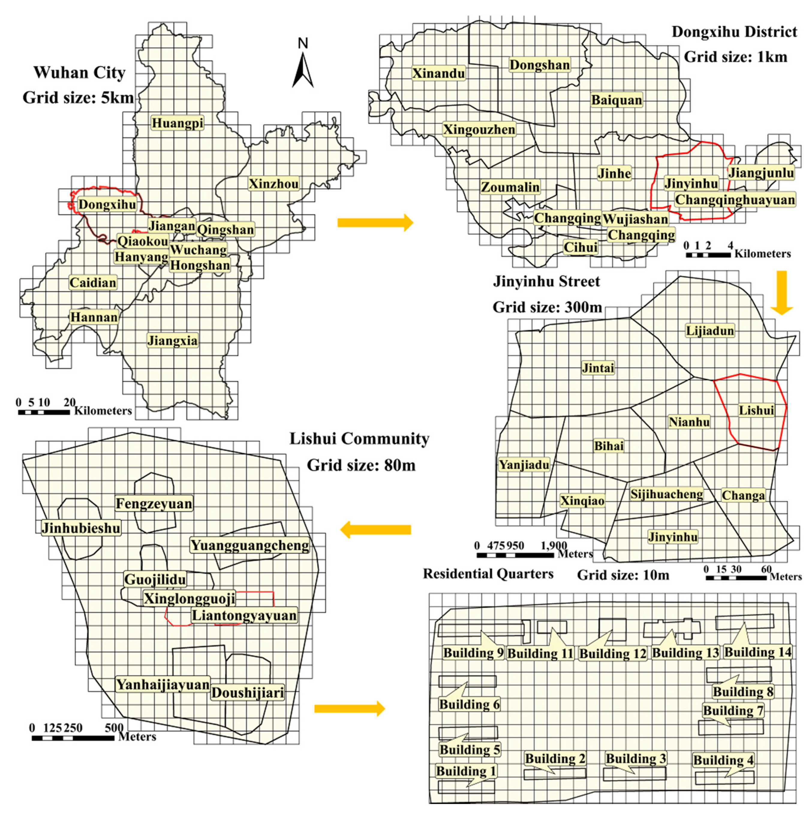
2.2. Medel of Quarantine Measures Based on a Discrete Grid

Quarantine measures usually take the “province–city–district–street–community–village–home” as the basic unit to limit the scope of people’s activity, which greatly reduces the contact between infected people and susceptible individuals. However, the uncertainty of the size and irregular shape of this traditional unit of prevention and control can cause great difficulties in the modeling. Moreover, more precise administrative division data are usually not easy for other authors to obtain. As shown in Figure 1, the prevention and control units of “city–district–street–community–home” can use different levels of the grid to make up for the difficulty of data acquisition and the irregular shape, and the effective grid regions were limited within the effective areas within the administrative division. According to the spatial features of physical quarantine, the discretization of the geospatial area was realized by a multi-level discrete grid with different sizes and series of grid units. An adaptive statistical unit can be formed by a hierarchical geographic grid to fill the traditional prevention and control unit. At the same time, the dotted and solid lines of the boundary and size of the grid can be used to describe the status and intensity of the quarantine in different regions, respectively, and the distribution of the grid can map the practical scope of the implementation of quarantine measures.

The specific design was as follows: The research areas were divided into different sub-regions using a discrete grid, in which the total number of sub-regions was denoted by n. Referring to the model of COVID-19 spread dynamics proposed by Okuonghae et al. [16], the total number of humans in the epidemic area, denoted by N, was split into susceptible humans S(t), exposed humans E(t), asymptomatic infectious humans A(t), symptomatic infectious humans I(t), infected humans detected via testing C(t), and recovered humans R(t). The boundary of the grid was represented with a dotted line before the implementation of quarantine (Figure 2). At this time, there were few restrictions on the contact between people, and the spread of COVID-19 occurred freely. The numerical changes of each human could be quantified by the epidemic dynamic model of the whole region, as shown in the following Equations (1)–(6). The related variable parameters of the model are described in

Table 2. Description of the parameters of the COVID-19 spread dynamics model.

Parameter	Interpretation
$S_i^t$	Number of susceptible humans per day in grid cell i.
$E_i^t$	Number of exposed humans per day in grid cell i (infected but not infectious).
$A_i^t$	Number of asymptomatically infectious humans per day in grid cell i (undetected).
$I_i^t$	Number of symptomatically infectious humans per day in grid cell i (undetected).
$C_i^t$	Number of infectious humans detected per day in grid cell i (including asymptomatic and symptomatic, tested but not completely admitted to hospital).
$R_i^t$	Number of recovered humans per day in grid cell i.
${\beta }_0$	Effective spread rate.
$\sigma$	Progression rate from exposed state to the infectious state.
$\upsilon$	Fraction of new infectious humans that are asymptomatic.
$\alpha$	Modification parameter that accounts for the reduced infectiousness of humans in the A class when compared to humans in the I class.
${\gamma }_a,{\gamma }_o,{\gamma }_c$	Recovery rate for individuals in the A, I, and C classes, respectively.
$\phi$	Detection rate (via contact tracing and testing) for the I class.
$\theta$	Detection rate (via contact tracing and testing) for the A class.
$d_o,d_c$	Disease-induced death rates for individuals in the I and C classes, respectively.

.

$$S_t=S_1-{\displaystyle {\displaystyle \sum }_{j=1}^{t-1}\left(\frac{{\beta }_0\left(\alpha A_j+I_j\right)}{N-C_j}{S}_j\right)},$$

(1)

$$E_t=E_1+{\displaystyle {\displaystyle \sum }_{j=1}^{t-1}\left(\frac{{\beta }_0\left(\alpha A_j+I_j\right)}{N-C_j}{S}_j-\sigma E_j\right)},$$

(2)

$$A_t=A_1+{\displaystyle {\displaystyle \sum }_{j=1}^{t-1}\left(\upsilon \sigma E_j-\left(\theta +{\gamma }_a\right)A_j\right)},$$

(3)

$$I_t=I_1+{\displaystyle {\displaystyle \sum }_{j=1}^{t-1}\left(\left(1-\nu \right)\sigma E_j-\left(\phi +{\gamma }_o+d_o\right)I_j\right)},,$$

(4)

$$C_t=C_1+{\displaystyle {\displaystyle \sum }_{j=1}^{t-1}\left(\theta A_j+\phi I_j-\left({\gamma }_c+d_c\right)C_j\right)},$$

(5)

$$R_t=R_1+{\displaystyle {\displaystyle \sum }_{j=1}^{t-1}\left({\gamma }_c{C}_j+{\gamma }_a{A}_j+{\gamma }_o{I}_j\right)}.$$

(6)

When quarantine measures were implemented, all of the grid boundaries changed from dotted to solid lines, and the current time was denoted t₀. The activities of people were limited to within the sub-regions, meaning that COVID-19 could only diffuse in the infected grid regions and could not affect the other grid regions (Figure 2). The number of different humans in the sub-grid was denoted by $S_i^t$, $E_i^t$, $A_i^t$, $I_i^t$, $C_i^t$ and $R_i^t$ at time t, respectively. The numerical changes of each human were the sum of all sub-regions, as shown in the following Equations (7)–(12), where $N_i$ refers to the number of people in each grid cell, and its specific value was obtained from the statistical yearbook data using Kriging interpolation [50]:

$$S_t={\displaystyle {\displaystyle \sum }_{i=1}^n\left(S_i^{t_0}-{\displaystyle {\displaystyle \sum }_{j=1}^{t-1}\frac{{\beta }_0\left(\alpha A_i^j+I_i^j\right)}{N_i-C_i^j}{S}_i^j}\right)},$$

(7)

$$E_t={\displaystyle {\displaystyle \sum }_{i=1}^n\left(E_i^{t_0}+{\displaystyle {\displaystyle \sum }_{j=1}^{t-1}\left(\frac{{\beta }_0\left(\alpha A_i^j+I_i^j\right)}{N-C_i^j}{S}_i^j-\sigma E_i^j\right)}\right)},$$

(8)

$$A_t={\displaystyle {\displaystyle \sum }_{i=1}^n\left(A_i^{t_0}+{\displaystyle {\displaystyle \sum }_{j=1}^{t-1}\left(\upsilon \sigma E_i^j-\left(\theta +{\gamma }_a\right)A_i^j\right)}\right)},$$

(9)

$$I_t={\displaystyle {\displaystyle \sum }_{i=1}^n\left(I_i^{t_0}+{\displaystyle {\displaystyle \sum }_{j=1}^{t-1}\left(\left(1-\nu \right)\sigma E_i^j-\left(\phi +{\gamma }_o+d_o\right)I_i^j\right)}\right)},$$

(10)

$$C_t={\displaystyle {\displaystyle \sum }_{i=1}^n\left(C_i^{t_0}+{\displaystyle {\displaystyle \sum }_{j=1}^{t-1}\left(\theta A_i^j+\phi I_i^j-\left({\gamma }_c+d_c\right)C_i^j\right)}\right)},$$

(11)

$$R_t={\displaystyle {\displaystyle \sum }_{i=1}^n\left(R_i^{t_0}+{\displaystyle {\displaystyle \sum }_{j=1}^{t-1}{\gamma }_c{C}_j+{\gamma }_a{A}_j+{\gamma }_o{I}_j}\right)}.$$

(12)

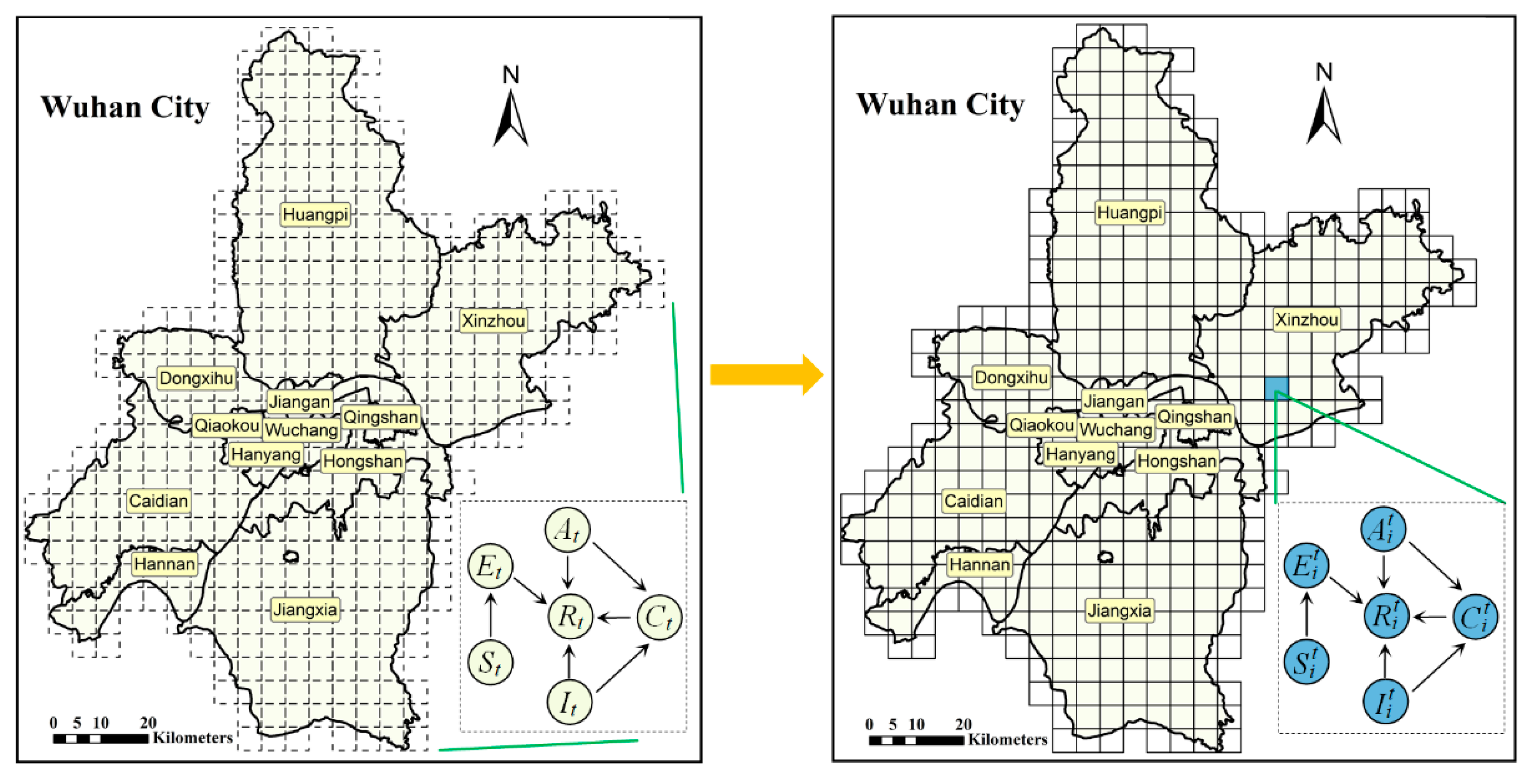
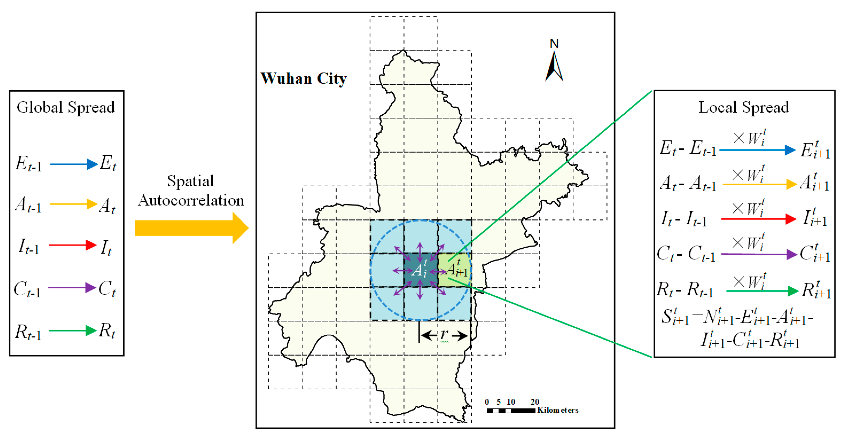
2.3. Spatiotemporal Spread Model of COVID-19 Based on a Discrete Grid

The most important feature of infectious diseases is that, in order for them to spread, they need a special path of spread, such as air spread, droplet spread, close contact, and blood spread. Government departments usually take interventions to cut off the transmission path between infected and susceptible humans, such as implementing strict quarantine measures, testing, tracking cases, wearing face masks, and actively keeping a distance from patients with a fever. Therefore, it is necessary to determine the distribution of the number of infected humans in each grid region before a quarantine is implemented in order to evaluate the effect of different interventions.

The differences in regions and virus types mean that the spatiotemporal spread mode, spread path, and spread capacity of infectious diseases have certain differences. However, because of the spatial correlation of people’s living, work, range of activities, and surrounding environment, the transmission of infectious diseases restricted by those spatial factors also has spatial correlations. When the flow of people in an epidemic area is not completely limited, the number of newly infected people in a sub-region at a certain time is not only affected by the number of infected people at the previous time, but also by the number of infected people in the surrounding regions. The transmission of infectious diseases similar to COVID-19 usually starts from the space adjacent to the infected path of the virus and then gradually spreads to the surrounding regions [50]. As shown in Figure 3, the patients in the infected area $A_i^t$ are most likely to infect the people in the eight nearby areas (light blue area) next. Therefore, the epidemic area was intersected with a buffer of infected grid cells constructed by the behavior features of people’s average activities to obtain the number of newly infected grid regions each day, where the radius is denoted by r. An incompletely infected grid cell was regarded as infected for the convenience of calculation. In order to ensure the consistency of the diffusion scale, we used the maximum grid scale of the experiment (1000 m) as the basis for diffusion.

In the process of the transmission of COVID-19, the number of cases of newly infected people per day always has a time series change process that first increases and then decreases. Meanwhile, infected people are abstracted as many discrete points in geographical space. According to Tobler’s first law of geography, the process of the transmission of COVID-19, as restricted by geographical spatial factors, has strong spatial correlation characteristics [44]. The distance is used to describe the spatial weight concept of the infected grid cells, which could help to obtain the number of newly infected people at the next moment in the corresponding infected grid cell, as shown in Figure 3 and Equations (13) and (14). In addition, the number of people should be rounded in the distribution:

$$W_i^t={\left(h_{ij}^t\right)}^{-p}/{\displaystyle {\displaystyle \sum }_{i=1}^{n^{{}_t}}{\left(h_{ij}^t\right)}^{-p}},$$

(13)

$$h_{ij}^t=\sqrt{{\left(x_i^t-x_j^{t-1}\right)}^2+{\left(y_i^t-y_j^{t-1}\right)}^2},$$

(14)

where $W_i^t$ is the weight of the number of newly infected crowds assigned by the infected grid cell, $h_{ij}^t$ is the distance from the infectious grid cell to the affected grid cell, $(x_i^{t-1},y_i^{t-1})$ is the coordinates of the center point of the infectious grid cell, $(x_j^{t-1},y_j^{t-1})$ is the coordinates of the center point of the affected grid cell, n^t is the number of affected grid cells, and $p$ is any positive real number (usually 2).

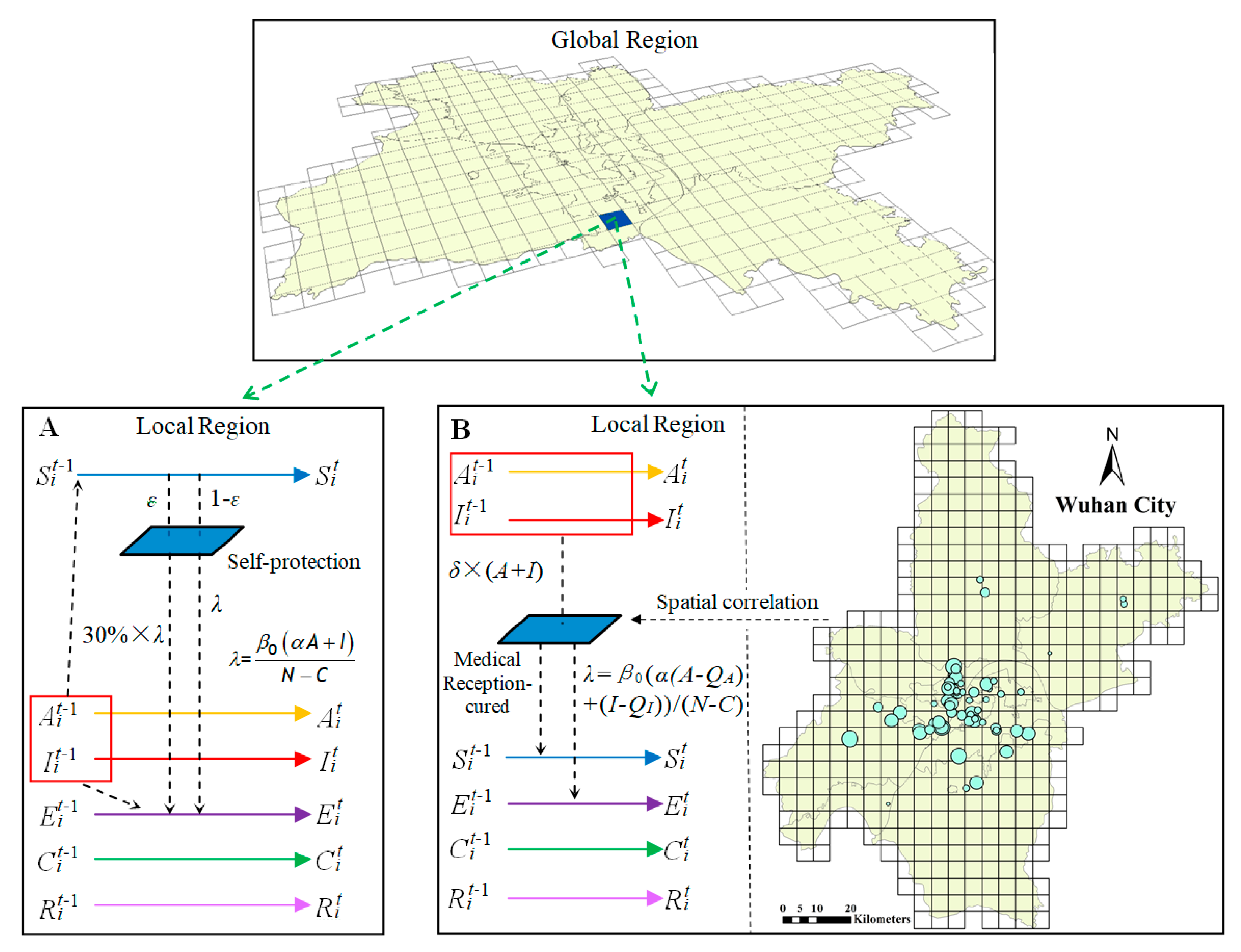
2.4. Model of Self-Protection Measures

During the outbreak of COVID-19, people took many self-protection measures, such as wearing face masks effectively, washing their hands frequently, keeping their houses ventilated, and maintaining distance from patients with a fever. Clinical and infectious disease studies have shown that the implementation of proper self-protection measures can effectively reduce the risk of infection and the external spread of the virus by 70–80% [53]. In this study, the parameter $\epsilon$ was introduced to represent the proportion of people who undertake effective self-protection measures. The probability of the infection of susceptible humans undertaking effective self-protection measures was reduced to 30% of the normal value. In contrast, the rate of infection and external spread to other humans remained unchanged (Figure 4A).

2.5. Model of Hospital Isolation Measures

During the spread of COVID-19, the government designated certain hospitals and outpatient clinics to detect and receive suspected COVID-19 patients. People typically go to a nearby hospital for diagnosis when they find themselves unhealthy, due to the influence of people’s living, work, activity range, and the surrounding environment. Therefore, the spatial distribution of hospitals and the number of beds available have a great impact on the spread of COVID-19. There is a strong spatial correlation between a geographical space and a hospital. If a patient is admitted to the hospital, they will no longer participate in the chain of transmission of infectious diseases. Considering the open time lag of medical beds and that government investment in medical beds is usually based on the number of people who are currently infected, the percentage parameter $\delta$ for the number of infected people was introduced to simulate the number of beds used in the hospital every day. Then, the number of cases admitted to the hospital every day was allocated to the corresponding infected grid cell based on the spatial distance weight (Figure 4B), where $Q_A$ and $Q_I$ refer to the number of asymptomatic and symptomatic infected people admitted to the hospital every day, respectively, and the specific values were mathematical products of ${\displaystyle {{\displaystyle \sum }}_{i=1}^n{Q}_i^t}$ and the corresponding detection ratio ($\theta$ and $\phi$). The number of daily patients put into hospital isolation in each grid cell is shown in the following Equations (15)–(17):

$${\mathrm{h}}_{ij}=\sqrt{{\left(x_i-x_j\right)}^2+{\left(y_i-y_j\right)}^2},$$

(15)

$$W_{ij}={\mathrm{h}}_{ij}{}^{-p}/{\displaystyle {\displaystyle \sum }_{j=1}^{n_i}{\mathrm{h}}_{ij}{}^{-p}},$$

(16)

$$Q_i^t=\{\begin{array}{l}0,t\le t_j^0\cup t\ge t_j^1\\ {\displaystyle {\displaystyle \sum }_{j=1}^H{w}_{ij}\times \delta \times \left(A_t+I_t\right)},t_j^0\le t\le t_j^1\end{array},$$

(17)

where $Q_i^t$ is the number of patients admitted to the hospital in the grid cell (including asymptomatic and symptomatic), $h_{ij}$ is the distance between the grid cell and the hospital, $w_{ij}$ is the assigned weight of the number of hospital patients in the corresponding grid cell, $(x_i,y_i)$ is the coordinates of the central point of the infected grid cell, $(x_j,y_j)$ is the coordinates of the hospital, $n_i$ is the number of grid cells affected by the hospital, and $t_j^0$ and $t_j^1$ are the intervention time and closing time of the hospital, respectively.

3. Results

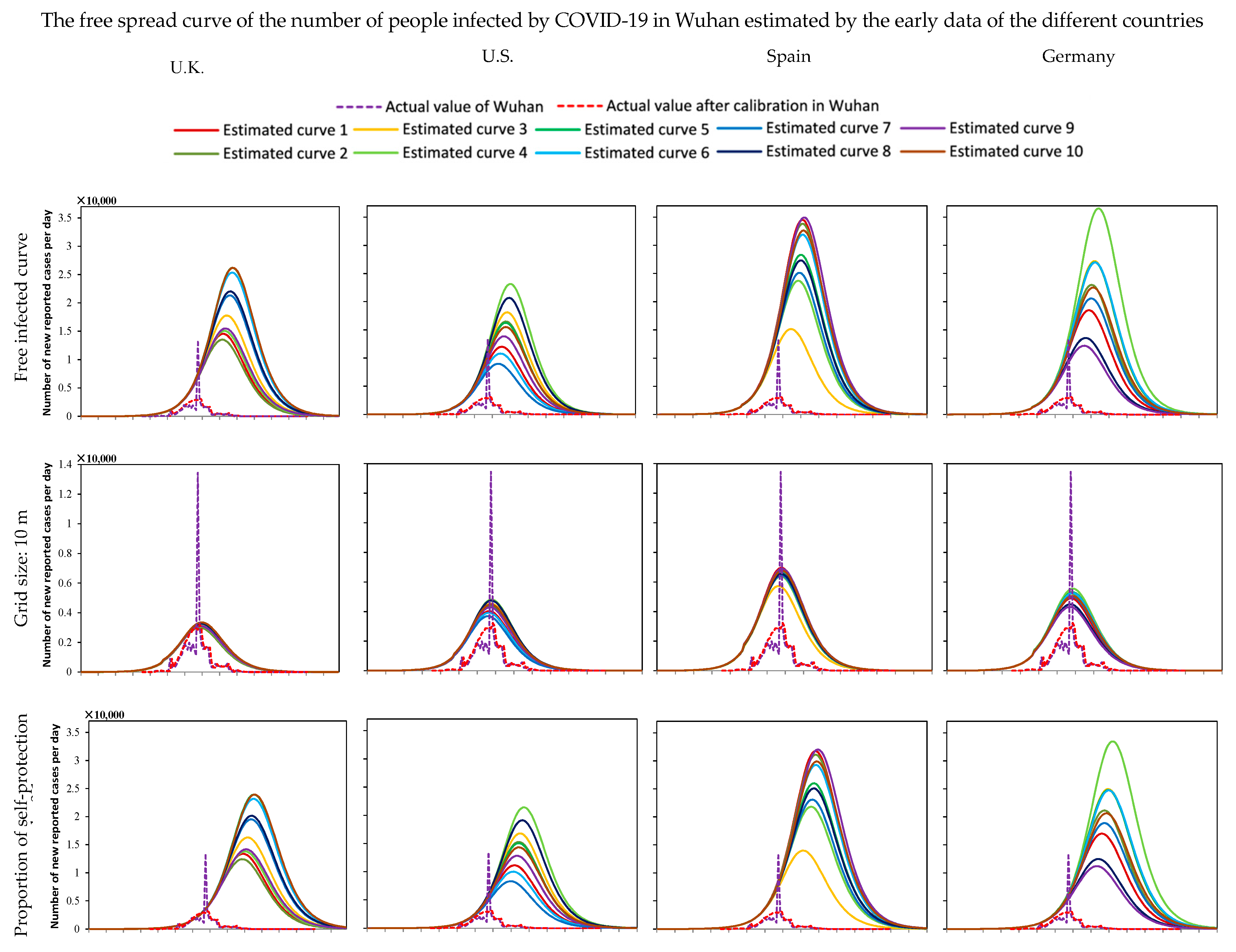
3.1. Numerical Simulation and Analysis of the Number of Infected Humans without Any Interventions

In order to compare the differences in the number of infected humans before and after the interventions, the curve of people infected without any intervention needed to be estimated. The first thing that needs to be made clear is that no country will allow infectious diseases to spread freely, which means that the freely infected curve representing the number of infected humans for any infectious diseases is usually not available. Recently, many studies have used the early epidemic data of the study area or random sampling of the basic reproduction number R₀ to solve this problem [16,18]. Unfortunately, Wuhan was the first city that faced the COVID-19 epidemic. Due to the unknown characteristics of the virus and the rapid and intensive interventions carried out, the estimated number of infected humans detected at this early stage is very unreliable. Therefore, it cannot truly describe the early trend of the number of infected humans. However, as foreign epidemics occurred after the outbreak in Wuhan, the level of medical detection was high and interventions carried out in foreign regions were relatively late and lax [19]; it is more likely that these early epidemic data are consistent with the free spreading situation of COVID-19. However, the differences between different countries in terms of the patterns of movement of crowds and levels of economic development make it difficult to objectively clarify which country’s data are the most appropriate for simulating the free infected trend of COVID-19. Therefore, for this study, we selected early epidemic data from the U.K., the U.S., Spain, and Germany to create a curve showing the number of infected humans under conditions in which no interventions were carried out.

The genetic algorithm was used to estimate the parameters by regarding the number of new cases reported per day as the adaptive index. The other parameter values for the dynamic model of the spread of COVID-19 are shown in

Table 3. Values of the parameters in the COVID-19 spread dynamics model.

Parameter	Baseline Value 1	Range 1
${\beta }_0$	Fitted	Estimated
$\alpha$	0.5/day	[0.1]/day
$\upsilon$	0.5/day	[0.1]/day
$\sigma$	1/5.2/day	[1/14,1/3]/day
$\phi$	Fitted/day	Estimated
$\theta$	Fitted/day	Estimated
${\gamma }_c$	1/15/day	[1/30,1/3]/day
${\gamma }_a={\gamma }_o$	0.13978/day	[1/30,1/3]/day
$d_o=d_c$	0.015/day	[0.001,0.1]

¹ Reference from Chen [1] Okuonghae [16], and Cauchemez [54].

. To ensure that there were a sufficient number of sample data, the data for the period of time of 14 days after strict measures were implemented, there were still sample data referenced to incubation period of 7–14 days. It is worth noting that our estimation started from the announcement of the first confirmed case in each country, but that at this time there were already unknown numbers of infected and exposed humans among the population. Therefore, the estimation parameters included the estimation of the first day of exposed cases E₁, asymptomatic cases A₁, and symptomatic cases I₁. Considering that Wuhan implemented a very large-scale detection program, undertook strict exclusion and investigation procedures, and reported fewer asymptomatic patients, the initial constraint is that there were fewer asymptomatic cases than symptomatic cases in the genetic algorithm. We repeated the genetic algorithm 100 times to ensure the reliability of the results. The results are shown in Figure 5, and the corresponding estimated parameter values are shown in

Table 4. Parameters of the curve for people infected with COVID-19 without any interventions.

Source of Data	Estimated Curve	${\mathit{E}}_1$	${\mathit{A}}_1$	${\mathit{I}}_1$	${\mathit{\beta }}_0$	$\mathit{\theta }$	$\mathit{\phi }$	${\mathit{R}}^2$	${\mathit{R}}_0$
UK	1	994.9963	4.9352 × 10−5	0.0002	0.6820	8.0800 × 10−5	0.011569	0.9683	3.2689
	2	880.6889	1.3909	101.8516	0.6776	3.2035 × 10−5	0.010808	0.9680	3.2576
	3	522.1685	1.0038	188.0705	0.67034	4.3437 × 10−6	0.014855	0.9668	3.1747
	4	782.8959	10.9702	142.8662	0.6676	9.0100 × 10−7	0.01243	0.9667	3.1905
	5	492.838	17.7107	68.8706	0.6740	5.3988 × 10−6	0.0231	0.9661	3.0998
	6	428.4349	74.3875	77.7457	0.6727	3.0811 × 10−6	0.0223	0.9661	3.1026
	7	369.0471	18.1297	199.3840	0.6679	1.9437 × 10−6	0.0184	0.9660	3.1230
	8	438.4535	20.6176	156.1451	0.6680	4.5815 × 10−5	0.0190	0.9660	3.1159
	9	745.7698	97.9919	137.6607	0.6600	1.5772 × 10−6	0.0130	0.9657	3.1474
	10	279.9186	42.9728	161.9717	0.6712	2.5609 × 10−6	0.0233	0.9657	3.5839
US	1	556.3781	47.2879	222.3518	0.7393	1.4375 × 10−5	0.0086	0.9528	3.5425
	2	516.6224	3.8532	140.3937	0.7405	9.4490 × 10−6	0.0121	0.9526	3.5190
	3	635.1028	43.2186	44.0625	0.7394	5.8214 × 10−6	0.0135	0.9520	3.4706
	4	385.8888	66.1527	75.3132	0.7405	4.2351 × 10−6	0.0177	0.9511	3.5168
	5	532.3682	24.9516	152.9867	0.7350	2.9878 × 10−6	0.0121	0.9510	3.5569
	6	534.7422	2.6723	352.6032	0.7313	2.5243 × 10−5	0.0078	0.9507	3.5575
	7	680.0307	103.1939	375.1976	0.7276	1.6587 × 10−6	0.0064	0.9495	3.4564
	8	765.0599	0.1725	0.2499	0.7324	5.0923 × 10−6	0.0158	0.9494	3.4904
	9	553.8119	31.8721	246.6154	0.7246	6.0201 × 10−6	0.0103	0.9486	3.4200
	10	982.4765	25.9922	70.1316	0.7140	3.5647 × 10−5	0.0117	0.9452	3.5839
Spain	1	545.0229	15.8802	80.0674	0.7335	6.4220 × 10−6	0.0288	0.9110	3.3093
	2	583.2245	12.2590	78.7125	0.7293	8.9861 × 10−7	0.0283	0.9104	3.2957
	3	845.3579	139.8717	310.5179	0.7159	3.4132 × 10−5	0.0115	0.9102	3.4336
	4	828.2234	36.0338	148.3467	0.7096	1.7847 × 10−6	0.0192	0.9082	3.3084
	5	999.8722	0.0271	9.5564	0.7119	4.2396 × 10−5	0.0235	0.9077	3.2692
	6	917.1408	0.0022	0.0673	0.7140	8.2659 × 10−5	0.0270	0.9073	3.2400
	7	999.9903	27.4579	63.5574	0.7063	1.2845 × 10−6	0.0207	0.9071	3.2763
	8	997.6565	0.0477	51.1226	0.7052	9.1473 × 10−5	0.0227	0.9063	3.2467
	9	506.7653	61.5072	135.7323	0.7123	4.7674 × 10−5	0.0304	0.9058	3.1964
	10	944.9594	0.0097	0.0464	0.7088	4.7779 × 10−5	0.0281	0.9058	3.2053
Germany	1	508.3597	111.0021	250.1656	0.7009	3.8996 × 10−8	0.0147	0.9305	3.3217
	2	973.7915	0.0002	0.0066	0.7066	7.1014 × 10−5	0.0185	0.9302	3.3017
	3	376.8398	4.9588	204.2724	0.7066	2.6810 × 10−5	0.0226	0.9298	3.2550
	4	229.4928	28.6409	164.7135	0.7167	7.1487 × 10−6	0.0320	0.9293	3.2004
	5	545.7995	21.5850	138.4819	0.7019	3.5717 × 10−6	0.0227	0.9289	3.2329
	6	407.2556	1.7347	225.0588	0.6978	2.3474 × 10−5	0.0228	0.9281	3.2129
	7	718.9136	109.1937	159.6677	0.6905	2.5158 × 10−5	0.0169	0.9280	3.2464
	8	963.8368	0.0508	399.6251	0.6823	3.5494 × 10−5	0.0107	0.9277	3.2809
	9	990.6250	0.0013	493.6234	0.6797	2.3706 × 10−5	0.0096	0.9273	3.2826
	10	999.6469	19.6512	58.0628	0.6863	7.0825 × 10−5	0.0188	0.9268	3.2038

. Here, data for the early period of the epidemic in the U.K., the U.S., Spain, and Germany were from 31 January 2020 to 3 April 2020, 20 January 2020 to 28 March 2020, 1 February 2020 to 28 March 2020, and 27 January 2020 to 24 March 2020, respectively.

Figure 5 shows that the results of the model to fit the early data of different countries were better (small chart section in Figure 5). After using the fitted parameters for Wuhan, the free spread state of COVID-19 compared to the real curve in Wuhan was mainly reflected in the improvement of the peak value, the extension of the peak arrival time, and the duration of the epidemic situation. However, although the early data was fitted well (the small part in Figure 4), the future trends of different curves were quite different, mainly in terms of the number of peaks. This difference was because the spread of the early epidemic was easily affected by the population distribution, population flow, and the efficiency of medical resource detection in different regions. Alberti et al. also pointed out that there is great uncertainty in using early small sample data to predict the epidemic situation [55].

Table 4 shows that the number of asymptomatic infections was less than that of symptomatic infections in the early stage, which is consistent with the actual situation reported in Wuhan. The detection rate of symptomatic patients was also significantly higher than that of asymptomatic infections. The infection rate ${\beta }_0$, asymptomatic detection rate $\theta$, symptomatic detection rate $\phi$, and basic reproduction number $R_0$ in the estimated parameters were roughly the same (the same countries), and the estimation of $R_0$ was similar to that of Wu [6], Zhou [7], and Wang [9]. However, the estimated values of $E_1$, $A_1$, and $I_1$ were quite different, mainly because it was difficult to confirm the actual number of infected people who had already exited but had not been tested or had no symptoms when the first case was found.

In summary, we selected 10 curves with the highest goodness of fit R² estimated from the early data of the U.K., the U.S., Spain, and Germany rather than a selected single curve, which eliminated the difference for the potential assessment of prevention and control measures under different levels of spread of COVID-19 without any interventions.

3.2. Experimental Analysis of the Influence of Different Quarantine Measures to Mitigate the Spread of COVID-19

This section mainly discusses the influence of implementing a quarantine with different intensities and different intervention times to mitigate the spread of COVID-19. The grid size represents the strength of the quarantine—that is, the corresponding quarantine measures became more stringent as the grid size became finer. We took the intervention time when Wuhan city issued a “city-wide closure” as the baseline (23 January 2020, 47th day), and set the grid size to 1000, 500, 250, 100, and 10 m, respectively (Figure 6A). Then, we fixed the grid size to 10 m and adjusted the intervention time to the 41st, 44th, 47th, 50th, and 53rd days, respectively (Figure 6B). The average daily life radius of people was 2000 m, which was based on the travel characteristics of Wuhan residents [56].

Figure 6A shows that whatever the scale of the free infection curve of COVID-19, it would be close to the actual epidemic curve of Wuhan with a decrease of grid size. The changing trend was mainly reflected in the reduction in the peak value, the shortening of the peak arrival time, and the epidemic duration. No matter what kind of free infected state was used, the curves barely changed in the 500-m grid. This is mainly because the spread of COVID-19 was easily affected by the flow of the population and the population distribution, and using a 500-m grid did little to limit the contact of crowds. Therefore, quarantine measures must reach a sufficient intensity to be effective, especially the home quarantine state (10-m grid).

From the perspective of the level of severity of different free infected curves, the peak value of infected humans, the time of peak arrival, and the duration of COVID-19 were greatly reduced for the curve under an effective quarantine. This implies that quarantines are a very effective epidemic prevention and control measure, especially for viruses with high infectivity, such as SARS-CoV-2. This is mainly because the effect of a quarantine is to maximize the protection of uninfected humans by limiting the activities of the population. However, although the curve with a relatively small number of infected humans also decreased with the increase in grid size, the scale of reduction was much smaller. It seems unnecessary to use this when the epidemic situation is relatively mild, because strict quarantines require the investment of unimaginable financial, material and human resources; this has been demonstrated in South Korea and Japan [5].

Figure 6B shows that the epidemic curve deviated from the actual curve of Wuhan with a delay in the intervention time. The changing trend is mainly reflected in the increase in peak value, the extension of the peak arrival time, and the epidemic duration. Compared to the actual epidemic curve in Wuhan, the number of new confirmed cases per day more than doubled by postponing for just one week to isolate. This also emphasizes that quarantine measures need to be implemented in a timely manner to achieve satisfactory results.

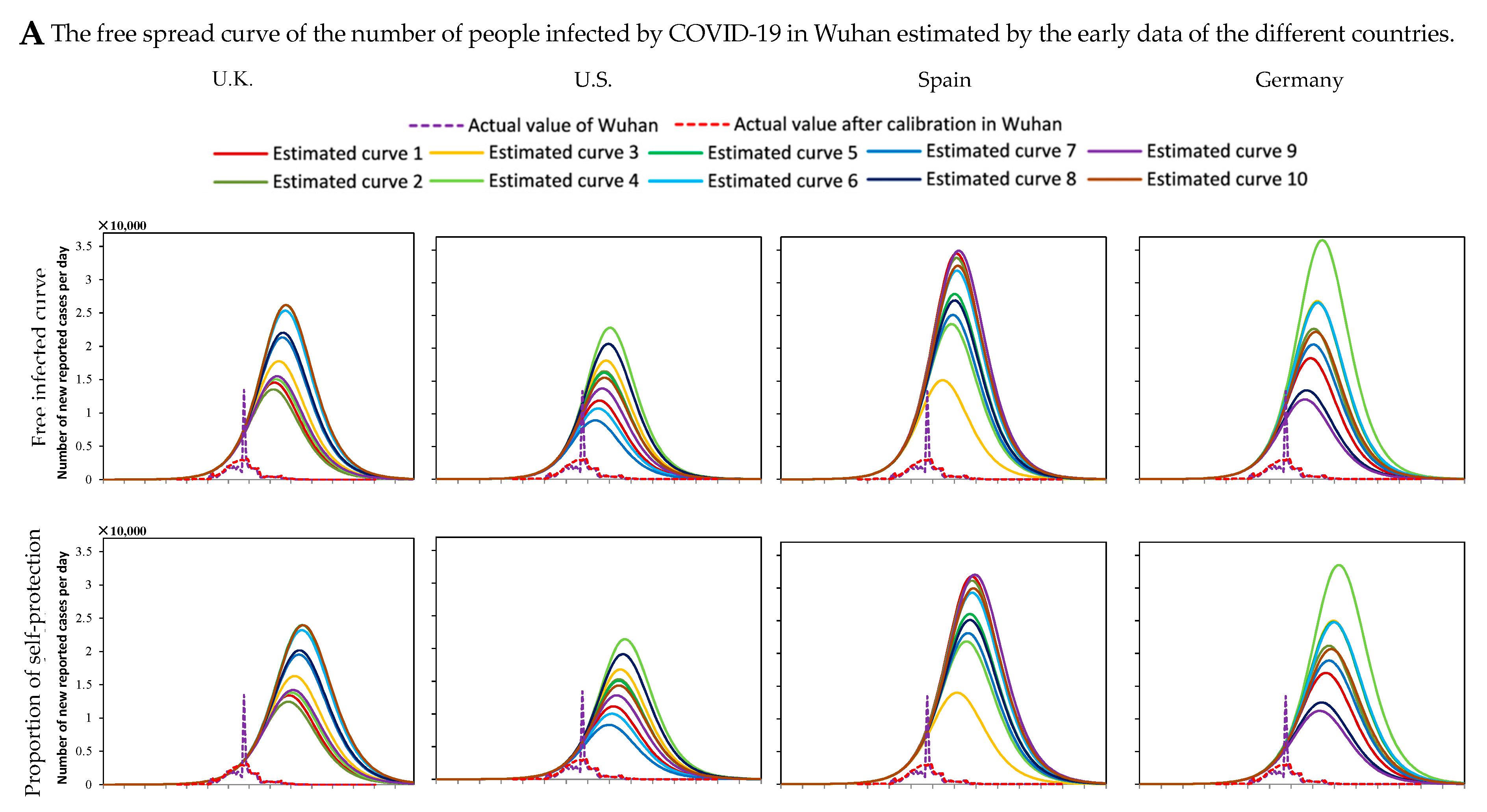
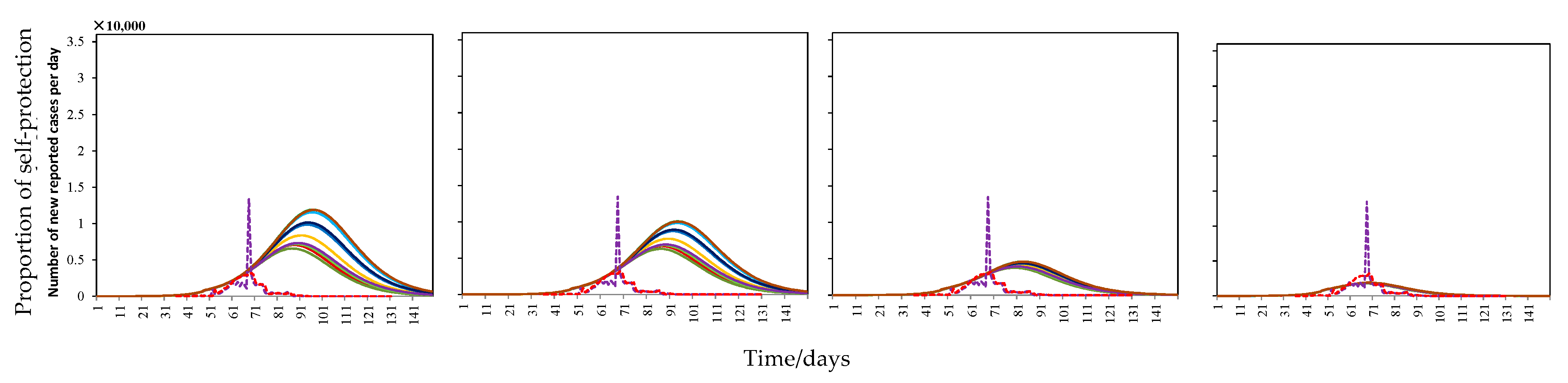
3.3. Experiment Analysis of the Influence of Different Self-Protection Measures to Mitigate the Spread of COVID-19

This section mainly discusses the influence of self-protection measures under different proportions of the effective self-protection of people and quarantines of different intensities to mitigate the spread of COVID-19. We used the intervention time of when a group of pneumonia cases with an unknown etiology were first published by Wuhan’s Municipal Health Commission as the baseline (11 January 2020, 35th day) and set the proportion of people using self-protection measures as 0.1, 0.2, 0.3, and 0.4 of the total number of humans (Figure 7A). Then, we adjusted the proportion of the population using self-protection measures ($\epsilon$) to 0.1, 0.2, 0.3, and 0.4 under grid sizes of 500, 250, 100, and 10 m, respectively (Figure 7B).

Figure 7A shows that the free infected curve of COVID-19 gradually moved further away from the actual infected curve of Wuhan as the proportion of people taking self-protection measures increased. The changing trend is mainly reflected in the delay time of a peak. However, the effect on reducing the peak value was mild. If we want to achieve an ideal result, the amount of needed self-protection resources is unimaginable. At the same time, self-protection measures do not fundamentally cut off the path of spread of the virus, but only reduces the probability of infection. Therefore, we suggest that the role of taking self-protection measure is mainly to delay the arrival of an epidemic peak and to strive for more time for the government to prepare.

Figure 7B shows that in the 500 and 250 m, self-protection measures have effects on reducing the size of the peak and delaying the time of the peak. However, the curve of people infected with COVID-19 hardly changed in the grid sizes of 100 and 10 m. This indicates that the effect of self-protection measures is not obvious under strict quarantine measures. This is mainly because the implementation of strict quarantine measures makes the area of movement of infected patients very small, and self-protection measures are difficult to implement effectively at this time. For example, when two people are isolated at home, it does not matter whether they wear face masks or not. Therefore, we suggest that, under strict quarantine measures, some types of resources of self-protection measures, such as face masks, medical clothes, hand sanitizer, and disinfectant, should be concentrated in the high-risk population who need to go out or come into contact with infected patients, such as medical staff, material distribution staff, and relevant leaders.

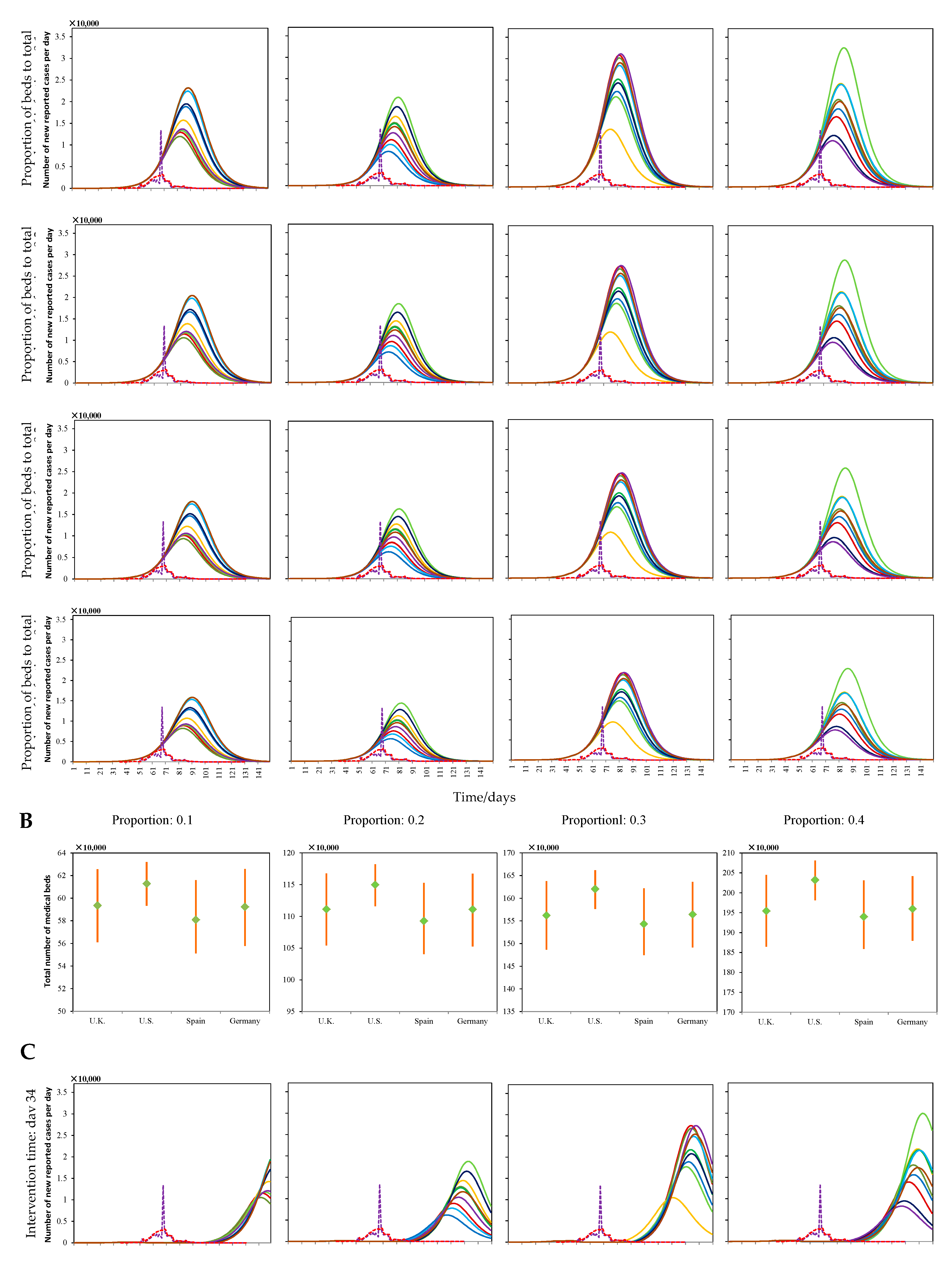
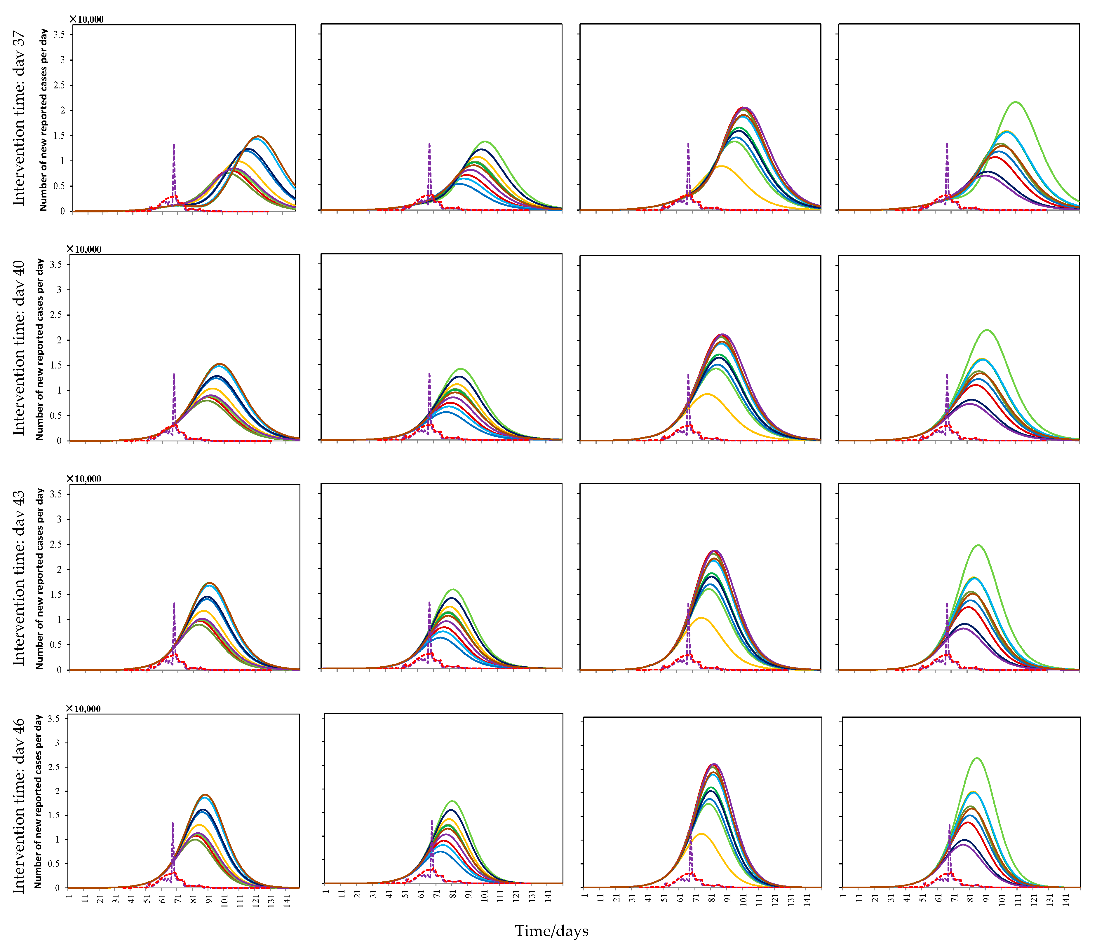
3.4. Experiment Analysis of the Influence of Different Hospital Isolation Measures to Mitigate the Spread of COVID-19

This section mainly discusses the influence of hospital isolation measures with different numbers of medical beds and different intervention times on mitigating the spread of COVID-19. The number of medical beds were calculated according to the percentage of people infected every day (including symptomatic and asymptomatic cases). We took the intervention time as when the first batch of hospitals was designated in Wuhan (20 January 2020, 44th day) and set the proportion of medical beds ($\delta$) to 0.1, 0.2, 0.3, and 0.4 (Figure 8A,B). Then, we fixed the ratio of the number of invested beds to 0.1 and adjusted the intervention time to the 34th, 37th, 40th, 43rd, and 46th days, respectively (Figure 8C).

Figure 8A shows that the free infected curve of the COVID-19 decreased at the peak with the increase in the number of beds (the proportion increased), which emphasizes the effectiveness of hospital isolation measures. However, the time of peak arrival and the duration of the epidemic did not seem to change. This is mainly because there were a large number of undetected or ineffectively quarantined cases in the crowds when the hospital isolation measures were put into use. Thus, the medical beds soon reached full capacity because of the limitation in the number of medical beds. Figure 8B shows that the total number of medical beds required was approximately 580,000 for the proportion of 0.1, which is difficult to achieve in reality.

Figure 8C shows that the free infected curve shifted to the left as the intervention time moved forward. The changing trend is mainly reflected in the increase in the time of peak arrival and the epidemic duration, but the peak did not seem to change. After maintaining a low level of epidemic spread for a short time, medical beds reached full capacity and the epidemic broke out again on a large scale. At this time, the medical system collapsed and the scale of the outbreak was similar to the original state of spread. The U.S. seems to be facing the same problem; therefore, we suggest that other effective measures must be adopted to reduce the pressure on the medical system.

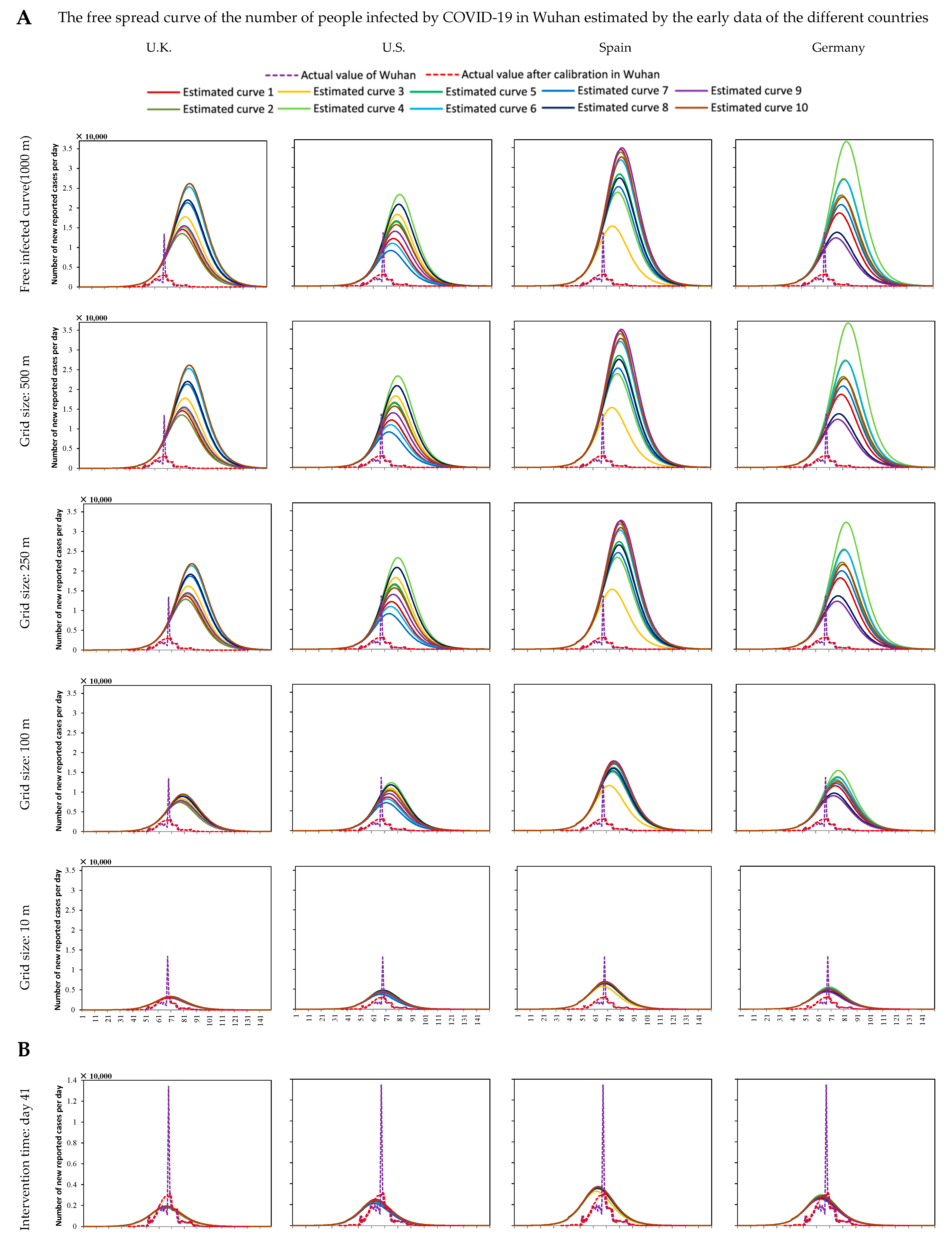
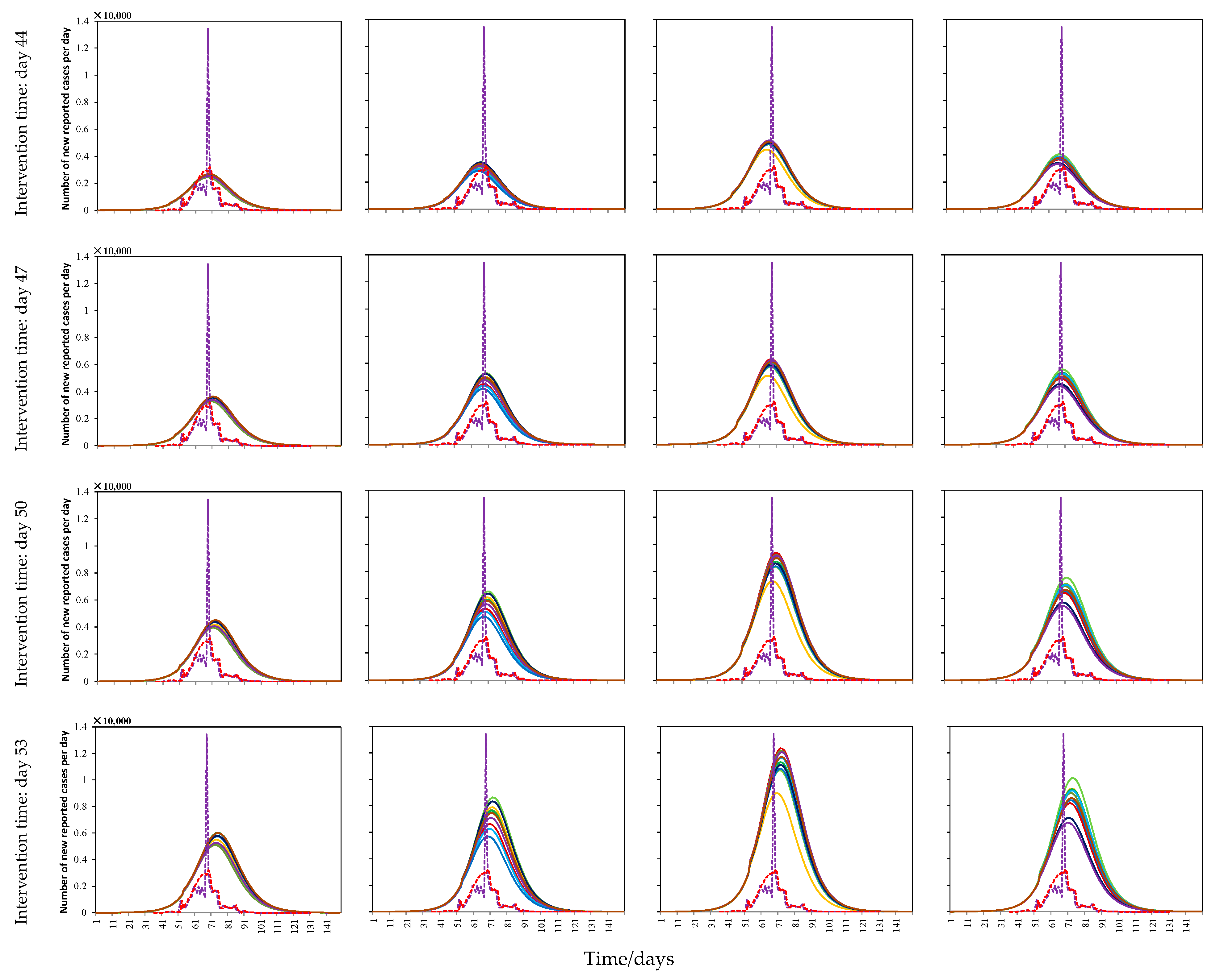
3.5. Model Validation under Actual Interventions of COVID-19 in Wuhan

In this section, the actual quarantine, the number of medical beds, and the proportion of people effectively wearing face masks (a self-protection measure) were used to verify the reliability of the model. In terms of quarantine measures, we used a 10 m grid to approximately represent the home quarantine measures implemented in Wuhan; the intervention time was 24 January 2020, when Wuhan implemented a “lockdown”. For hospital isolation measures, there were 68 designated hospitals in Wuhan, including 16 fangcang shelter hospitals and “huoshenshan” and “leishenshan” hospitals, with a total of 38,782 beds. Thus, the proportion of beds was approximately 0.06; the intervention time was the time when the first batch of designated hospitals were put into operation (20 January 2020). Due to the fact that the total number of humans complying with the self-protection measures was difficult to obtain, the proportion of people taking self-protection measures in Wuhan was represented by the proportion of those effectively wearing face masks. We assumed that each medical member of staff used two face masks every day and that every citizen used one face mask every three days. Thus, Wuhan needed to consume 2.1744 million face masks per day as the total number of medical staff in Wuhan was approximately 108,720 (including local and support medical staff), and the total population of Wuhan was approximately 14.18 million. According to the statistics, Wuhan received a total of 55.1 million face masks (including N95 and medical–surgical masks) during the period from 3 to 13 February 2020. Therefore, we set the daily effective proportion of wearing masks to 0.1; the intervention time of self-protection measure was the time when a group of pneumonia cases with an unknown etiology was first described by Wuhan’s Municipal Health Commission (11 January 2020). The results are shown in Figure 9.

Figure 9 shows that: the free infected curve continuously shrunk to the actual epidemic curve of Wuhan under the three interventions and the final result was fairly consistent with the actual curve of Wuhan. This also showed the effectiveness of the model used in this study. Among them, quarantine measures were the most effective, and hospital isolation and self-protection measures were mainly reflected in reducing the small peak of infection and delaying the spread of COVID-19 in the early stage (the curve moved to the left). However, there was some deviation between the final curve and the actual curve for Wuhan, which is mainly because of the following reasons:

• There was a certain difference between the free spread trend of COVID-19 estimated by the early data of other countries and the trend in Wuhan city itself;
• There were some errors in the case detection and data recording in Wuhan city because of the large amount of unknown information about the new virus in the early stage;
• There was still an obvious difference between the distribution of the population and the actual situation, such as there was no crowd activity around lakes, fields, and wasteland.

4. Discussion

Facing the increasingly serious threat of COVID-19, all countries urgently need to use computer modeling to determine the best strategy to mitigate the impact of COVID-19. The type of interventions, the intensity and scope of their implementation, and the intervention time differ in different countries because of the differences in the geographical environmental factors such as the development state of the epidemic, urban building distribution, peoples’ lifestyles, and economic development. At the same time, those are also the key to the effectiveness of COVID-19 prevention and control measures. We aimed to put forward a model that can integrate spatial and temporal information to further simulate the effectiveness of epidemic prevention and the control of non-pharmaceutical interventions under the influence of more complex natural and social factors, as well as to find better information about the spatiotemporal diffusion pattern of the COVID-19. Meanwhile, the practical significance of the model parameters can be mapped to the geographical space rather than only staying within the significance of mathematics, which can provide more direct instructive information for the implementation of specific invention policies.

This study has several limitations. Due to the fact that the existing data related to epidemic cases were not complete, there are still many uncertainties in the research on the mechanism of COVID-19 dynamic transmissions, such as the asymptomatic spread rate and the infectivity of the incubation period. Although model parameters have been referred to in research in famous international journals [1,16,55], a large number of unknown parameters were still ineluctably included in the dynamic model of COVID-19. It is worth noting that our focus was not on forecasting the epidemic situation; instead, the curve of the COVID-19 dynamics model were mainly used to evaluate and quantify the changes before and after the implementation of an intervention. Moreover, due to the lack of data on spatiotemporal attributes such as patients’ tracking data, residents’ activity data, passengers’ travel data of buses and subways, and mobile location data, we did not establish the relationship between the grid cells and the corresponding geographic attributes. However, those data are usually difficult to obtain in a public health safety emergency, which usually features missing or incomplete coverage.

In this study, the transmission model of COVID-19 was a generalized model of the macro-perspective. It is worth noting that we paid more attention to the realistic guiding significance of the prevention and control model under a discrete grid rather than the simulation for the fine-grained location of patients. The conclusion of the prevention and control model based on the generalized propagation model has positive significance. For example, in January 2021, the COVID-19 outbreaks occurred in Shanghai and Shijiazhuang, China [57,58]. Shijiazhuang carried out the detection for all the residents, while Shanghai only detected approximately 10,000 people who had close contact with each other. The authors believed that the main reason for this is that the patients in Shijiazhuang were in rural areas, so detailed tracking data could not be obtained. However, Shanghai is a developed city, so it was easier to obtain data for those in close contact with patients. These two methods are actually commonly used to search the potential patients—that is, a simple model based on generalization. The difference is that Shijiazhuang is a buffer based on points, while Shanghai is based on detailed patient tracking. At the same time, as diffusion models such as preferential diffusion or of advection type mainly use specific activity data to simulate the diffusion of people’s lives, the results of fine-grained spread model are more concentrated than the generalized model in the same infected degree. Therefore, the prevention and control model based on the discrete grid can achieve better results under the fine-grained propagation evolution. The more concentrated the infected areas, the more the uninfected areas are protected by quarantine and hospital isolation measures. Meanwhile, the authors indicated that even if the detailed epidemic data can be obtained, these only included the location where patients showed symptoms but the infected location is still not known; in other words, the current spread models of COVID-19 have the problem of scientific verification.

This study preliminarily and objectively described the spatiotemporal transmission law and development trend of COVID-19 under different interventions from the perspective of geography. It established the relationship between the model parameters and the actual geographical significance. We aimed to the positive significance of the prevention and control model under the discrete grid to the reality. In future work, we hope to solve the problem of the scientific verification of an intervention model through multi-source data, such as network news data, global event databases, and remote sensing data. Our spatiotemporal transmission model of COVID-19 can be improved with more multi-source data, describing the crowd aggregation and interaction, to further guide the diffusion track and allocation of infected humans. This could improve the authenticity of the model. The model also provides a possible way to analyze the problems of medical resource allocation, spatial location selection, and the plan of receiving infected patients. Finally, mapping between socioeconomic data and grid areas can be established to quantify the cost to the economy and of resources under different interventions, providing better guidance for scientific decision making and accurate implementation for prevention and control. To sum up, these will be the focus and problem of our subsequent research.

5. Conclusions

In summary, this study combined a COVID-19 dynamics spread model with geography from a new perspective to quantitatively analyze the impact of interventions. The model can provide more direct and effective information for the formulation of prevention and control policies, which has important practical significance. A discrete grid was used to divide the geographical regions and the spatiotemporal spread model of COVID-19 was designed based on the features of residents’ daily activities. Meanwhile, the granularity and virtual real line of the boundary of the discrete grid was introduced to describe the intensity of the physical quarantine measures implemented and the connectivity of adjacent spaces separately. Hospital isolation and self-protection measures were integrated into the model, and parameters were mapped to the corresponding grid regions based on the spatial correlations. Finally, the COVID-19 dynamics model was used for the quantitative analysis of the number of humans infected under different interventions. Through the simulation of experiments, the conclusions were as follows:

• Quarantine measures were the most effective for prevention and control, especially for infectious diseases with a high infectivity. They were shown to be able to drastically reduce the number of infected humans, advance the arrival of the maximum number of infected humans, and shorten the duration of the COVID-19 outbreak. However, quarantine measures are only effective under a sufficient implementation intensity, and the effect of quarantine measures decreases with the delay of the intervention time. Moreover, strict quarantine measures may be ignored in the early stages of an outbreak because the spread of the epidemic is mild during this period.
• Hospital isolation measures mainly played a role in the early stage of the COVID-19 outbreak. The increase in medical beds effectively reduced the number of infected humans, but had only a small effect on the arrival time of maximum number of infected humans and the duration of the COVID-19 outbreak. Moreover, using an earlier intervention time could effectively delay the arrival of the maximum number of infected humans, but an outbreak would still occur again when the medical beds reach capacity, with a scale similar to that of original infectious state.
• Self-protection measures were able to reduce the number of infected humans and to largely delay the arrival of the peak number of infected humans, providing the government with more time to prepare. However, self-protection measures almost had no effect under stricter quarantine measures. Therefore, medical resources should be concentrated in hospitals and other places in urgent need under the conditions of strict quarantine measures.
• This study qualitatively and quantitatively analyzed the impact of quarantine, self-protection, and hospital isolation measures to slow the spread of COVID-19, which was scientific and reasonable. Meanwhile, the result possess a high interpretability for the practical significance of intervention, and the model parameters can map the model to the actual geographical area, which is helpful for the scientific formulation of specific epidemic prevention and control decisions.

References

1. Chen, N.; Zhou, M.; Dong, X.; Qu, J.; Gong, F.Y.; Han, Y.; Qiu, Y.; Wang, J.L.; Liu, Y.; Wei, Y.; et al. Epidemiological and clinical characteristics of 99 cases of 2019 novel coronavirus pneumonia in Wuhan, China: A descriptive study. Lancet 2020, 395, 507–513. [Google Scholar] [CrossRef] [Green Version]
2. Li, Q.; Guan, X.H.; Wang, X.Y.; Wu, P.; Wang, X.Y.; Zhou, L.; Tong, Y.Q.; Ren, R.Q.; Leung, K.S.M. Early spread dynamics in Wuhan, China, of novel coronavirus-infected pneumonia. Natl. Engl. J. Med. 2020, 382, 1199–1207. [Google Scholar] [CrossRef]
3. Tian, H.Y.; Liu, Y.H.; Li, Y.D.; Wu, C.H.; Chen, B.; Kraemer, M.U.G.; Li, B.Y.; Cai, J.; Yang, Q.Q.; Cui, Y.J. An investigation of spread control measures during the first 50 days of the COVID-19 epidemic in China. Science 2020, 6491, 638–642. [Google Scholar] [CrossRef] [PubMed] [Green Version]
4. Chan, J.; Yuan, S.F.; Kok, K.; To, K.K.W.; Chu, H.; Yang, J.; Xing, F.F.; Liu, J.L.; Yip, C.C.Y.; Poon, R.W.S. A family cluster of pneumonia associated with the 2019 novel coronavirus indicating person-to-person spread: A study of a family cluster. Lancet 2020, 395, 514–523. [Google Scholar] [CrossRef] [Green Version]
5. Currie, C.S.M.; Fowler, J.W.; Kotiadis, K.; Monks, T.; Onggo, B.S.; Roberston, D.A.; Tako, A.A. How simulation modeling can help reduce the impact of COVID-19. J. Simul. 2020, 2, 83–97. [Google Scholar] [CrossRef] [Green Version]
6. Wu, J.T.; Leung, K.; Leung, G.M. Nowcasting and forecasting the potential domestic and international spread of the 2019-nCoV outbreak originating in Wuhan, China: A modelling study. Lancet 2020, 10225, 689–697. [Google Scholar] [CrossRef] [Green Version]
7. Wang, H.W.; Wang, Z.Z.; Dong, Y.Q.; Chang, R.J.; Xu, C.; Yu, X.Y.; Zhang, S.X.; Tsamlag, L.; Shang, M.L.; Wang, Y. Phase-adjusted estimation of the number of Coronavirus Diseases 2019 cases in Wuhan, China. Cell Discov. 2020, 6, 10. [Google Scholar] [CrossRef] [PubMed] [Green Version]
8. Zhao, S.; Lin, Q.Y.; Ran, J.J.; Musa, S.S.; Yang, G.P.; Wang, W.M.; Lou, Y.J.; Gao, D.Z.; Yang, L.; He, D.H. Preliminary estimation of the basic reproduction number of novel coronavirus (2019-nCoV) in China, fro-m 2019 to 2020: A data-driven analysis in the early phase of the outbreak. Int. J. Infect. Dis. 2020, 92, 214–217. [Google Scholar] [CrossRef] [PubMed] [Green Version]
9. Zhou, T.; Liu, Q.; Yang, Z.; Liao, J.Y.; Yang, K.X.; Bai, W.; Lü, X.; Zhang, W. Preliminary prediction of the basic reproduction number of the Wuhan novel coronavirus 2019-nCoV. J. Evid. Based Med. 2020, 13, 3–7. [Google Scholar] [CrossRef] [PubMed]
10. Read, J.M.; Bridgen, J.R.E.; Cummings, D.A.T.; Ho, A.; Jewell, C.P. Novel coronavirus 2019-nCoV: Early estimation of epidemiological parameters and epidemic size estimates. Phil. Trans. R. Soc. B 2020, 376, 20200265. [Google Scholar] [CrossRef]
11. Jumpen, W.; Wiwatanapataphee, B.; Wu, Y.H.; Tang, I.M. A SEIQR model for pandemic influenza and its parameter identification. Int. J. Pure Appl. Math. 2020, 52, 247–265. Available online: http://ijpam.eu/contents/2009-52-2/8/index.html (accessed on 10 January 2020).
12. Maier, B.F.; Brockmann, D. Effective containment explains sub-exponential growth in confirmed cases of recent COVID-19 outbreak in Mainland China. Science 2020, 368, 742–746. [Google Scholar] [CrossRef] [Green Version]
13. Crokidakis, N. COVID-19 spreading in Rio de Janeiro, Brazil: Do the policies of social isolate-on really work? Chaos Solitons Fractals 2020, 136, 109930. [Google Scholar] [CrossRef]
14. Viguerie, A.; Lorenzo, G.; Auricchio, F.; Baroli, D.; Hughes, T.J.R.; Patton, A.; Reali, A.; Yankeelov, T.E.; Veneziani, A. Simulating the spread of COVID-19 via a spatially-resolved susceptible–exposed–infected–recovered–deceased (SEIRD) model with heterogeneous diffusion. Appl. Math. Lett. 2020, 111, 106617. [Google Scholar] [CrossRef] [PubMed]
15. Cooke, K.L.; Driessche, P.V.D. Analysis of an SEIRS epidemic model with two delays. J. Math. Biol. 1996, 35, 240–260. [Google Scholar] [CrossRef]
16. Okuonghae, D.; Omame, A. Analysis of a mathematical model COVID-19 crowds dynamics in Lagos, Nigeria. Chaos Solitons Fractals 2020, 139, 110032. [Google Scholar] [CrossRef] [PubMed]
17. Davies, N.G.; Klepac, P.; Liu, Y.; Perm, K.; Jit, M.; Eggo, R.M. Age-dependent effects in the spread and control of COVID-19 epidemics. Nat. Med. 2020, 26, 1205–1211. [Google Scholar] [CrossRef] [PubMed]
18. Davies, N.G.; Kucharski, A.J.; Eggo, R.M.; Gimma, A.; Edmunds, W.J. Effects of non-pharmaceutical interventions on COVID-19 cases, deaths, and demand for hospital services in the UK: A modelling study. Lancet 2020, 7, e375–e385. [Google Scholar] [CrossRef]
19. Kassa, S.M.; Njagarah, J.B.H.; Terefe, Y.A. Analysis of the mitigation strategies for COVID-19: From mathematical modelling perspective. Chaos Solitons Fractals 2020, 138, 109968. [Google Scholar] [CrossRef]
20. Stadnytskyi, V.; Bax, C.E.; Bax, A.; Anfinrud, P. The airborne lifetime of small speech droplets and their potential importance in SARS-CoV-2 spread. Proc. Natl. Acad. Sci. USA 2020, 117, 11875–11877. [Google Scholar] [CrossRef]
21. Ribeiro, M.H.D.M.; Silva, R.G.D.; Mariani, V.C.; Coelho, L.D.S. Short-term forecasting COVID-19 cumulative confirmed cases: Perspectives for Brazil. Chaos Solitons Fractals 2020, 135, 109853. [Google Scholar] [CrossRef]
22. Chakraborty, T.; Ghosh, I. Real-time forecasts and risk assessment of novel coronavirus (COVID-19) cases: A data-driven analysis. Chaos Solitons Fractals 2020, 135, 109850. [Google Scholar] [CrossRef] [PubMed]
23. Li, S.J.; Song, K.; Yang, B.R.; Gao, Y.C.; Gao, X.F. Preliminary assessment of the COVID-19 outbreak using 3-staged model e-ISHR. J. Shanghai Jiaotong Univ. Sci. 2020, 25, 157–164. [Google Scholar] [CrossRef] [Green Version]
24. Zhang, L.Y.; Li, D.C.; Ren, J.L. Analysis of COVID-19 by Discrete Multi-stage Dynamics System with Time Delay. Geomat. Inf. Sci. Wuhan Univ. 2020, 45, 658–666. [Google Scholar] [CrossRef]
25. Lymperopoulos, I.N. #stayhome to contain COVID-19: Neuro-SIR-Neurodynamical epidemic modeling of infection patterns in social networks. Expert Syst. Appl. 2021, 165, 113970. [Google Scholar] [CrossRef] [PubMed]
26. Bouchnita, A.; Jebrane, A. A hybrid multi-scale model of COVID-19 spread dynamics to assess the potential of non-pharmaceutical interventions. Chaos Solitons Fractals 2020, 138, 109941. [Google Scholar] [CrossRef]
27. Lin, Q.Y.; Zhao, S.; Gao, D.Z.; Lou, Y.J.; Yang, S.; Musa, S.; Wang, M.H.; Cai, Y.L.; Wang, W.M.; Yang, L. A conceptual model for the coronavirus disease 2019 (COVID-19) outbreak in Wuhan, China with individual reaction and governmental action. Int. J. Infect. Dis. 2020, 93, 211–216. [Google Scholar] [CrossRef]
28. Fang, Y.Q.; Nie, Y.T.; Penny, M. Spread dynamics of the COVID-19 outbreak and effectiveness of government interventions: A data-driven analysis. J. Med. Virol. 2020, 92, 645–659. [Google Scholar] [CrossRef] [PubMed] [Green Version]
29. Tang, B.; Wang, X.; Li, Q.; Bragazzi, N.L.; Tang, S.Y.; Xiao, Y.N.; Wu, J.H. Estimation of the spread risk of the 2019-nCoV and its impaction for public health interventions. J. Clin. Med. 2020, 9, 462. [Google Scholar] [CrossRef] [Green Version]
30. Chu, D.K.; Duda, S.; Solo, K.; Yaacoub, S.; Schunemann, H. Physical distancing, Face masks, and eye protection to prevent person-to-person spread of SARS-CoV-2 and COVID-19: A systematic review and meta-analysis. Lancet 2020, 72, 1500. [Google Scholar] [CrossRef]
31. Ma, Z.H.; Wang, S.F.; Li, X.H. A generalized infectious model induced by the contacting distance (CTD). Nonlinear Anal. Real World Appl. 2020, 54, 103113. [Google Scholar] [CrossRef]
32. Gostic, K.; Gomez, A.C.R.; Mummah, R.O.; Kucharski, A.J.; Lloyd-Smith, J.O. Estimated effectiveness of symptom and risk screening to prevent the spread of COVID-19. eLife 2020, 9, e55570. [Google Scholar] [CrossRef]
33. Wells CRSah, P.; Moghadas, S.M.; Pandey, A.; Shoukat, A.; Wang, Y.N.; Wang, Z.; Meyers, L.A.; Singer, B.H.; Galvani, A.P. Impact of international travel and border control measures on the global spread of the novel 2019 coronavirus outbreak. Proc. Natl. Acad. Sci. USA 2020, 117, 7504–7509. [Google Scholar] [CrossRef] [Green Version]
34. Hellewell, J.H.; Abbott, S.; Gimma, A.; Bosse, N.I.; Jarvis, C.I.; Russell, T.; Munday, J.D.; Kucharski, A.J.; Edmunds, W.J. Feasibility of controlling COVID-19 outbreaks by isolation of cases and contacts. Glob. Health 2020, 4, e488–e496. [Google Scholar] [CrossRef] [Green Version]
35. Wölfel, R.; Corman, V.M.; Gugemos, W.; Seilmaier, M.; Zange, S.; Müller, M.A.; Niemeyer, D.N.; Jones, T.C.; Vollmar, P.; Hoelscher, M. Virological assessment of hospitalized patients with COVID-2019. Nature 2020, 281, 465–469. [Google Scholar] [CrossRef] [Green Version]
36. Rosa, G.L.; Bonadonna, L.; Luca, L.; Kenmoe, S.; Suffredini, E. Coronavirus in water environments: Occurrence, persistence and concentration methods—A scoping review. Water Res. 2020, 179, 115899. [Google Scholar] [CrossRef]
37. Leclerc, Q.J.; Fuller, N.M.; Knight, L.E.; Knight, G.M. What settings have been linked to SARS-CoV-2spread cluster? [version 1; peer review:1 approved with reservations]. Wellcome Open Res. 2020, 5, 83. [Google Scholar] [CrossRef]
38. Lu, J.Y.; Gu, J.N.; Xu, C.H.; Su, W.Z.; Lai, Z.S.; Zhou, D.Q.; Yu, C.; Xu, B.; Yang, Z.C. COVID-19 outbreak associated with Air conditioning in restaurant, Guangzhou, China, 2020. Emerg. Infect. Dis. 2020, 26, 1628–1631. [Google Scholar] [CrossRef] [PubMed]
39. Morawska, L.; Cao, J.J. Airborne spread of SARS-CoV-2: The world should face the reality. Environ. Int. 2020, 139, 105730. [Google Scholar] [CrossRef] [PubMed]
40. Dehning, J.; Zierenberg, J.; Spitzner, F.P.; Wibral, M.; Neto, J.P.; Wilczek, M.; Priesemann, W. Inferring change point in the spread of COVID-19 reveals the effectiveness of interventions. Science 2020, 6500, eabb9789. [Google Scholar] [CrossRef]
41. Thu, T.P.B.; Ngoc, P.N.H.; Hai, N.M.; Tuan, L.A. Effect of the social distancing measures on the spread of COVID-19 in 10 highly infected countries. Sci. Total. Environ. 2020, 742, 140430. [Google Scholar] [CrossRef] [PubMed]
42. Barmparis, G.D.; Tsironis, G.P. Estimating the infection horizon of COVID-19 in eight counties with a data-driven approach. Chaos Solitons Fractals 2020, 135, 109842. [Google Scholar] [CrossRef]
43. Han, W.G. Data-driven and model-driven spatiotemporal data ming-respective case study in traffic flow data and epidemic data. Chin. Acad. Sci. 2006. Available online: http://ir.igsnrr.ac.cn/handle/311030/106 (accessed on 12 January 2020).
44. Franch-Pardo, I.; Napoletano, B.M.; Rosete-Verges, F.; Billa, L. Spatial analysis and GIS in the study of COVID-19. A Review. Sci. Total. Environ. 2020, 739, 140033. [Google Scholar] [CrossRef]
45. Feng, M.X.; Fang, Z.X.; Lu, X.B.; Xie, Z.F.; Xiong, S.W.; Zheng, M.; Huang, S.Q. Traffic Analysis Zone-Based Epidemic Estimation Approach of COVID-19 Based on Mobile Phone Data: An Example of Wuhan. Geomat. Inf. Sci. Wuhan Univ. 2020, 45, 651–657, 681. [Google Scholar] [CrossRef]
46. Sugg, M.M.; Spaulding, R.J.; Lane, S.J.; Runkle, J.D.; Harden, S.R.; Hege, A.; Lyer, L.S. Mapping community-level determinants of COVID-19 spread in nursing homes: A multi-scale approach. Sci. Total. Environ. 2020, 752, 141946. [Google Scholar] [CrossRef] [PubMed]
47. Ren, H.Y.; Zhao, L.; Zhang, A.; Song, L.Y.; Liao, Y.L.; Lu, W.L.; Cui, C. Early forecasting of the potential risk zones of COVID-19 in China’s megacities. Sci. Total. Environ. 2020, 729, 138995. [Google Scholar] [CrossRef] [PubMed]
48. Fang, Z.X. Thinking and challenges of crow dynamics observation from the perspectives of public health and public security. Geomat. Inf. Sci. Wuhan Univ. 2020, 45, 1847–1856. [Google Scholar] [CrossRef]
49. Zwęgliński, T.; Radkowski, R. Fire and Rescue Units During COVID-19 Epidemic. Operational Functioning and Tasks in the First Months of SARS-CoV-2 activity. Zesz. Nauk. SGSP 2020, 76, 93–114. [Google Scholar] [CrossRef]
50. Cao, Z.D. Mathematical modeling and spatial analysis of spatiotemporal data-case study based on SARS epidemic in Guangzhou. Chin. Acad. Sci. 2008. Available online: http://ir.igsnrr.ac.cn/handle/311030/1774 (accessed on 12 January 2020).
51. Dong, E.; Du, H.; Gardner, L. An interactive web-based dashboard to track COVID-19 in real time. Lancet Infect. Dis. 2020, 20, 422–534. [Google Scholar] [CrossRef]
52. Cui, H.J.; Hu, T. Nonlinear regression in COVID-19 forecasting (in Chinese). Sci. Sin. Math. 2020, 50, 1–12. Available online: https://engine.scichina.com/doi/10.1360/SSM-2020-0055 (accessed on 12 January 2020).
53. Xia, J.Z.; Zhou, Y.; Li, Z.; Li, F.; Yue, Y.; Cheng, T.; Li, Q.Q. COVID-19 risk assessment driven by urban spatiotemporal big data: Case study of Guangdong-Hong Kong-Macao Greater Bay Area. Acta Geod. Et Cartogr. Sin. 2020, 49, 671–680. Available online: http://xb.sinomaps.com/CN/10.11947/j.AGCS.2020.20200080 (accessed on 12 January 2020).
54. Cauchemez, S.; Fraser, C.; Wan, M.D.; Donnelly, C.A.; Riley, S.; Rambaut, A.; Enouf, V.; Werf, S.V.D.; Ferguson, N.M. Middle east respiratory syndrome coronavirus: Quantification of the extent of the epidemic, surveillance biases, and transmissibility. Lancet Infect. Dis. 2020, 1, 50–56. [Google Scholar] [CrossRef] [Green Version]
55. Alberti, T.; Faranda, D. On the uncertainty of real-time predictions of epidemic growths: A COVID-19 case study for China and Italy. Commun. Nonlinear Sci. Numer. Simul. 2020, 90, 105372. [Google Scholar] [CrossRef] [PubMed]
56. Guo, L.; Yang, W.Q.; Bi, Y.F. Research on the Scale of Daily Life Unit Based on Residents’ Travel Characteristics. China Acad. J. Electron. Publ. House 2016, 1004–1015. Available online: https://kns.cnki.net/KCMS/detail/detail.aspx?dbcode=CPFD&filename=CSJT201604001098 (accessed on 12 January 2020).
57. Wang, C.; Zhu, R.X.; Wu, Y.T. Shanghai 168 Hours: How to Control the Epidemic in a Super City within A Week [EB/OL]. 2021. Available online: https://xw.qq.com/cmsid/20210202A019Z7/20210202A019Z700?ADTAG=hwb&pgv_ref=hwb&appid=hwbrowser&ctype=news (accessed on 11 July 2021).
58. Wei, Z. More than 20000 People in Shijiazhuang Have Been Transferred Urgently! This Epidemic Is Not as Simple as You Think [EB/OL]. 2021. Available online: https://new.qq.com/omn/20210113/20210113A02KCY00.html (accessed on 11 July 2021).
Figure 1. A diagram of the grid filling of traditional prevention and control units.
Ijgi 10 00480 g001
Figure 2. Schematic diagram of the model of quarantine measures based on a discrete grid.
Ijgi 10 00480 g002
Figure 3. Spatiotemporal spread model for infectious diseases based on a discrete grid.
Ijgi 10 00480 g003
Figure 4. Schematic diagram of hospital isolation measures (A) and self-protection measures (B).
Ijgi 10 00480 g004
Figure 5. The number of newly reported cases per day without any interventions. These should be listed as: (a) early U.K. data to simulate the free spread of COVID-19; (b) early U.S. data to simulate the free spread of COVID-19; (c) early Spanish data to simulate the free spread of COVID-19; (d) early German data to simulate the free spread of COVID-19. Small chart section: The red histogram represents the number of new early cases daily in each country, and the curve is the number of daily new cases without any interventions. Big graph section: The different colored solid-line curve represents the number of daily new cases in Wuhan without any interventions under the different parameters. The red dotted-line curve shows the actual number of newly reported cases in Wuhan after calibration, and the purple dotted-line curve represents the actual number of newly reported cases in Wuhan. Here, the starting time of the X coordinate in Wuhan is 28 December 2019 [9].
Ijgi 10 00480 g005
Figure 6. The change curve of newly reported cases per day in Wuhan under different quarantine measures. (Group (A) showed the change of infected curve under different grid sizes; Group (B) was the change of infected curve under different intervention times).
Ijgi 10 00480 g006aIjgi 10 00480 g006b
Figure 7. The change curve of the newly reported cases per day in Wuhan under different self-protection measures. (Group (A) was the change of infected curve under different proportion of people who complied with self-protection measures; Group (B) was the change of infected curve under different grid size and proportion of people who complied with self-protection measures).
Ijgi 10 00480 g007aIjgi 10 00480 g007bIjgi 10 00480 g007c
Figure 8. The change curve of newly reported cases per day in Wuhan under the different hospital isolation measures (Group (A) was the change of infected curve under different bed proportion; Group (B) was the number of beds needed under different bed proportions, and the length of the yellow vertical line and the green prism points indicates the 95% confidence interval and the median values of the total number of invested beds corresponding to 10 curves, respectively; Group (C) was the change of infection curve under different intervention time.).
Ijgi 10 00480 g008aIjgi 10 00480 g008bIjgi 10 00480 g008c
Figure 9. The change curve of newly reported cases per day in Wuhan under actual interventions.
Ijgi 10 00480 g009aIjgi 10 00480 g009b